A Study of the Spatial Difference of the Soil Quality of The Mun River Basin during the Rainy Season

 ,
, 
Abstract
1. Introduction
2. Data Collection
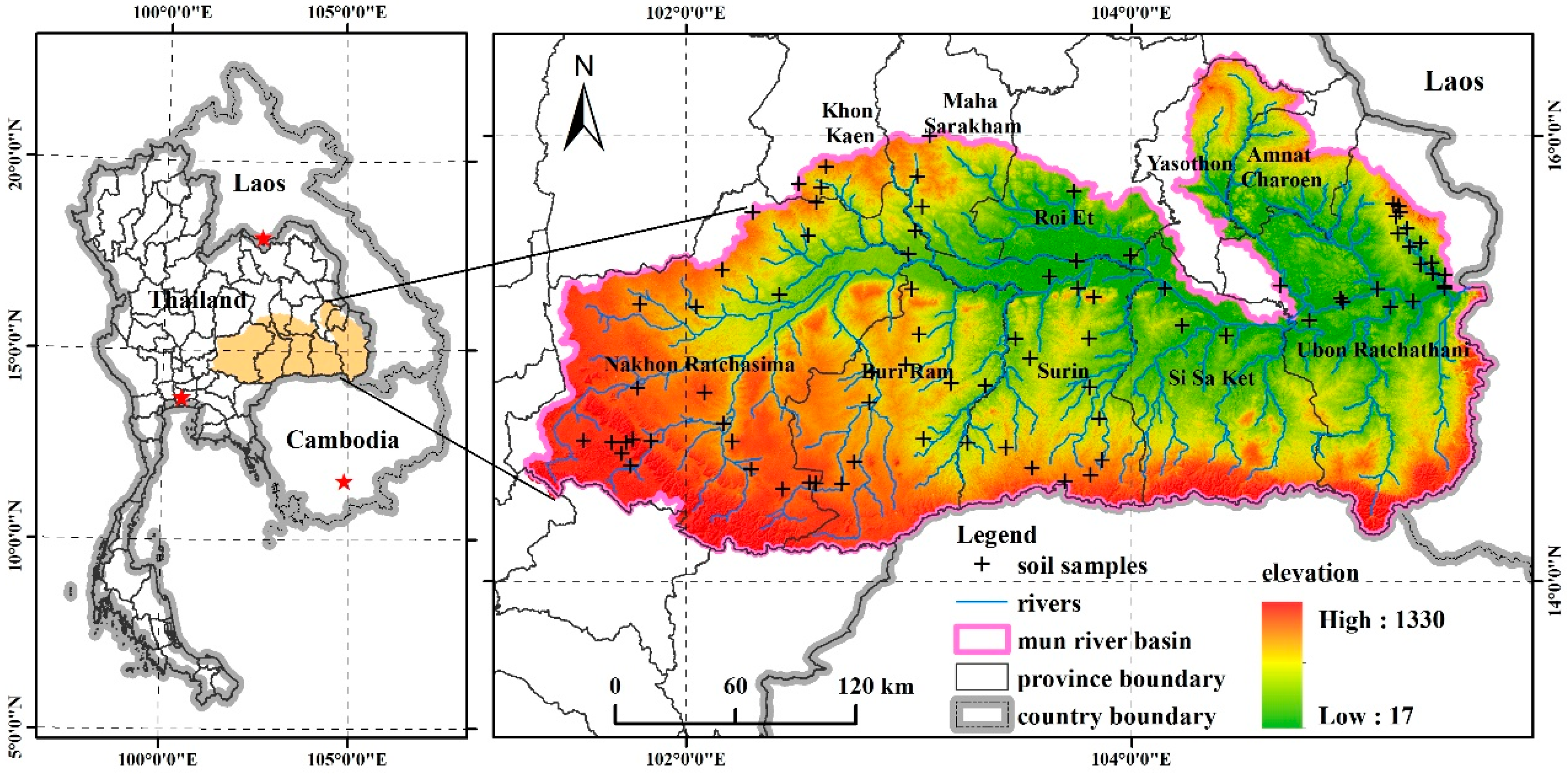
2.1. Study Area
2.2. Soil Sampling and Analysis
2.3. Auxiliary Data
3. Methods
3.1. Geographically Weighted Regression
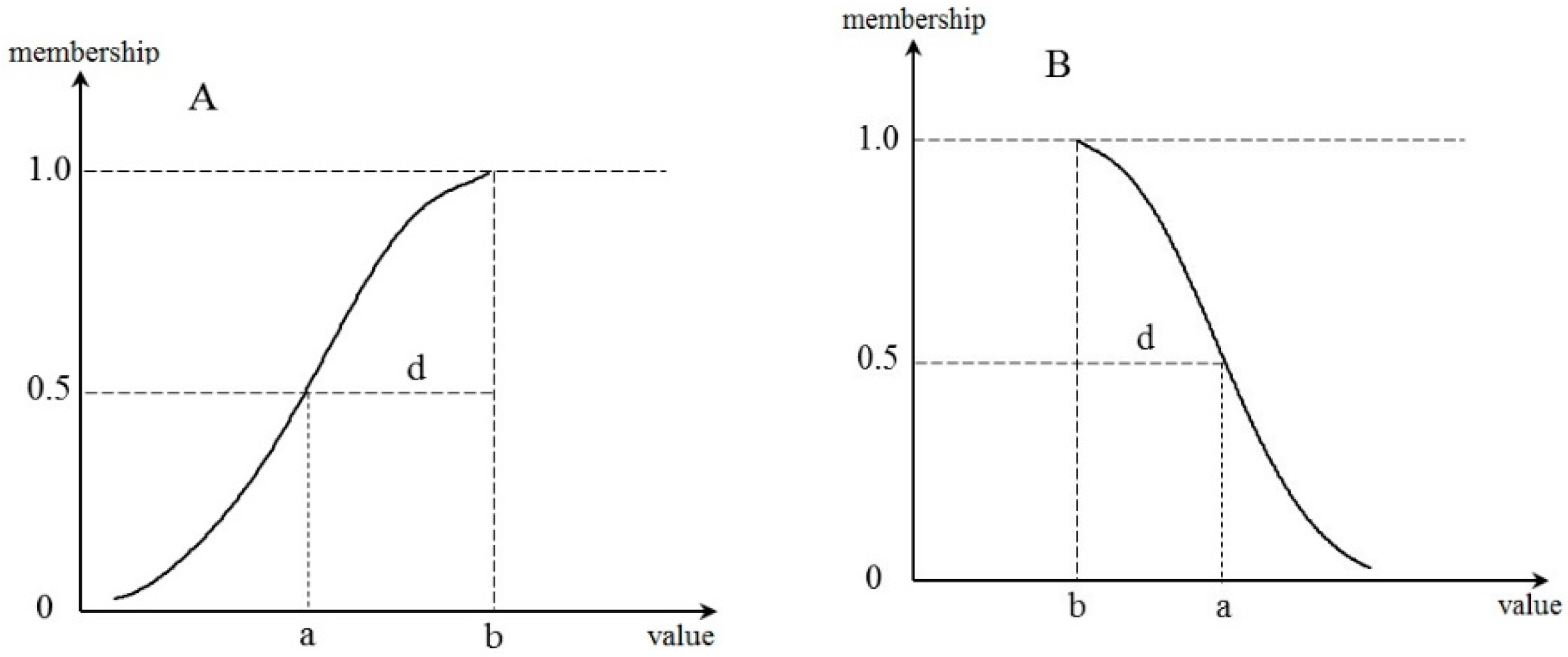
3.2. Fuzzy Logic Model
4. Results
4.1. Descriptive Statistics
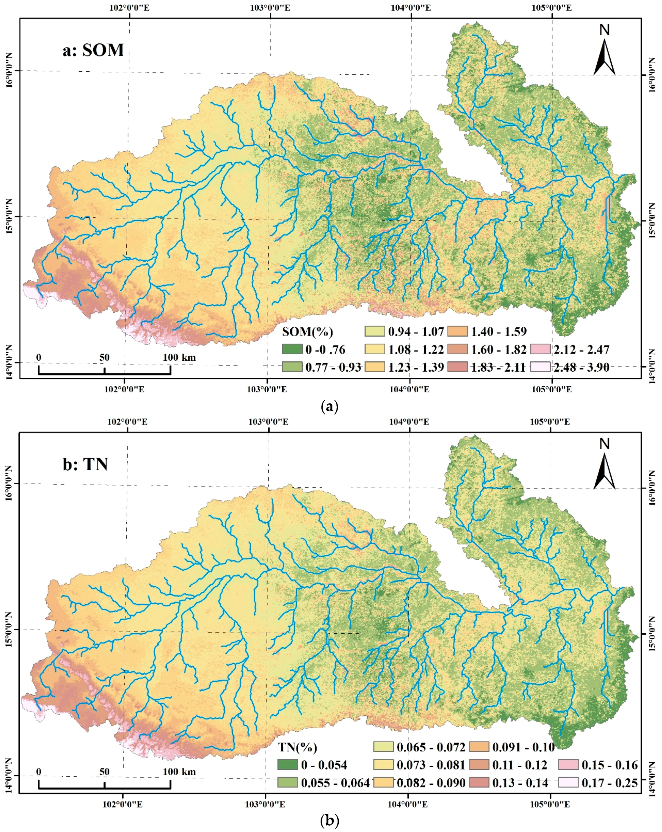
4.2. Soil Indicator Interpolation
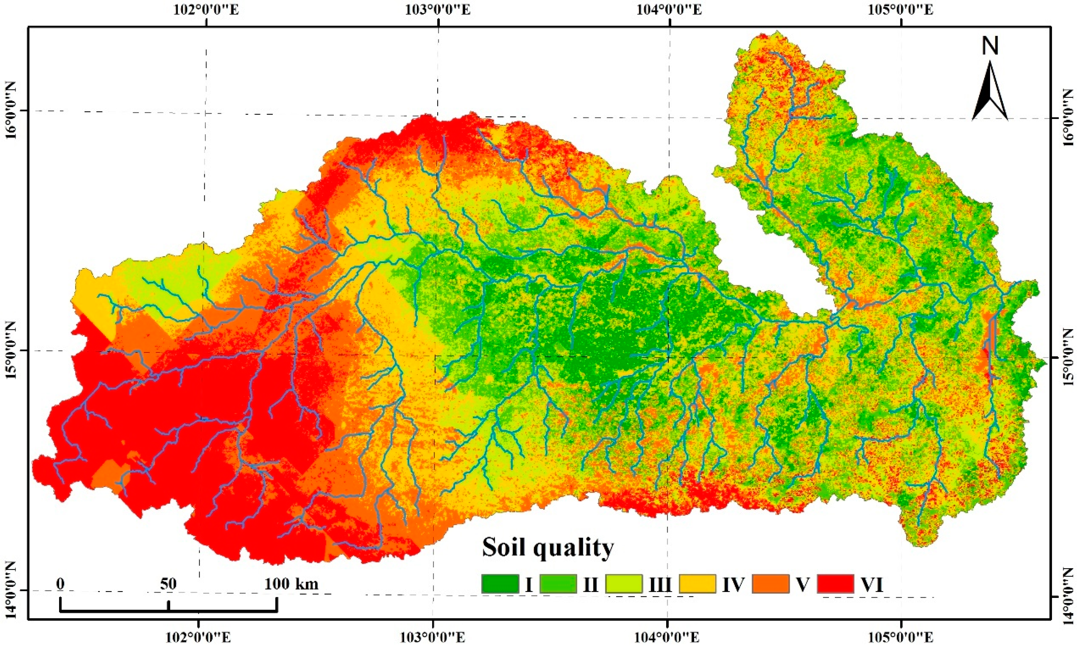
4.3. Soil Quality Assessment and Analysis
5. Discussion
6. Conclusions
Author Contributions
Funding
Conflicts of Interest
References
- Gavrilenko, E.G.; Ananyeva, N.D.; Makarov, O.A. Assessment of soil quality in different ecosystems (with soils of Podolsk and Serpukhov districts of Moscow oblast as examples). Eurasian Soil Sci. 2013, 46, 1241–1252. [Google Scholar] [CrossRef]
- Nabiollahi, K.; Golmohamadi, F.; Taghizadeh-Mehrjardi, R.; Kerry, R.; Davari, M. Assessing the effects of slope gradient and land use change on soil quality degradation through digital mapping of soil quality indices and soil loss rate. Geoderma 2018, 318, 16–28. [Google Scholar] [CrossRef]
- Doran, J.W.; Parkin, T.B. Defining and Assessing Soil Quality. In Defining Soil Quality for a Sustainable Environment; Special Publication, Soil Science Society of America: Madison, WI, USA, 1994; pp. 3–21. [Google Scholar]
- Zuber, S.M.; Behnke, G.D.; Nafziger, E.D.; Villamil, M.B. Multivariate assessment of soil quality indicators for crop rotation and tillage in Illinois. Soil Tillage Res. 2017, 174, 147–155. [Google Scholar] [CrossRef]
- Guo, L.; Sun, Z.; Ouyang, Z.; Han, D.; Li, F. A comparison of soil quality evaluation methods for Fluvisol along the lower Yellow River. Catena 2017, 152, 135–143. [Google Scholar] [CrossRef]
- Volchko, Y.; Norrman, J.; Rosen, L.; Norberg, T. A minimum data set for evaluating the ecological soil functions in remediation projects. J. Soils Sediments 2014, 14, 1850–1860. [Google Scholar] [CrossRef]
- Biswas, S.; Hazra, G.C.; Purakayastha, T.J.; Saha, N.; Mitran, T.; Roy, S.S.; Basak, N.; Mandal, B. Establishment of critical limits of indicators and indices of soil quality in rice-rice cropping systems under different soil orders. Geoderma 2017, 292, 34–48. [Google Scholar] [CrossRef]
- Cheng, J.; Ding, C.; Li, X.; Zhang, T.; Wang, X. Soil quality evaluation for navel orange production systems in central subtropical China. Soil Tillage Res. 2016, 155, 225–232. [Google Scholar] [CrossRef]
- Van Hall, R.L.; Cammeraat, L.H.; Keesstra, S.D.; Zorn, M. Impact of secondary vegetation succession on soil quality in a humid Mediterranean landscape. Catena 2017, 149, 836–843. [Google Scholar] [CrossRef]
- Wu, C.; Liu, G.; Huang, C.; Liu, Q. Soil quality assessment in Yellow River Delta: Establishing a minimum data set and fuzzy logic model. Geoderma 2019, 334, 82–89. [Google Scholar] [CrossRef]
- Ghaemi, M.; Astaraei, A.R.; Mahalati, M.N.; Emami, H.; Sanaeinejad, H.H. Spatio-temporal soil quality assessment under crop rotation irrigated with treated urban wastewater using fuzzy modelling. Int. Agrophys. 2014, 28, 291–302. [Google Scholar] [CrossRef]
- Yu, P.; Liu, S.; Zhang, L.; Li, Q.; Zhou, D. Selecting the minimum data set and quantitative soil quality indexing of alkaline soils under different land uses in northeastern China. Sci. Total Environ. 2018, 616, 564–571. [Google Scholar] [CrossRef] [PubMed]
- Emadi, M.; Baghernejad, M. Comparison of spatial interpolation techniques for mapping soil pH and salinity in agricultural coastal areas, northern Iran. Arch. Agron. Soil Sci. 2014, 60, 1315–1327. [Google Scholar] [CrossRef]
- Li, H.Y.; Shi, Z.; Webster, R.; Triantafilis, J. Mapping the three-dimensional variation of soil salinity in a rice-paddy soil. Geoderma 2013, 195, 31–41. [Google Scholar] [CrossRef]
- Bogunovic, I.; Mesic, M.; Zgorelec, Z.; Jurisic, A.; Bilandzija, D. Spatial variation of soil nutrients on sandy-loam soil. Soil Tillage Res. 2014, 144, 174–183. [Google Scholar] [CrossRef]
- Rodríguez, E.; Peche, R.; Garbisu, C.; Gorostiza, I.; Epelde, L.; Artetxe, U.; Irizar, A.; Soto, M.; Becerril, J.M.; Etxebarria, J. Dynamic Quality Index for agricultural soils based on fuzzy logic. Ecol. Indic. 2016, 60, 678–692. [Google Scholar] [CrossRef]
- Kaufmann, M.; Tobias, S.; Schulin, R. Quality evaluation of restored soils with a fuzzy logic expert system. Geoderma 2009, 151, 290–302. [Google Scholar] [CrossRef]
- Liu, Y.L.; Jiao, L.M.; Liu, Y.F.; He, J.H. A self-adapting fuzzy inference system for the evaluation of agricultural land. Environ. Model. Softw. 2013, 40, 226–234. [Google Scholar] [CrossRef]
- Akter, A.; Babel, M.S. Hydrological modeling of the Mun River basin in Thailand. J. Hydrol. 2012, 452, 232–246. [Google Scholar] [CrossRef]
- Prabnakorn, S.; Maskey, S.; Suryadi, F.X.; de Fraiture, C. Rice yield in response to climate trends and drought index in the Mun River Basin, Thailand. Sci. Total Environ. 2018, 621, 108–119. [Google Scholar] [CrossRef]
- Chen, Y.D.; Wang, H.Y.; Zhou, J.M.; Xing, L.; Zhu, B.S.; Zhao, Y.C.; Chen, X.Q. Minimum Data Set for Assessing Soil Quality in Farmland of Northeast China. Pedosphere 2013, 23, 564–576. [Google Scholar] [CrossRef]
- De Lima, A.C.R.; Hoogmoed, W.; Brussaard, L. Soil quality assessment in rice production systems: Establishing a minimum data set. J. Environ. Qual. 2008, 37, 623–630. [Google Scholar] [CrossRef]
- Wu, C.S.; Liu, G.H.; Huang, C. Prediction of soil salinity in the Yellow River Delta using geographically weighted regression. Arch. Agron. Soil Sci. 2017, 63, 928–941. [Google Scholar] [CrossRef]
- Wu, C.; Liu, G.; Huang, C.; Liu, Q.; Guan, X. Ecological Vulnerability Assessment Based on Fuzzy Analytical Method and Analytic Hierarchy Process in Yellow River Delta. Int. J. Environ. Res. Public Health 2018, 15, 855. [Google Scholar] [CrossRef] [PubMed]
- Wang, K.; Zhang, C.R.; Li, W.D. Predictive mapping of soil total nitrogen at a regional scale: A comparison between geographically weighted regression and cokriging. Appl. Geogr. 2013, 42, 73–85. [Google Scholar] [CrossRef]
- Hurvich, C.M.; Simonoff, J.S.; Tsai, C.L. Smoothing parameter selection in nonparametric regression using an improved Akaike information criterion. J. R. Stat. Soc. Ser. B-Stat. Methodol. 1998, 60, 271–293. [Google Scholar] [CrossRef]
- Joss, B.N.; Hall, R.J.; Sidders, D.M.; Keddy, T.J. Fuzzy-logic modeling of land suitability for hybrid poplar across the Prairie Provinces of Canada. Environ. Monit. Assess. 2008, 141, 79–96. [Google Scholar] [CrossRef] [PubMed]
- Obade, V.D.P.; Lal, R. Towards a standard technique for soil quality assessment. Geoderma 2016, 265, 96–102. [Google Scholar] [CrossRef]
- Xu, J.; Zhang, G.; Xie, Z. Soil Indices and Soil Assessment; Science Press: Beijing, China, 2010. [Google Scholar]
- Zhao, Z.H.; Liu, G.H.; Liu, Q.S.; Huang, C.; Li, H. Studies on the Spatiotemporal Variability of River Water Quality and Its Relationships with Soil and Precipitation: A Case Study of the Mun River Basin in Thailand. Int. J. Environ. Res. Public Health 2018, 15, 2466. [Google Scholar] [CrossRef]
- Zhao, Z.H.; Liu, G.H.; Liu, Q.S.; Huang, C.; Li, H.; Wu, C.S. Distribution Characteristics and Seasonal Variation of Soil Nutrients in the Mun River Basin, Thailand. Int. J. Environ. Res. Public Health 2018, 15, 1818. [Google Scholar] [CrossRef]


| Minimum | Maximum | Mean | SD | Skewness | Kurtosis | K-S Test | CV | |
|---|---|---|---|---|---|---|---|---|
| pH | 4.69 | 9.30 | 6.11 | 1.07 | 1.64 | 2.72 | 0.01 | 17.50 |
| EC (us/cm) | 4.11 | 133.00 | 28.87 | 38.52 | 3.52 | 13.71 | 0.00 | 133.43 |
| Clay (%) | 0.60 | 46.70 | 14.15 | 9.67 | 1.15 | 0.90 | 0.01 | 68.34 |
| Sand (%) | 49.00 | 97.70 | 80.81 | 11.56 | −0.90 | 0.21 | 0.03 | 14.31 |
| Silt (%) | 0.50 | 17.20 | 4.95 | 3.86 | 1.40 | 1.39 | 0.01 | 77.87 |
| SOM (%) | 0.05 | 2.84 | 1.13 | 0.64 | 0.88 | 0.40 | 0.14 | 56.19 |
| AP (mg/kg) | 6.88 | 139.47 | 32.06 | 32.43 | 2.34 | 4.88 | 0.00 | 101.16 |
| TN (%) | 0.03 | 0.16 | 0.08 | 0.03 | 0.98 | 0.37 | 0.06 | 44.79 |
| SOM | AP | TN | Clay | Sand | Silt | pH | EC | |
|---|---|---|---|---|---|---|---|---|
| SOM | 1 | |||||||
| AP | 0.24 * | 1 | ||||||
| TN | 0.92 ** | 0.13 | 1 | |||||
| Clay | 0.60 ** | −0.01 | 0.64 ** | 1 | ||||
| Sand | −0.59 ** | 0.03 | −0.64 ** | −0.95 ** | 1 | |||
| Silt | 0.28 ** | −0.08 | 0.33 ** | 0.37 ** | −0.63 ** | 1 | ||
| pH | 0.20 | 0.07 | 0.21 | 0.20 | −0.18 | 0.04 | 1 | |
| EC | 0.27 * | 0.03 | 0.31 ** | 0.29 ** | −0.31 ** | 0.21 | 0.54 ** | 1 |
| Land Use Type | Area Proportion (%) | SOM (%) | TN (%) | AP (mg/kg) | pH |
|---|---|---|---|---|---|
| Farmland | 72.138 | 1.096 | 0.073 | 31.669 | 6.111 |
| Forest | 13.062 | 1.327 | 0.087 | 40.980 | 6.226 |
| Grassland | 3.423 | 1.135 | 0.075 | 32.095 | 6.211 |
| Wetland | 4.060 | 1.260 | 0.079 | 35.826 | 5.987 |
| Garden plot | 0.824 | 1.283 | 0.084 | 33.861 | 6.304 |
| Others | 0.430 | 0.949 | 0.063 | 40.119 | 6.123 |
| Residence | 6.062 | 1.155 | 0.076 | 32.752 | 6.140 |
| Indicator | Range | b | d | Tendency |
|---|---|---|---|---|
| TN | 0.01–0.075 | 0.075 | 0.025 | Positive |
| AP | 20–120 | 120 | 50 | Positive |
| pH | 5.5–7 | 7 | 1 | Positive |
| pH | 7–8.5 | 7 | 1 | Negative |
| SOM | 0.6–1.5 | 1.5 | 0.5 | Positive |
| Indicator | Communality | Weight |
|---|---|---|
| pH | 0.80 | 0.25 |
| SOM | 0.83 | 0.26 |
| AP | 0.71 | 0.22 |
| TN | 0.85 | 0.27 |
| Grade | I | II | III | IV | V | VI | Total | |
|---|---|---|---|---|---|---|---|---|
| Land Use Type | ||||||||
| Farmland | 4186.90 | 9261.92 | 10,285.84 | 10,302.06 | 9988.29 | 6786.07 | 50,811.08 | |
| Forest | 661.63 | 1290.69 | 1131.80 | 951.83 | 1274.38 | 3890.04 | 9200.38 | |
| Grassland | 139.84 | 391.61 | 496.46 | 429.69 | 452.19 | 501.50 | 2411.30 | |
| Wetland | 89.99 | 269.69 | 464.85 | 687.31 | 928.62 | 419.54 | 2859.99 | |
| Garden plot | 29.75 | 79.12 | 74.61 | 67.29 | 87.85 | 241.71 | 580.33 | |
| Others | 52.52 | 76.69 | 52.87 | 42.44 | 39.16 | 39.47 | 303.14 | |
| Residence | 187.70 | 578.71 | 853.95 | 906.80 | 838.44 | 904.11 | 4269.71 | |
| Total | 5348.33 | 11,948.44 | 13,360.39 | 13,387.41 | 13,608.93 | 12,782.43 | 70,435.94 | |
© 2019 by the authors. Licensee MDPI, Basel, Switzerland. This article is an open access article distributed under the terms and conditions of the Creative Commons Attribution (CC BY) license (http://creativecommons.org/licenses/by/4.0/).
Share and Cite
Wu, C.; Liu, Q.; Ma, G.; Liu, G.; Yu, F.; Huang, C.; Zhao, Z.; Liang, L. A Study of the Spatial Difference of the Soil Quality of The Mun River Basin during the Rainy Season. Sustainability 2019, 11, 3423. https://doi.org/10.3390/su11123423
Wu C, Liu Q, Ma G, Liu G, Yu F, Huang C, Zhao Z, Liang L. A Study of the Spatial Difference of the Soil Quality of The Mun River Basin during the Rainy Season. Sustainability. 2019; 11(12):3423. https://doi.org/10.3390/su11123423
Chicago/Turabian StyleWu, Chunsheng, Qingsheng Liu, Guoxia Ma, Gaohuan Liu, Fang Yu, Chong Huang, Zhonghe Zhao, and Li Liang. 2019. "A Study of the Spatial Difference of the Soil Quality of The Mun River Basin during the Rainy Season" Sustainability 11, no. 12: 3423. https://doi.org/10.3390/su11123423
APA StyleWu, C., Liu, Q., Ma, G., Liu, G., Yu, F., Huang, C., Zhao, Z., & Liang, L. (2019). A Study of the Spatial Difference of the Soil Quality of The Mun River Basin during the Rainy Season. Sustainability, 11(12), 3423. https://doi.org/10.3390/su11123423