Thermodynamic and Exergoeconomic Analyses of a Novel Combined Cycle Comprised of Vapor-Compression Refrigeration and Organic Rankine Cycles

Abstract

In this study, a cooling/power cogeneration cycle consisting of vapor-compression refrigeration and organic Rankine cycles is proposed and investigated. Utilizing geothermal water as a low-temperature heat source, various operating fluids, including R134a, R22, and R143a, are considered for the system to study their effects on cycle performance. The proposed cycle is modeled and evaluated from thermodynamic and thermoeconomic viewpoints by the Engineering Equation Solver (EES) software. Thermodynamic properties as well as exergy cost rates for each stream are found separately. Using R143a as the working fluid, thermal and exergy efficiencies of 27.2% and 57.9%, respectively, are obtained for the cycle. Additionally, the total product unit cost is found to be 60.7 $/GJ. A parametric study is carried out to determine the effects of several parameters, such as turbine inlet pressure, condenser temperature and pressure, boiler inlet air temperature, and pinch-point temperature difference, on the cycle performance. The latter is characterized by such parameters as thermal and exergy efficiencies, refrigeration capacity, produced net power rate, exergy destruction rate, and the production unit cost rates. The results indicate that the system using R134a exhibits the lowest thermal and exergy efficiencies among other working fluids, while the systems using R22 and R143a exhibit the highest energy and exergy efficiencies, respectively. The boiler and turbine contribute the most to the total exergy destruction rate.

1. Introduction

Increasing population growth and, consequently, growing fossil fuel consumption along with its limited availability, combined with the effects of greenhouse gas emissions from these fuels, threaten the wellbeing of humans and the environment. Thus, the need for clean and renewable energy sources is recognized now more than ever [1,2]. Geothermal energy is a renewable energy source that is likely to be highly sought after in the foreseeable future because of its large availability and low environmental impact. Statistics show a significant increase in the use of the geothermal energy sources [3]. Lucia et al. [4] carried out a review on different ground source typologies of heat pumps and introduced an approach for their modelling, from the viewpoints of thermodynamics. They suggested two possible ways for second law optimization of these systems for their future developments; one was based on a dynamic approach and the other one was based on using a control algorithm, operating on a set of variable configuration parameters on the basis of a time-running calculation for minimum entropy. Numerous cycles have been introduced and analyzed that use low-temperature energy sources [5,6]. Amongst these, the organic Rankine cycle (ORC) and its various configurations have been broadly used in geothermal power plants. The ORC can also be combined with the vapor-compression refrigeration cycle (VCC) to produce cooling [7]. The VCC, because of its high cooling capacity and smaller size compared to absorption refrigeration systems of the same cooling capacity, has been widely used in cooling systems [8]. Based on machine learning techniques, Palagi and Sciubba [9] proposed a methodology for optimizing the thermodynamic cycle as well as the radial in-flow turbine employed in a small-scale ORC. In this method the physical model of the thermodynamic cycle is converted into a set of continuous and differentiable functions. They reported that the approach had a higher accuracy and a lower computational time. Kim and Perez-Blanco [10] conducted a functional study of a cogeneration system combining an ORC and a VCC. The effects of decision parameters, such as turbine inlet temperature (TIT) and pressure and mass flow split ratio, on the system performance including the amount of produced power, cooling, thermal, and exergy efficiencies were studied. The results indicated that the system has good potential for effective use of low-temperature thermal resources. Moles et al. [11] investigated a combined ORC–VCC system using a low-temperature heat source. In this study, two fluids with low global warming potentials were considered as working fluids for the VCC and two different fluids were used in the ORC. Thermal performance factors between 0.3 and 1.1 were achieved for various working conditions. The electric performance factor, which is defined as the ratio of the produced cooling rate to the ORC pump power consumption, varied from 15 to 110. The variation of the VCC working fluid had a minor impact on the system thermal efficiency. Wall [12] optimized the performance of a single-stage heat-pump cycle from the viewpoints of thermoeconomics. In the optimization process the decision variables were selected as the efficiencies of the compressor, condenser, evaporator, and electric motor. Karellas and Brimakis [13] thermodynamically modeled and economically analyzed a tripartite system that combined heat and power generation and cooling, based on the combined ORC and VCC system. Tajni et al. [14] examined a new hybrid cycle comprising an ORC and a VCC, in which a low-temperature heat source was used, like solar or geothermal heat. The principal goal of this study was to analyze the operation of the proposed cycle to generate electricity and refrigeration simultaneously. Vasta et al. [15] experimentally studied a cascade chiller comprising adsorption and vapor compression units. The system COP was reported to be as high as 5.7 for a 95 °C driving temperature in the adsorber. Mirzaei et al. [16] conducted thermodynamic and thermoeconomic analyses of an ORC driven by waste heat using multiple working fluids. Higher produced power and lower total production costs were observed for the cases using m-xylene, p-xylene, and ethylbenzene as working fluids.

Braimakis et al. [17] analyzed a double-stage ORC from an exergy viewpoint. They investigated the effects of parameters like evaporator pressure and condenser temperature on the exergy efficiency. Appropriate parameter variations raised the exergy efficiency by 25%. Sun et al. [7] investigated several ORC combinations, including the combined ORC–absorption refrigeration cycle (ARC) and the combined ORC–ejector refrigeration cycle. The authors observed that the combination of ORC–ARC has the highest exergy efficiency of the combinations considered. Chang et al. [18] proposed a combined cooling, heating, and power (CCHP) system based on a proton-exchange membrane (PEM) fuel cell and solar heat. The system comprises a PEM fuel cell, an ARC, and VCC subsystems. The system exhibited thermal efficiencies of 75% and 85% in summer and winter, respectively.

Javaherdeh et al. [19] simulated the ORC–VCC with the recycling of high-temperature waste gases, and assessed the system from energy and exergoeconomic viewpoints. In the combined cycle, high-temperature waste gas was initially used to drive the VCC evaporator. After driving off its heat in the evaporator, the cooled exiting gas was used as the low-temperature input to the ORC evaporator. The effects of varying such parameters as evaporator temperature, vapor condenser temperature, and pinch-point temperature difference on the produced power, the total irreversibility, energy and exergy efficiencies, and exergoeconomic variables were investigated. It was observed that the energy and exergy efficiencies were 27% and 52%, respectively, while the exergoeconomic factor was 12.5%, for the combined cycle. These results indicate that there are higher exergy destructions in components such as the evaporator, the turbine, and the condenser, and that these devices should be modified to improve the cost-efficiency balance of the system.

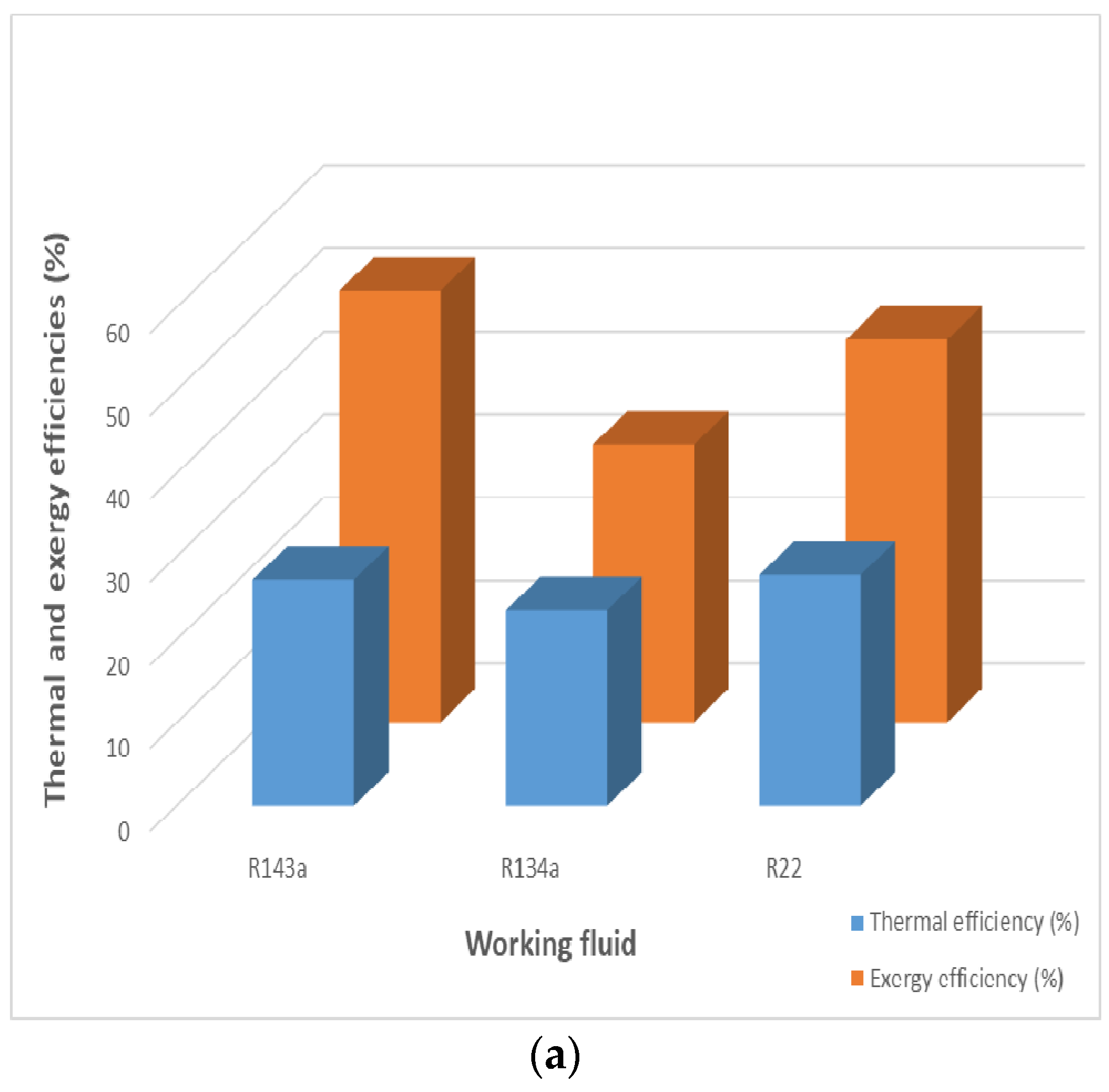
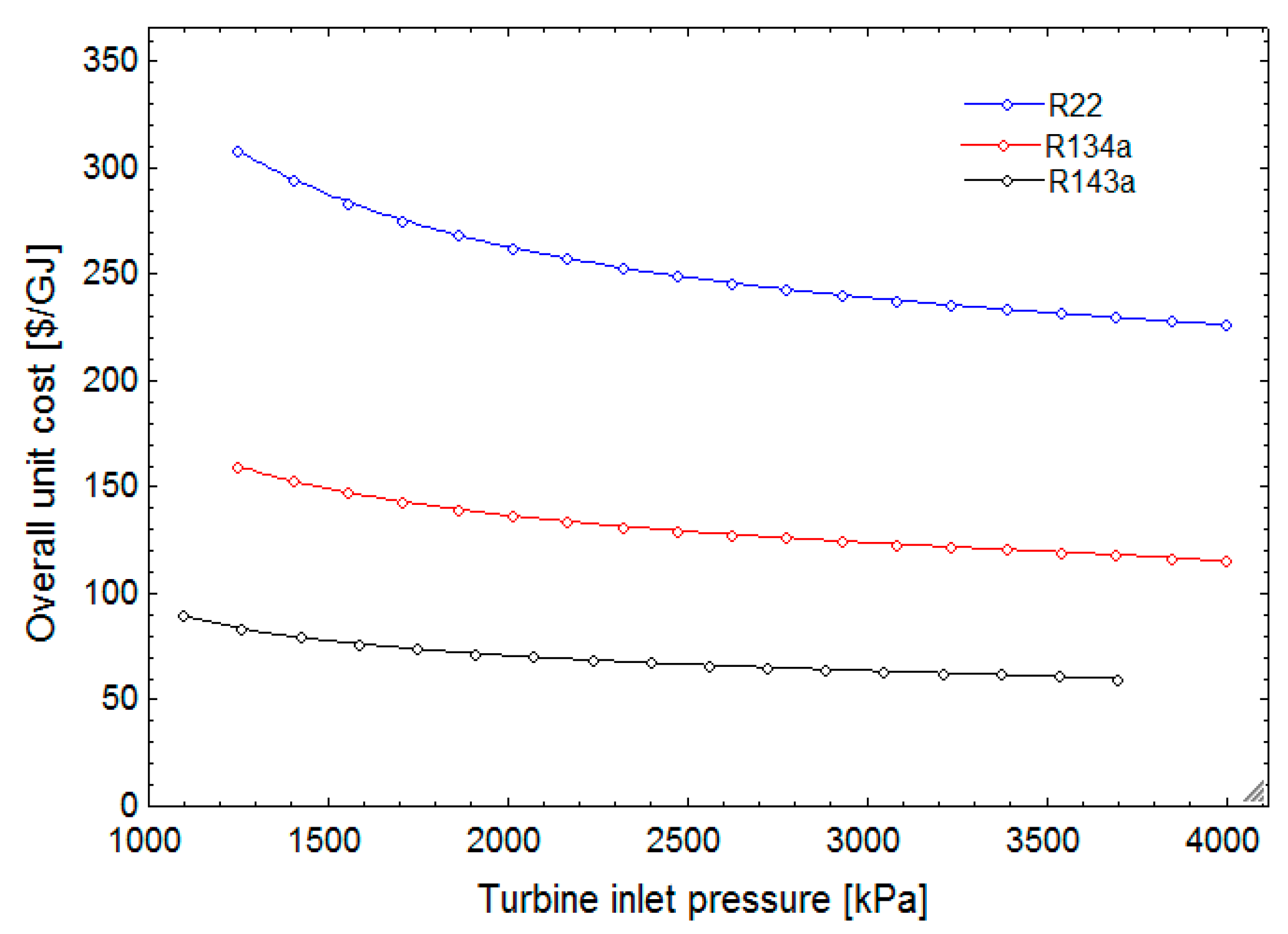
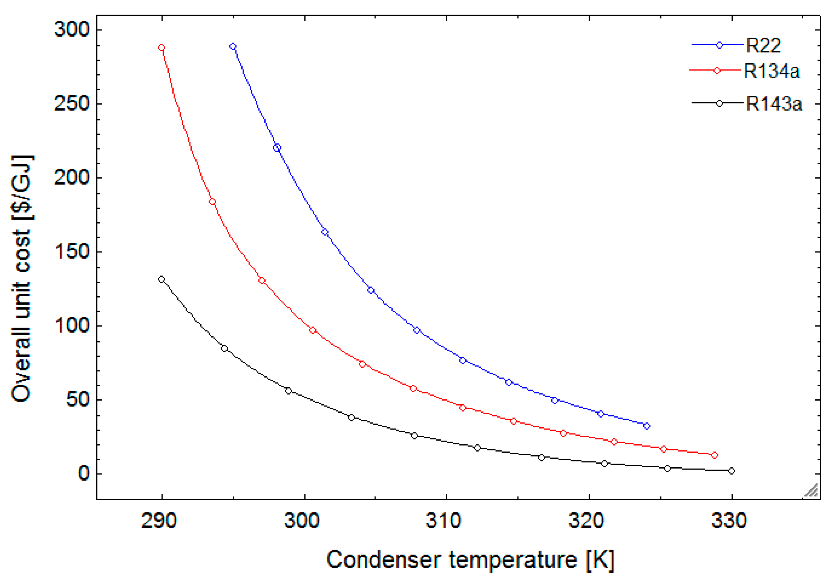
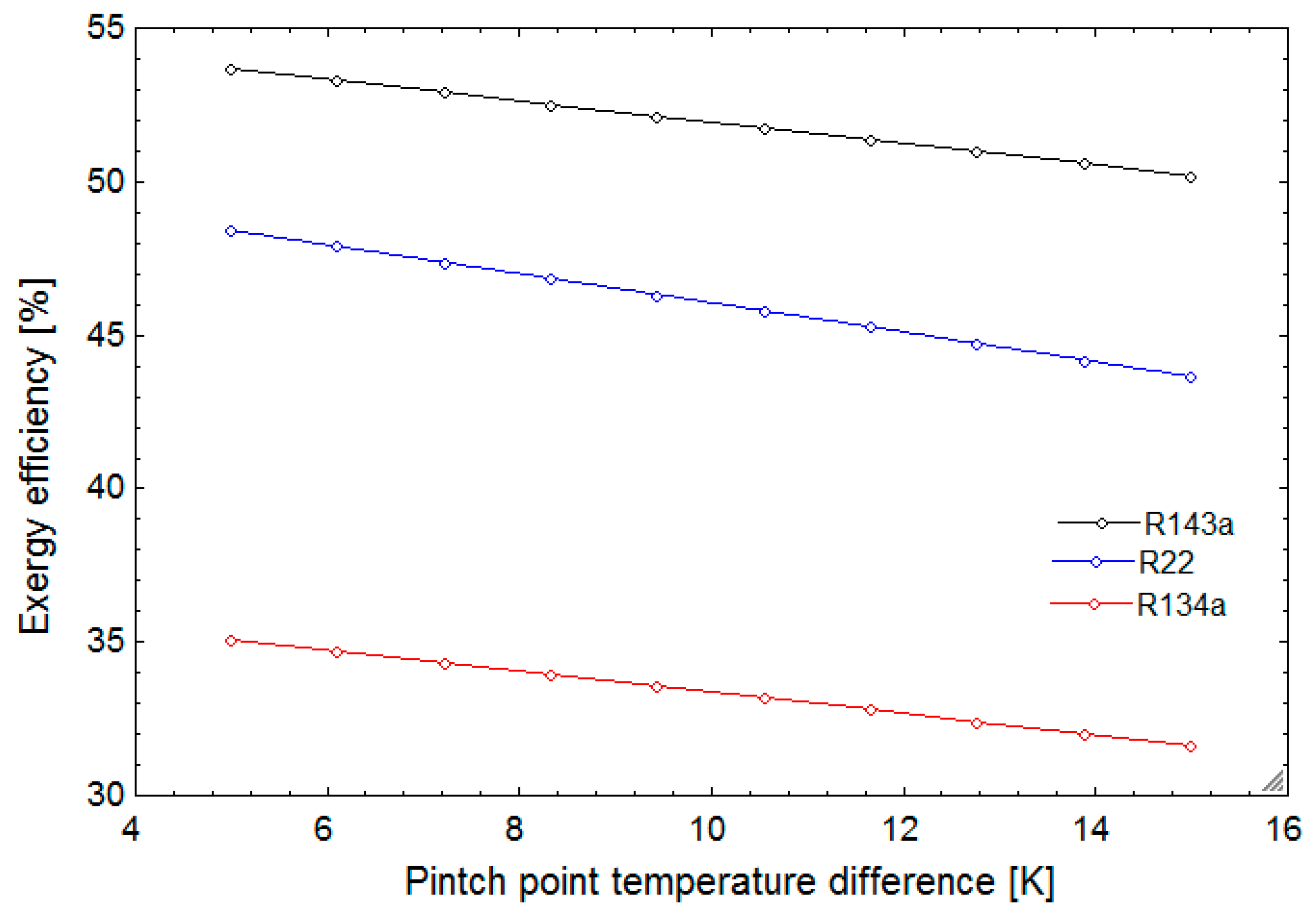
In this research, a combined cycle consisting of an ORC and a VCC using geothermal water as a low-temperature heat source is proposed and analyzed from thermodynamic and exergoeconomic viewpoints. The system generates electricity and cooling simultaneously. After determining the thermal and exergy efficiencies, a thermoeconomic analysis is performed to calculate each stream’s exergy cost, as well as total product unit cost of the system. Next, a parametric study is conducted to investigate the effects of decision parameters and various working fluids on the thermal and exergy efficiencies, as well as total product unit cost.

2. System Description

A schematic of the proposed cogeneration system is depicted in Figure 1. The system comprises two subsystems: an ORC producing power and a VCC to generate refrigeration. The two subsystems are connected in such a way that they have a common condenser, as shown in the figure.

Cooling water (geothermal) enters the condenser at temperature $T_{cw}$ (state 15) and the operating fluid exits as a saturated fluid at temperature $T_{cond}$ (state 6) and at the saturation pressure ($P_{cond}$), which represents the medium pressure of the system. The exiting stream from the condenser is then divided into two separate flows; one drives the ORC and the other passes through the VCC. In the VCC, after a decrease in its temperature and pressure in the throttle valve, the liquid is injected into the evaporator (state 10) and exits as a saturated vapor at temperature $T_e$ (state 11). Subsequently, the fluid is compressed by the compressor to pressure $P_{cond}$ (state 12) and is then mixed with the other flow from the ORC.

In the ORC, the pressure of the fluid from the condenser (state 7) is increased by the pump to the turbine inlet pressure ($P_h$), which is the highest pressure of the system. The outlet stream from the heat exchanger enters the boiler (state 1). Inside the boiler, thermal energy is supplied at temperature $T_s$; the fluid evaporates and is superheated to temperature $T_h$ at pressure $P_h$ (state 2). The fluid then enters the turbine where it undergoes an isentropic process, reaching pressure $P_{cond}$ and enters the heat exchanger (state 3). There, with the preheating of the input current of the heater from state 8 to 1, the flow temperature reduces from state 3 to 4. Next, the flows exiting the compressor and the heat exchanger, both at pressure $P_{cond}$, are mixed and then enter the condenser (state 5). It has been assumed that the minimum temperature difference between hot and cold flows in heat exchangers is greater than the described value of the pinch-point temperature difference ($\Delta T_{pp}$). The thermodynamic properties at points 3, 8, and 12 are obtained using expressions for the compressor, pump, and turbine isentropic efficiencies.

3. Modeling and Analyses

3.1. Thermodynamic Analysis

In order to evaluate the cycle thermodynamically, mass conservation laws as well as the first and second laws of thermodynamics were applied. Furthermore, energy and exergy relations were calculated using the EES software [20].

To simplify the calculations, the following assumptions were made regarding the cycle:

• The system is at steady state.
• The ambient temperature and pressure are 25 °C and 1014 Pa, respectively.
• Pressure drops in the system (heat exchangers and pipes) are negligible.
• Expansion and compression processes, in all compression and expansion components, are adiabatic.
• Changes in kinetic and potential energies are negligible.
• The fluid flow exiting the condenser is a saturated liquid.
• Outlet fluid from the evaporator is a saturated vapor.

A mass rate balance equation can be written as:

$${\displaystyle \sum {\dot{m}}_{in}=}{\displaystyle \sum {\dot{m}}_{out}}$$

(1)

Additionally, energy and exergy rate balances are given respectively by:

$${\displaystyle \sum {\dot{m}}_{in}{h}_{in}+{\dot{Q}}_{cv}-}{\displaystyle \sum {\dot{m}}_{out}}{h}_{out}-{\dot{W}}_{cv}=0$$

(2)

$${\displaystyle \sum {\dot{E}}_{in}-}{\displaystyle \sum {\dot{E}}_{out}+}{\displaystyle \sum {\dot{E}}_{heat}+}{\displaystyle \sum \dot{W}-\dot{I}=0}$$

(3)

The material exergy rate terms in the above equation for a component can be expressed as follows:

$${\dot{E}}_k=\dot{m}[(h-h_0)-T_0(s-s_0)]$$

(4)

where subscript ⁰ indicates the restricted dead state, which has the same temperature and pressure as the standard environment. Note that variations of other kinds of exergies like kinetic and chemical are neglected [21].

In cogeneration cycles, where there is more than one product, an energy utilization factor (EUF) can be defined instead of the thermal efficiency [22]:

$$EUF={\eta }_{thermal}=\frac{{\dot{W}}_{net}+{\dot{Q}}_{evaporator}}{{\dot{Q}}_{boiler}}*100$$

(5)

where ${\dot{W}}_{net}$ is the produced net power, which can be expressed as:

$${\dot{W}}_{net}={\dot{W}}_{turbine}-{\dot{W}}_{pump}-{\dot{W}}_{compressor}$$

(6)

and where ${\dot{Q}}_{evaporator}$ and ${\dot{Q}}_{boiler}$ are the heat transfer rates in the evaporator and the boiler. These can be expressed as follows:

$${\dot{Q}}_{evaporator}={\dot{m}}_{10}(h_{11}-h_{10})$$

(7)

$${\dot{Q}}_{boiler}={\dot{m}}_1(h_2-h_1)$$

(8)

Additionally, other performance criteria can be obtained from the following relations [23]. The relation for the second law efficiency can be expressed as follows:

$${\eta }_{exergy}=\frac{{\dot{E}}_{evaporator}+{\dot{W}}_{net}}{{\dot{E}}_{in}}*100$$

(9)

where ${\dot{E}}_{evaporator}$ and ${\dot{E}}_{in}$ are the exergy rates at the evaporator and the boiler, which can be written respectively as [21]:

$${\dot{E}}_{evaporator}={\dot{Q}}_{evaporator}(\frac{T_0}{T_{cs}}-1)$$

(10)

$${\dot{E}}_{in}={\dot{m}}_s{C}_{ps}(T_{air}-T_0-T_0\ln (\frac{T_{air}}{T_0}))$$

(11)

where $T_0$, $T_{cs}$, and $T_{air}$ are the environment, cooling space, and the ORC boiler inlet air temperatures, respectively. Additionally, ${\dot{m}}_s$ and $C_{ps}$ are, respectively, the mass flow rate and the specific heat capacity of the air entering the evaporator.

By applying the above equations for each component of the cycle depicted in Figure 1, detailed energy and exergy relations can be written, as shown in

Table 1. Energy and exergy relations for the proposed cycle.

Subsystem	Energy Relation	Exergy Analysis
Turbine	${\dot{m}}_8{h}_8={\dot{m}}_9{h}_9+{\dot{W}}_{turbine}$	${\dot{E}}_8={\dot{E}}_9+{\dot{W}}_{turbine}$
Mixer	${\dot{m}}_4{h}_4+{\dot{m}}_{10}{h}_{10}={\dot{m}}_5{h}_5$	${\dot{E}}_4+{\dot{E}}_{10}={\dot{E}}_5+{\dot{E}}_{destruction}$
Recuperator	${\dot{m}}_5{h}_5+{\dot{m}}_9{h}_9={\dot{m}}_{10}{h}_{10}+{\dot{m}}_7{h}_7$	${\dot{E}}_5+{\dot{E}}_9={\dot{E}}_7+{\dot{E}}_{10}+{\dot{E}}_{destruction}$
Boiler	${\dot{m}}_7{h}_7+{\dot{Q}}_{boiler}={\dot{m}}_8{h}_8$	${\dot{E}}_7+{\dot{E}}_{q,boiler}={\dot{E}}_5+{\dot{E}}_{destruction}$
Compressor	${\dot{m}}_3{h}_3={\dot{m}}_4{h}_4+{\dot{W}}_{compressor}$	${\dot{E}}_3={\dot{E}}_{11}+{\dot{W}}_{compressor}$
Condenser	${\dot{m}}_1{h}_1={\dot{Q}}_{condenser}+{\dot{m}}_5{h}_5$	${\dot{E}}_1+{\dot{E}}_{destruction}={\dot{E}}_{q,condenser}+{\dot{E}}_5$
Pump	${\dot{W}}_{pump=}{\dot{m}}_6(h_1-h_6)$	${\dot{E}}_1={\dot{E}}_6+{\dot{W}}_{pump}$
Evaporator	${\dot{m}}_2{h}_2+{\dot{Q}}_{evaporator}={\dot{m}}_3{h}_3$	${\dot{E}}_2+{\dot{E}}_{q,evaporator}={\dot{E}}_5+{\dot{E}}_{destruction}$

.

3.2. Thermoeconomic Analysis

The thermoeconomic analysis is a combination of exergy analysis and economics. Exergy analysis is capable of estimating exergy destruction values in components. In a thermoeconomic analysis, optimum conditions for the operation of the system can be obtained thermodynamically and economically by taking into account the thermodynamic and economic parameters simultaneously. The purpose of such an analysis is minimizing the cost of producing a product or maximizing the amount of product generated during a system’s operation with a fixed total cost.

For a thermodynamic system, there can be mass and energy flows at the inlet and the outlet, and exchanges of work and heat transfer with the environment. In accordance with mass and energy flows, exergy flows into and out of the system can occur. Additionally, due to system irreversibilities, there are exergy destructions. Since exergy represents the thermodynamic value of a flow, it is natural to relate the cost of these flows to their exergy transfer rates. This part of the thermoeconomics is called exergy costing. For each exergy stream in a system, the exergy cost rate ($\dot{C}$) and exergy unit cost rate ($\dot{c}$) can be defined.

The cost rate balance equation for each component of the system, receiving a heat transfer and generating power can be expressed as follows [21]:

$${\displaystyle \sum {\dot{C}}_{e,k}+}{\dot{C}}_{w,k}={\displaystyle \sum {\dot{C}}_{i,k}+{\dot{C}}_{q,k}}+{\dot{Z}}_k$$

(12)

where $\dot{Z}$ is the initial cost rate of each component, the indexes $i$ and $e$ represent the input and output flows, respectively, and ${\dot{C}}_q$ and ${\dot{C}}_w$, respectively, denote the cost rates associated with heat transfer and work rates. All the terms in the cost balance equation are positive, so that the cost rates associated with output exergies appear at the left side of the equation and those involved with input exergies are written at the right side. Then, the above equation can be rewritten as:

$${\displaystyle \sum {\dot{C}}_{e,k}+{\dot{c}}_{w,k}{\dot{W}}_k={\displaystyle \sum {\dot{C}}_{i,k}+{\dot{c}}_{q,k}{\dot{E}}_{q,k}+{\dot{Z}}_k}}$$

(13)

where

$${\dot{C}}_j={\dot{c}}_j{\dot{E}}_j$$

(14)

The cost balance and auxiliary equations for each component of the combined system considered in this study are listed in

Table 2. Cost rate balance and auxiliary equations for the components of the system.

Component	Cost Rate Balance	Auxiliary Equations
Turbine	${\dot{C}}_2+{\dot{Z}}_{turbine}={\dot{C}}_3+{\dot{C}}_{w,turbine}$	$c_{w,pump}=c_{w,turbine}$, $c_2=c_3$
Mixer	${\dot{C}}_4+{\dot{C}}_{12}={\dot{C}}_5$
Separator	${\dot{C}}_9+{\dot{C}}_7={\dot{C}}_6$	$c_7=c_9$
Boiler	${\dot{C}}_{air\_in}+{\dot{Z}}_{boiler}+{\dot{C}}_1={\dot{C}}_2+{\dot{C}}_{air\_out}$	$c_{air\_in}=c_{air\_out}$
Compressor	${\dot{C}}_{11}+{\dot{Z}}_{compressor}+{\dot{C}}_{w,compressor}={\dot{C}}_{12}$
Condenser	${\dot{C}}_5+{\dot{Z}}_{condenser}+{\dot{C}}_{15}={\dot{C}}_6+{\dot{C}}_{16}$	$c_5=c_6$, $c_{15}=0$
Pump	${\dot{C}}_7+{\dot{Z}}_{pump}+{\dot{C}}_{w,pump}={\dot{C}}_8$	$c_{w,pump}=c_{w,compressor}$
Evaporator	${\dot{C}}_{10}+{\dot{C}}_{13}+{\dot{Z}}_{evaporatpr}={\dot{C}}_{11}+{\dot{C}}_{14}$	$c_{11}=c_{10}$, $c_{13}=0$
Expansion valve	${\dot{C}}_9={\dot{C}}_{10}$

.

Economic Model and Analysis

The economic model estimates the purchased cost of equipment (initial cost) and operating and maintenance costs. In order to define a cost function that is dependent on the optimization parameters, the initial cost of each component of the system must be stated in terms of its thermodynamic characteristics. In the case of simultaneous power generation and refrigeration, we generally encounter three groups of components including turbines, pumps, and heat exchangers. The costs of these components can be expressed as follows [24]:

$$Z_{turbine}=C_{p,turbine}\times W_{turbine}^{0.7}$$

(15)

$$Z_{pump}=C_{p,pump}\times {[-\frac{W_{pump}}{100}]}^{0.26}\times {[1-\frac{{\eta }_{pump}}{{\eta }_{pump}}]}^{0.5}$$

(16)

$$Z_{HE}=C_{p,HE}\times {[\frac{A_{HE}}{100}]}^{0.6}$$

(17)

The values of bare module cost $(C_{p,k})$ for each of the components are listed in

Table 3. Values for the coefficients $(C_{p,k})$ for each component of the study system.

Subsystem	Bare Module Cost [$] $({\mathit{C}}_{\mathit{p},\mathit{k}})$
Turbine	$4405$
Heat exchanger	$16000$
Boiler	$17500$
Condenser	$16000$
Pump	$2100$
Evaporator	$16000$

[24].

Additionally, to estimate the heat transfer rates in the heat exchanger, the following equation is used:

$${\dot{Q}}_k=A_k{U}_k\Delta T_k^{lm}$$

(18)

where $U_k$, $A_k$, and $\Delta T_k^{lm}$ are, respectively, the total heat transfer coefficient, the heat transfer surface area, and the logarithmic mean temperature difference (LMTD). The relationships and values for LMTD and $U_k$ used in the present study are given in

Table 4. Relationships and values for logarithmic mean temperature difference (LMTD) and the total heat transfer coefficient ($U_k$).

Subsystem	Logarithmic Mean Temperature Difference $(\mathit{L}\mathit{M}\mathit{T}\mathit{D}{}_{\mathit{k}})$	Heat Transfer Coefficient ${\mathit{U}}_{\mathit{k}}(\frac{\mathit{W}}{{\mathit{m}}^2\mathit{K}})$
Heat exchanger	$LMT{D}_{he}=\frac{T_3-T_1-(T_4-T_8)}{\ln [\frac{T_3-T_1}{T_4-T_8}]}$	$1$
Boiler	$LMT{D}_{boiler}=\frac{T_{air}-T_2-(T_{air,out}-T_1)}{\ln [\frac{T_{air}-T_2}{T_{air,out}-T_1}]}$	$0.9$
Evaporator	$LMT{D}_{eva}=\frac{T_{13}-T_{11}-(T_{14}-T_{10})}{\ln [\frac{T_{13}-T_{11}}{T_{14}-T_{10}}]}$	$1.5$
Condenser	$LMT{D}_{cond}=\frac{T_5-T_{16}-(T_6-T_{15})}{\ln [\frac{T_5-T_{16}}{T_6-T_{15}}]}$	$1.1$

.

To calculate the levelized capital investment cost for a component, the following general relation is used [24]:

$${\dot{Z}}_k=\frac{CRF\times Z_k+\beta \times Z_k}{\tau }$$

(19)

Here $\tau$ denotes the annual operation hours for a plant in one year. Additionally, CRF is the capital recovery factor for a system, expressible as follows [20,21]:

$$CRF=\frac{i_r{(1+i_r)}^n}{{(1+i_r)}^n-1}$$

(20)

where $i_r$ is the annual interest rate and n is the plant useful operation life.

To bring the cost of system components to the reference year, the chemical engineering plant cost index (CEPCI) and the following relation are used [21]:

$$\mathrm{cost}\mathrm{at}\mathrm{reference}\mathrm{year}=\mathrm{original}\mathrm{cost}?\frac{\mathrm{cost}\mathrm{index}\mathrm{for}\mathrm{the}\mathrm{reference}\mathrm{year}}{\mathrm{cost}\mathrm{index}\mathrm{for}\mathrm{the}\mathrm{original}\mathrm{year}}$$

(21)

4. Results

To verify the validity of the results, a study by Kim and Perez-Blanco [10] was used. In that research, a thermodynamic analysis of a cycle involving the simultaneous generation of power and refrigeration with a low-temperature energy source was considered. The cycle included an ORC for power generation and a VCC for producing refrigeration, including limited generation of cooling without producing electricity, and used the same operating fluid with the ORC. For validation, the variation of thermal efficiency with changes in the turbine inlet pressure for the R143a working fluid was plotted and compared with the obtained graph in this study. As shown in Figure 2, the results were in good agreement with the results obtained from Kim and Perez-Blanco’s work [10].

Performance Results

The values of the initial input data and results for the cogeneration cycle and for the proposed cycle are presented in

Table 5. Initial conditions and input data.

Parameter	Value
Source temperature	$T_S=150°C$
Cooling water temperature	$T_{cw}=25°C$
Condenser temperature	$T_{cond}=25°C$
Condenser pressure	$P_{cond}=1000kPa$
Dead state temperature	$T_0=25°C$
Environment pressure	$P_0=101kPa$
Pinch-point temperature difference	$\Delta T_{pp}=10°C$
Refrigeration space temperature	$T_{cs}=15°C$
Evaporator temperature	$T_e=5°C$
Plant useful life	$n=20years$
Annual interest rate	$i_r=15\%$
Plant annual operation hours	$\tau =8000\raisebox{1ex}{$h$}\!\left/ \!\raisebox{-1ex}{$year$}\right.$
Fluid mass flow rate	${\dot{m}}_{ref}=60\raisebox{1ex}{$kg$}\!\left/ \!\raisebox{-1ex}{$s$}\right.$
Boiler mass flow rate (air)	${\dot{m}}_{boiler}=100\raisebox{1ex}{$kg$}\!\left/ \!\raisebox{-1ex}{$s$}\right.$
Turbine inlet pressure	$P_h=3600kPa$
Condenser inlet water temperature	$T_{water,in}=15°C$
Pump isentropic efficiency	${\eta }_{pump}=0.8$
Turbine isentropic efficiency	${\eta }_{turbine}=0.8$
Compressor isentropic efficiency	${\eta }_{compressor}=0.8$

and

Table 6. Numerical results of modeling the proposed cycle operating with R143a.

State	${\dot{\mathit{m}}}_{\mathit{i}}$ (Mass Flow Rate) [kg/s]	${\mathit{T}}_{\mathit{i}}$ (Temperature) [K]	${\mathit{P}}_{\mathit{i}}$ (Pressure) [kPa]	${\mathit{h}}_{\mathit{i}}$ (Enthalpy) [kJ/kg]	${\mathit{s}}_{\mathit{i}}$ (Entropy) [kJ/kg-K]	${\mathit{e}}_{\mathit{i}}$ (Exergy) [kW]	${\dot{\mathit{c}}}_{\mathit{i}}$ (Product Unit Cost) [$/GJ]	${\dot{\mathit{C}}}_{\mathit{i}}$ (Product Cost) [$/h]
1	50	338.4	3600	314.4	1.362	3788	70.08	955.6
2	50	430.1	3600	537.3	1.971	5854	46.09	971.4
3	50	382.1	1000	501.5	1.995	3712	46.09	615.9
4	50	318.8	1000	429.8	1.79	3184	46.09	528.4
5	60	314.4	1000	424.8	1.774	3803	67.59	925.5
6	60	298.2	1000	239.2	1.135	4094	67.59	996.1
7	50	298.2	1000	239.2	1.137	3387	68.09	830.1
8	50	300.9	3600	242.7	1.138	3537	68.14	867.5
9	10	298.2	1000	239.2	1.137	677.3	68.09	166
10	10	278.1	722.3	239.2	1.027	1004	45.94	166
11	10	278.2	722.3	390.3	1.684	556.2	45.94	91.98
12	10	292.8	1000	399.5	1.69	629.6	175.2	397.1

. Applying the values presented in this table, as well as the relationships provided for energy, exergy, and economic analyses in the previous sections, the values are determined for pressure, temperature, operating fluid (R143a) flow rate, exergy rate, exergy unit cost rate, and exergy cost rate. The results are presented in Table 6 and

Table 7. Performance results for the proposed cycle.

Parameter		Value
$EUF={\eta }_{thermal}$	Thermal efficiency	$27.21\%$
${\eta }_{exergy}$	Exergy efficiency	$51.95\%$
${\dot{W}}_{net}$	Net power	$1523kW$
${\dot{Q}}_{evaporator}$	Evaporator heat rate	$1511kW$
${\dot{E}}_{evaporator}$	Evaporator exergy rate	$13.34kW$
${\dot{c}}_{p,overall}$	Total product unit cost	$60.75\raisebox{1ex}{$\$$}\!\left/ \!\raisebox{-1ex}{$GJ$}\right.$

.

Figure 3 depicts the percentage of exergy destruction for each component in the cogeneration cycle using R143a. It is evident that the boiler and turbine contribute the most to the exergy destruction, while the compressor and mixer contribute the least.

A comparison between different working fluids regarding their effects on the thermal and exergy efficiencies, total product unit cost, total exergy destruction rate, cooling capacity, and produced net power is depicted in Figure 4. It is apparent that the system has the highest energy and exergy efficiencies as well as the lowest total production unit cost when using R143a. Furthermore, a higher exergy destruction rate for the case of using R22 results in the highest production cost.

5. Parametric Study

In this section, a parametric analysis is carried out to investigate the effects of several parameters on the cycle performance. The results of variations in several decision parameters are presented.

5.1. Effect of Turbine Inlet Pressure (TIP)

The variation of first law efficiency with TIP in the cogeneration cycle is depicted in Figure 5 for three working fluids. As can be seen, the thermal efficiency rose consistently with increasing TIP in all cases. Furthermore, for a given value of TIP in Figure 5, the systems using R22 and R134a exhibited the highest and lowest thermal efficiencies, respectively.

Similarly, the variation of the exergy efficiency with TIP for the proposed system is depicted in Figure 6 for the same working fluids. Like the trend depicted in Figure 5, the exergy efficiency increased with increasing TIP. Additionally, the systems using R143 and R134 exhibited the highest and lowest exergy efficiencies, respectively. By comparing Figure 5 and Figure 6, it is evident that the system using R134a had the lowest energy and exergy efficiencies among other working fluids, whereas the systems using R22 and R143a had the highest first and second law efficiencies, respectively.

The trends depicted in Figure 5 and Figure 6 can be justified by considering Equations (5) and (9). For constant values of ${\dot{Q}}_{evaporator}$ and ${\dot{Q}}_{boiler}$ as well as ${\dot{E}}_{evaporator}$ and ${\dot{E}}_{in}$, the variation of ${\dot{W}}_{net}$ with TIP, as shown in Figure 7, justified the trends indicated in Figure 5 and Figure 6. It is apparent that the cycle produced the least and most power while working with R134a and R143a, respectively.

Figure 8 illustrates the trend for exergy destruction ratio in each component as TIP varies, for the system with R143 as the working fluid. It is evident that, while the TIP rose, the heat exchanger exergy destruction ratio varied negligibly. This ratio for the turbine, condenser, and evaporator increased with increasing TIP, while for the boiler a downward trend was observed. Additionally, the heat exchanger and boiler had the lowest and highest exergy destruction ratios, respectively.

The variation of $c_{p,total}$ with TIP is depicted in Figure 9. It is seen that, for all mentioned working fluids, $c_{p,total}$ decreased as TIP increased. Additionally, $c_{p,total}$ was the lowest and highest for R143a and R22, respectively. It is evident that the greatest cost reduction occurred when the cycle ran with R22 as the TIP increases. Additionally, it is important to note that varying TIP did not have a significant effect on $c_{p,total}$.

5.2. Effect of Condenser Pressure ($P_{cond}$)

The variations of the first and second law efficiencies with condenser pressure are illustrated in Figure 10 and Figure 11, respectively. It is evident that both efficiencies decrease with increasing $P_{cond}$. The results in Figure 5 and Figure 6 as well as Figure 10 and Figure 11 are congruent, as an increase in the pressure difference across the turbine bought about higher thermal and exergy efficiencies that were expected.

Similar to the previous section, the variations of first and second law efficiencies, as depicted in Figure 10 and Figure 11, respectively, are justified considering the results in Figure 12.

5.3. Effect of Condenser Temperature ($T_{cond}$)

In this section, the effect of varying $T_{cond}$ is investigated on the total product unit cost of the system and the results are shown in Figure 13. It is apparent that the systems using R143a and R22 have the greatest and lowest costs, respectively. Additionally, for all working fluids, $c_{p,total}$ reaches a minimum with increasing condenser temperature.

5.4. Effect of Pinch-Point Temperature Difference ($\Delta T_{pp}$)

In this section, the effect of $\Delta T_{pp}$ on system performance was studied. A descending trend is observed for both the first and second law efficiencies with increasing pinch-point temperature difference, as seen in Figure 14 and Figure 15. The trend can be explained by observing the effect of $\Delta T_{pp}$ on the ${\dot{W}}_{net}$ (Figure 16), and considering Equations (5) and (9).

6. Conclusions

In the present study, thermodynamic and exergoeconomic analyses are carried out on a novel combined cycle comprised of vapor-compression refrigeration and organic Rankine cycles. The governing relationships for the combined cycle are expressed using the laws of mass and energy conservation and exergy analysis, and relations for exergoeconomic analysis are given. The effects are investigated of varying numerous parameters on cycle performance measures, like first and second law efficiencies, total product unit cost, produced net power, and component exergy destruction ratios. The conclusions that can be drawn from the results are as follows:

• The proposed configuration is proved to be an efficient cogeneration system.
• The largest exergy destruction occurs in the boiler and turbine, respectively.
• Among the three working fluids, the R143a has the best result from the viewpoint of both the second law of thermodynamics and economics.
• The highest product unit cost is achieved with R22 as the working fluid.
• Better thermodynamic and economic results are achieved with higher turbine inlet pressure and lower condenser pressure as well as lower pinch-point temperature difference.
• Increasing TIP results in an increase in all component exergy destruction ratios, except the boiler. The net change in exergy destruction; however, is negative because the boiler is dominant in this respect.

References

1. Hammad, A.; Dincer, I. Analysis and assessment of an advanced hydrogen liquefaction system. Int. J. Hydrogen Energy 2018, 43, 1139–1151. [Google Scholar] [CrossRef]
2. Islam, S.; Dincer, I.; Yilbas, B.S. System development for solar energy-based hydrogen production and on-site combustion in HCCI engine for power generation. Sol. Energy 2016, 136, 65–77. [Google Scholar] [CrossRef]
3. Bertani, R. Geothermal power generation in the world 2010–2014 update report. Geothermics 2016, 60, 31–43. [Google Scholar] [CrossRef]
4. Lucia, U.; Simonetti, M.; Chiesa, G.; Grisolia, G. Ground-source pump system for heating and cooling: Review and thermodynamic approach. Renew. Sustain. Energy Rev. 2017, 70, 867–874. [Google Scholar] [CrossRef]
5. Zhang, Z.; Alelyani, S.; Zhang, N. Thermodynamic analysis of a novel sodium hydroxide-water solution absorption refrigeration, heating and power system for low-temperature heat sources. Appl. Energy 2018, 222, 1–12. [Google Scholar] [CrossRef]
6. Marco, A.; Dario, A.; Silvia, L.; Ennio, M. Comparison between ORC and CO2 power systems for the exploitation of low-medium temperature heat sources. Energy 2018, 161, 1250–1261. [Google Scholar]
7. Sun, W.; Yue, X.; Wang, Y. Exergy efficiency analysis of ORC (Organic Rankine Cycle) and ORC based combined cycles driven by low-temperature waste heat. Energy Convers. Manag. 2017, 135, 63–73. [Google Scholar] [CrossRef]
8. Arora, C.P. Refrigeration and Air Conditioning, 3rd ed.; Tata McGraw-Hill: New Delhi, India, 1981. [Google Scholar]
9. Palagia, L.; Sciubbab, E.; Toccib, L. A neural network approach to the combined multi-objective optimization of the thermodynamic cycle and the radial inflow turbine for Organic Rankine cycle applications. Appl. Energy 2019, 237, 210–226. [Google Scholar] [CrossRef]
10. Kim, K.; Perez-Blanco, H. Performance analysis of a combined organic Rankine cycle and vapor compression cycle for power and refrigeration cogeneration. Appl. Therm. Eng. 2015, 91, 964–974. [Google Scholar] [CrossRef]
11. Moles, F.; Navarro-Esbri, J.; Peris, B.; Mota-Babiloni, A. Thermodynamic analysis of a combined organic Rankine cycle and vapor compression cycle system activated with low-temperature heat sources using low GWP fluids. Appl. Therm. Eng. 2015, 87, 444–453. [Google Scholar] [CrossRef]
12. Wall, G. Thermoeconomic optimization of a heat pump system. Energy 1986, 11, 957–967. [Google Scholar] [CrossRef] [Green Version]
13. Karellas, S.; Braimakis, K. Energy-exergy analysis and economic investigation of a cogeneration and trigeneration ORC-VCC hybrid system utilizing biomass fuel and solar power. Energy Convers. Manag. 2016, 107, 103–113. [Google Scholar] [CrossRef]
14. Toujeni, N.; Bouaziz, N.; Kairaouani, L. Energetic investigation of a new combined ORC-VCC system for cogeneration. Energy Procedia 2017, 139, 670–675. [Google Scholar] [CrossRef]
15. Vasta, S.; Palomba, V.; La Rosa, D.; Mittelbach, W. Adsorption-compression cascade cycles: An experimental study. Energy Convers. Manag. 2018, 156, 365–375. [Google Scholar] [CrossRef]
16. Mirzaei, M.; Ahmadi, M.H.; Mobin, M.; Nazari, M.A.; Alayi, R. Energy, exergy and economics analysis of an ORC working with several fluids and utilizes smelting furnace gases as heat source. Therm. Sci. Eng. Prog. 2018, 5, 230–237. [Google Scholar] [CrossRef]
17. Konstantinos, B.; Sotirios, K. Exergetic optimization of double stage Organic Rankine Cycle (ORC). Energy 2018, 149, 296–313. [Google Scholar]
18. Chang, H.; Wan, Z.; Zheng, Y.; Chen, X.; Shu, S.; Tu, Z.; Chan, S.H. Energy analysis of a hybrid PEMFC-solar energy residential micro-CCHP system combined with an organic Rankine cycle and vapor compression cycle. Energy Convers. Manag. 2017, 142, 374–384. [Google Scholar] [CrossRef]
19. Javaherdeh, K.; Alizadeh, A.; Zoghi, M. Simulation of combined steam and organic Rankine cycle from energy and exergoeconomic point of view with exhaust gas source. Modares Mech. Eng. 2016, 16, 308–316. [Google Scholar]
20. Klein, S.A.; Alvarado, S.F. Engineering Equation Solver (EES); F-chart Software: Madison, WI, USA, 2007. [Google Scholar]
21. Bejan, A.; Tsatsaronis, G.; Moran, M. Thermal Design and Optimization; John Wiley and Sons: New York, NY, USA, 1996. [Google Scholar]
22. Puig-arnavat, M.; Bruno, J.C.; Coronas, A. Modeling of trigeneration configurations based on biomass gasification and comparison of performance. Appl. Energy 2014, 114, 845–856. [Google Scholar] [CrossRef]
23. Akbari, M.; Mahmoudi, S.M.S. Exergeoconomic analysis and optimization of a novel cogeneration system producing power and refrigeration. Energy Conserv. Manag. 2017, 134, 208–220. [Google Scholar] [CrossRef]
24. Kazemi, N.; Samadi, F. Thermodynamic, economic and thermo-economic optimization of a new proposed organic Rankine cycle for energy production from geothermal resources. Energy Convers. Manag. 2016, 121, 391–401. [Google Scholar] [CrossRef]
Figure 1. Schematic of the combined cycle considered in the present study.
Sustainability 11 03374 g001
Figure 2. Comparison between the results obtained in the present work with those reported by Kim and Perez-Blanco [10].
Sustainability 11 03374 g002
Figure 3. Component exergy destruction ratios of the proposed cycle.
Sustainability 11 03374 g003
Figure 4. Effects of different working fluids on (a) thermal and exergy efficiencies, (b) total production unit cost, (c) total exergy destruction rate, (d) cooling capacity, and (e) produced net power.
Sustainability 11 03374 g004aSustainability 11 03374 g004bSustainability 11 03374 g004c
Figure 5. Effect of varying turbine inlet pressure (TIP) on thermal efficiency for several working fluids.
Sustainability 11 03374 g005
Figure 6. Effect of varying TIP on exergy efficiency for several working fluids.
Sustainability 11 03374 g006
Figure 7. Effect of varying TIP on produced net power.
Sustainability 11 03374 g007
Figure 8. Effect of varying TIP on component exergy destruction ratios.
Sustainability 11 03374 g008
Figure 9. Effect of varying TIP on total product unit cost.
Sustainability 11 03374 g009
Figure 10. Effect of varying condenser pressure ( P c o n d ) on thermal efficiency.
Sustainability 11 03374 g010
Figure 11. Effect of varying condenser pressure ( P c o n d ) on exergy efficiency.
Sustainability 11 03374 g011
Figure 12. Effect of varying condenser pressure ( P c o n d ) on net power.
Sustainability 11 03374 g012
Figure 13. Effect of varying condenser temperature ( T c o n d ) on total product unit cost.
Sustainability 11 03374 g013
Figure 14. Effect of varying Pinch-Point Temperature Difference ( Δ T p p ) on thermal efficiency.
Sustainability 11 03374 g014
Figure 15. Effect of varying Pinch-Point Temperature Difference ( Δ T p p ) on exergy efficiency.
Sustainability 11 03374 g015
Figure 16. Effect of varying Pinch-Point Temperature Difference ( Δ T p p ) on net power ( W ˙ n e t ) .
Sustainability 11 03374 g016