Article

Balancing Population Distribution and Sustainable Economic Development in Yangtze River Economic Belt of China

1
School of Public Administration, Zhongnan University of Economics and Law, Wuhan 430073, China
2
Center for Environment and Migration Studies, Zhongnan University of Economics and Law, Wuhan 430073, China
3
College of Environment and Planning, Henan University, Kaifeng 475001, China
4
Department of Geography, Kent State University, Kent, OH 44240, USA
*
Author to whom correspondence should be addressed.
Sustainability 2019, 11(12), 3320; https://doi.org/10.3390/su11123320
Submission received: 9 May 2019 / Revised: 9 June 2019 / Accepted: 13 June 2019 / Published: 16 June 2019
(This article belongs to the Section Economic and Business Aspects of Sustainability)

Abstract

:
From a macro perspective, the inconsistency between population distribution and economic development reflects the lag of population mobility and, at the same time, widens regions’ economic disparity. China, as a socialist country, is very concerned with the regional disparities. Aiming at analyzing ways to reduce regional disparities and promote balanced and sustainable regional developments, this paper applies spatial analytical methods in econometrics, using the Yangtze River Economic Belt in China as an example, to analyze the spatial inconsistency between the distribution of population and economic development. The study also examines the influencing factors for such inconsistency and proposes countermeasures from the perspective of floating population and regional economics. The research results show that the improvement of human capital and the tilt of regional policies are conducive to population agglomeration. Furthermore, increasing the input of physical capital can promote economic agglomeration. From the spatial econometric analysis in this paper, the direct and indirect effects have opposite directions, so it is necessary to consider the indirect effects when implementing policies or programs.

1. Introduction

Williamson [1] applied the inverse U-shaped curve of the distribution of income in Kuznets [2] to the analysis of regional economies. Specifically, it proposed the inverted U theory to explain regional economic disparities. Williamson indicated that differences among regions in a country often showed a U-shape trend of changes against the improvement of economic development levels, i.e., regional differences typically decline first and then rise after reaching the bottom of the trend against economic development. The New Geo-Economics [3,4,5,6,7,8,9,10] explains that economic gathering of goods and services determines how population and capital flow spatially. These flow processes themselves tend to continuously self-strengthen. This often results in different industries concentrating to different degrees on the inflows of population and capitals in a circular causal mechanism that is gradually formed over time.
From a macro perspective, the inconsistency between population distribution and economic development reflects the lag of population mobility to a certain extent and, at the same time, widens regional economic disparities. To further explore this inconsistency, the objective of this paper is to analyze how to reduce regional disparities and promote balanced and sustainable developments among regions. Based on spatial econometrics methods, this paper also analyzes how the two forces of the market and the government together influence the intra-/inter-regional inconsistency between population distribution and economic development so as to explore policy implications for how to promote a consistent distribution between them with regard to controllable factors and for reducing regional disparities.
The study area of this paper is the Yangtze River Economic Belt (YREB) of China. In 2014, China included YREB in national strategies for economic development. In 2016, China released a development outline for YREB. It also made the development of YREB to be a top priority across all sectors of the society. The coordinated distribution of population and economic landscape in YREB is the key to a balanced and sustainable development of China.
The limitations of the existing literature [11,12,13,14,15,16] are mainly in two aspects. First, there is no theoretical explanation for the relationship between population distribution and economic development inconsistency and regional imbalance in economic development. Second, the interaction between regions is often not considered in existing studies. The contribution of this paper is three-fold. First, this paper provides a theoretical explanation for the inconsistency between population distribution and economic development by quantitatively measuring regional disparities with potential influencing factors. Second, this paper considers the inter-regional interactions from a spatial perspective that recognizes the different regional characteristics. Finally, this paper aims at promoting a balanced and sustainable approach to regional economic development. It recognizes that, as a socialist country, China requires the realization of balanced and sustainable development. Given this, China is by default very concerned with the regional disparities. Consequently, it has successively introduced strategies for such purposes, including the revitalization of the Northeast, the promotion for the rise of the central region, the development of the western region, and the coordinated development of urban and rural areas. These concerns and supports are all important national strategies for narrowing the regional gaps and reducing poverty. To that end, this paper also explores whether it is possible to narrow the regional gaps from a macroeconomic perspective of governmental regulations through the study of YREB.
In the subsequent sections, Section 2 reviews relevant literature on regional disparities, their measurements as linked to population distribution, and economic development and how the influencing factors function. Section 3 introduces data and methods used in the study, including a discussion of the model constructed here. Section 4 analyzes results from testing the significance of spatial autocorrelation of the model variables, the selection of model variables, and the empirical results from the constructed spatial econometric models. The final section concludes the paper and offers recommendations for policy makers and future researchers.

2. Consistency of Population and Economy (CPE) and Regional Economic Disparity

On measuring regional economic disparities, there exist studies carried out using simple indicators such as Gini, Theil and Atkinson indices [17]. There also exist others that used per capita gross domestic product (PCGDP) and per capita income (PCI) for exploring regional economic disparities [18]. This paper chose to apply the index of consistency of population and economy (CPE) to gauge regional economic disparities. CPE is an important indicator which indicates the degree of consistency between the population distribution and economic development of a region [11,12,14]. There are relatively few studies that use CPE to measure region disparities, but those did show that inconsistency between the population distribution and economic development tend to enlarge regional disparities [15,19].
Since China’s economic reform in 1978, migration has become an important factor influencing population distribution. According to China’s Floating Population Development Report 2018 [20], the migration of population from labor-intensive industries to capital- and technology-intensive industries was recognized as conducive to the coordinated development of regional industries, thereby promoting economic growth.
The flows of the population from central and western regions to the eastern regions have for a long time reflected the comparative advantages of capital-intensive or technology-intensive industries over labor-intensive industries in the coastal regions. However, some of China’s labor force, especially migrant workers, was found to have recently returned from the eastern coastal areas to the central and western regions. This is because labor-intensive industries and resource-intensive industries in China have shifted to the central and western regions from coastal regions.
The process of population flowing with industrial transformation is known to promote an optimal allocation of human capital between regions and increase labor productivity [21]. Given this, changes in the distribution of population could consequently promote economic development. Some studies have pointed out that the existence of regional differences may be the reason for causing population migration. Retrospectively, the inconsistency in the spatial distribution of population and economic development, in turn, reflects, to some extent, the existence of regional differences, and at the same time indicates the lag and mismatch of population flows.
China Mobile Population Development Report 2018 also sorts out China’s floating population policies over the past 40 years. The report summarizes the changing policies into three phases. The first phase was from 1984 to 2002, which was the gradual liberalization of population mobility. The second phase was from 2003 to 2012, it was identified as the period that fair policies for the floating population being proposed and implemented. The third stage was from 18th National Congress of the Communist Party of China in 2003, which comprehensively promoted the citizenization (Citizenization is the process through which floating population become city residents and enjoy the same public service system as local residents in cities.) stage of the floating population. Therefore, by exploring the inconsistency in the spatial distribution of population and economic development, the effectiveness of China’s floating population policy has also been tested to some extent.
According to the growth pole theory [22], there are two effects of polarization and diffusion of regional economic development. If the resources are properly configured, the network-balanced development pattern between regions can be realized. According to the inverted U-shaped economic development theory, Williamson believes that in the initial stage of economic development, the regional economic development gap is constantly expanding, but after a certain period of time, the balance of developmental forces would make the regional gap stable. After entering the maturity stage, the regional gap would gradually decrease with the overall growth. Therefore, the inconsistency of the spatial distribution of population and economy could exist for a long time with possible volatility.
According to regional development theory [23,24,25], regional development policies have often over-emphasized the promotion of regional economic prosperity, which tended to lead to an over-reliance on public assistance in regions and underestimated their potential roles of promoting the mobility of the population and other resources in the regions. What is important for a region’s development is its interdependence of activities and interests with other regions and how the changes in one activity may have external and neighborhood effects on other activities. Guided by these conceptual foundations, this paper explores ways to promote effective allocations of resources and promote the free flows of resources for balanced and sustainable regional economic development.

3. Data and Methods

3.1. Research Data

The data used in this research came from China Regional Statistical Yearbooks and the statistical yearbooks of provinces in YREB over the study years. Due to some changes in the administrative divisions of the cities from 1999 to 2013, the spatial data and the names of the cities in the yearbooks were sorted and adjusted according to the administrative divisions in 2010 to maintain consistency among data sets.
YREB covers the eastern, central, and western regions of China, with the combined population and economic worth exceeding 40% of the country. It is no doubt a large economy. The disparities among regions in YREB are great and significant. Specifically, the level of population agglomeration lags that of economic agglomeration. There are apparent imbalance and mis-matches between the population distribution and economic development in YREB. Such imbalance would hinder the green development (Green development is the way of economic growth and social development with the goal of efficiency, harmony, and sustainability. Green development is attracting attention in China and the world at present.) in YREB. Figure 1a shows the distribution of the population in YREB in 2013, Figure 1b shows the distribution of the economic product in GDP in YREB in 2013. It can be seen that there are almost always high population and economic development in capital cities of all provinces in YREB. Comparing the two figures, the two distributions are not obviously different. They show that the regional disparities in economic development are more significant than that in the population distribution in YREB.
Regional imbalance and mismatches between population and economic development can be the roots for the stagnant development in regions that are lagging behind. It would be important to assess the level of such imbalance and mismatches so that effective strategies and intervention programs or policies can be developed to address these issues.

3.2. CPE Values Index

The CPE index is defined as the ratio of economic concentration to population concentration. It is an important indicator that indicates the degree of consistency between the population distribution and economic development in a region. The formula used to calculate values of CPE is as the following:
CPE i t = g i t i = 1 n g i t p i t i = 1 n p i t
where git is the gross domestic product (GDP) in the region i at time t, pit is the population in the region i at time t.
When the value of CPE for a region is found to be greater than 1, the population concentration is less than the economic concentration of the region, and vice versa. When the value of CPE is equal to 1, it means the population concentration is at the same level as that of the economic concentration. The economic concentration ratio is the ratio of the economic product shares in the region i at time t to the whole economic product in all regions at time t. The population concentration ratio is the ratio of the population shares in the region i at time t to the whole population in all regions at time t.
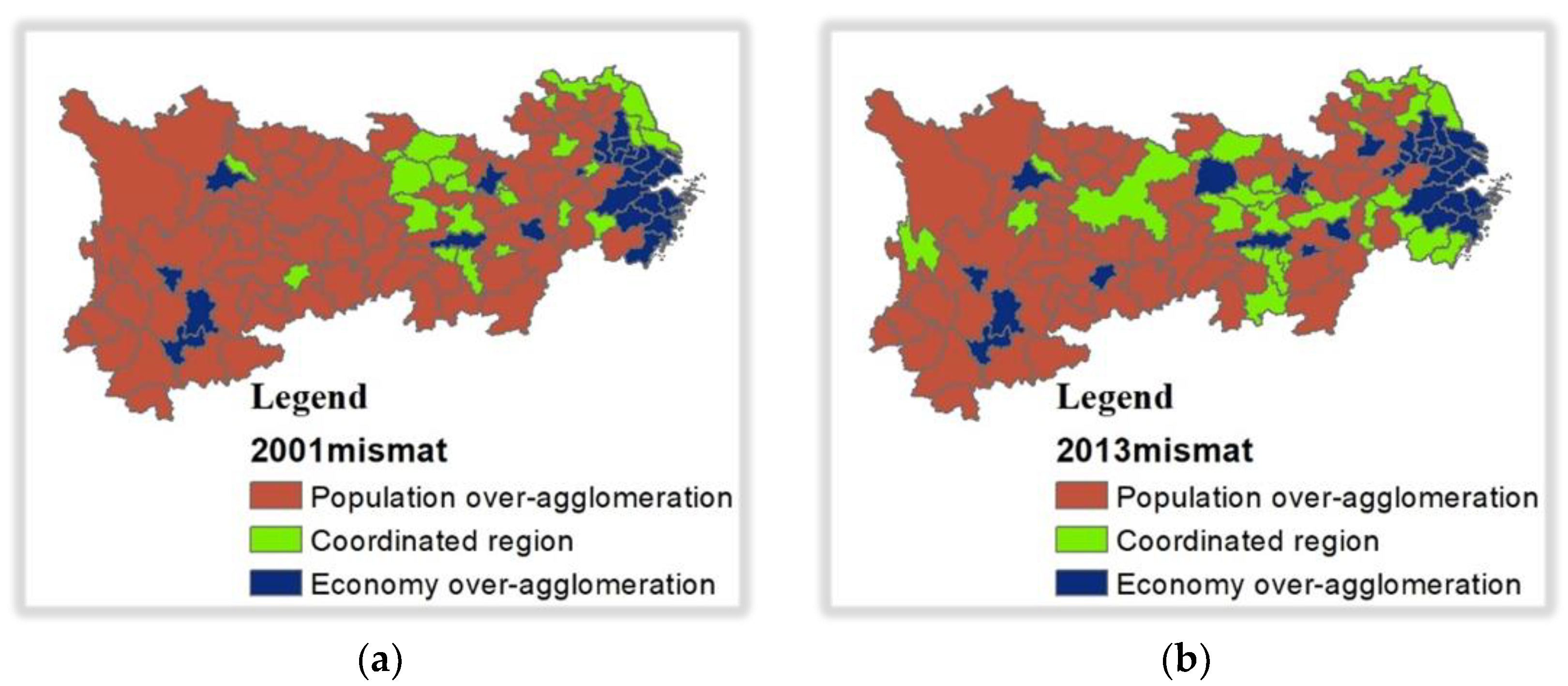
Based on the numerical values of CPE index, areas can be divided into three categories, this division is in line with the general practice and is consistent with the division by scholars who used the index (for example, [11,26]). The first category includes areas where the distributions of population and economy are basically consistent, which means that the population and economic distribution are relatively balanced (i.e., 0. 75 ≤ CPE ≤ 1. 25). The second category includes areas with the levels of agglomeration of the population higher than those of the economic agglomeration. In other words, the population is over-agglomerated (CPE < 0.75). The third category includes areas where the levels of economic agglomeration are higher than those of the population agglomeration. This would indicate that economic development is too agglomerated (CPE > 1.25).
Figure 2a shows the distribution of regional CPE values in YREB in 2001, Figure 2b shows the distribution of CPE in YREB in 2013. It can be seen that there are high CPE values in capital cities of all provinces in YREB. Comparing the two figures, the inconsistency between population and economic distribution changed only slightly with similar overall patterns over the 13-year period. The most obvious differences are in the central part of the YREB. There are more areas in the central area where population distribution and economic development are coordinated.

3.3. Determinants of CPE

Nowhere can a perfectly spatial consistency between population distribution and economic development be found in the world. The inconsistency is a ubiquitous phenomenon in economic geography. The New Geo-Economics [3,4,5,6,7,8,9,10] explains that economic gathering of goods and services determines how population and capital flow spatially. These flow processes themselves tend to continuously self-strengthen. This often results in different industries concentrating to different degrees on the inflows of population and capitals in a mechanism of causal circulation that gradually formed over time.
Williamson indicated that regional differences among regions in a country often showed a U-shape trend of changes against the improvement of economic development level, i.e., regional differences typically decline first, but they then rise after reaching the bottom of the trend against economic development. The internal mechanism for this trend is that, in the early stage of a region’s economic development, the polarization effect is likely to be greater than the trickling down (diffusion) effect in economically developed areas. Capital and labor flow from areas of lagging economies (backward areas) to developed areas. Local governments could adopt preferential policies to strengthen the economic development of developed areas for the higher marginal returns to the investment. However, this could cause the regional disparity in economic development to be enlarged. When a region’s economy develops to a certain stage where the growth pole becomes congested, and the marginal return to additional investment is diminishing, the government would likely gather sufficient financial resources to provide financial support to the backward areas. The developed areas form diseconomies of scale, which cause capital and labor to flow to backward areas, thus forming one or more secondary core areas in backward areas, thereby reducing the economic gap between regions.
Based on New Geo-Economics and related research [27,28,29,30,31,32,33], we can also understand the spatial inconsistency of population distribution and economic development from the perspective of resource allocation. In regional economic development, the dominant powers over the allocation of resources include market mechanism and government mechanism. On the one hand, according to the law of value, the resource allocation under the market mechanism is the most efficient, making the strong stronger and the weak weaker. This is also known as the wealth of the Matthew effect [34]. Hence, the market mechanism would allow capital and wealth to gather at a faster rate in the dominant area than the speed of population agglomeration.
On the other hand, a region’s population is also a production factor. When the market mechanism is in its full force, and there is no restriction to population movements, the population would be concentrated along with economic agglomerations. It should be noted, however, that changes in population distribution would respond to market mechanism slower than the changes in economic concentration would. Consequently, the role of the market mechanism leads to a bias in the distribution of population, which then causes the inconsistency between that and the region’s economic development.
Economic agglomeration is an inevitable trend of development, but excessive economic agglomeration may increase regional inequality, which may bring a series of problems to sustainable developments in some regions. To this end, local governments may consider formulating and implementing policy measures to influence population movements and guide capital flows at different stages of regional development to accelerate or mitigate the spatial inconsistency between population distribution and economic development. In that way, local governments can influence the consistency of the regional population and economic distribution.
According to the impact on the inconsistency by market mechanism, this study uses CPE index values as the dependent variable with the market functions and the government roles as explanatory variables to build an explanatory model. The independent, or explanatory, variables are described as follows: Where INVEST and SECEDU represent the roles of the market, TRANSP and POLICY represent the roles of the government, and INDSTRU and CPGDP are used as control variables.
INVEST denotes material capital of each region. It is the amount of investment of fixed assets to the GDP in the region. The fixed asset investment is a comprehensive indicator reflecting the scale, rate, proportion, and direction of the use of fixed assets. This is an expression for the physical capital status of regions under market influences. Data of INVEST is available from statistical yearbooks directly.
SECEDU denotes the human capital of each region. It is the number of people with completed secondary education per 10,000 people in each region. The reason why the number of people in secondary education in each region is used to represent human capital is that, it is difficult to get other indicators, and the current labor market has the largest proportion of people received secondary education.
TRANSP denotes the infrastructure in each region, which is the mileage of the highways inside each region. This indicator measures the accessibility and convenience of regional transportation systems and is an important part of public infrastructure construction. A good transportation infrastructure would reduce the human and material costs required for transportation and help to flow population and materials effectively. These, in turn, would have an impact on the population and economic distribution. Infrastructure construction is conducive to population movements and material flows. It promotes coordinated development of population and economic distribution.
POLICY is the regional policy, represented by per capita fiscal revenue and fiscal expenditure by regional governments. The effectiveness of regional policies depends on whether supporting funding is available. Usually, these funds are transferred to regions by the central government. It should be noted that the degree of bias of fiscal transfer payments to different regions is often reflected by the difference between fiscal revenue and fiscal expenditure. Therefore, this study uses per capita fiscal revenue and fiscal expenditure to reflect the impact of regional policy.
INDSTRU denotes the industrial structure in each region. This is expressed by the ratio of the GDP of the secondary industries and that of the tertiary industries. The influence of industrial structure on the spatial consistency of population distribution and economic development has two important components. First, the improvement of industrial structure would realize economies of scale and promote regional economic development. Second, the impact of industrial structure on employment structure would be largely affecting the movements of the population in the region. This study uses it as a control variable.
PCGDP denotes per capita GDP, which is an important indicator of region-wide macroeconomics and is used as a control variable in this study.
Data for human capital, infrastructure, regional policies, and per capita GDP, natural logarithmic processing was carried out before the econometrics analysis due to the varying numerical ranges of the data.

3.4. Research Method

Since economic phenomena usually have certain degrees of spatial agglomeration that can be detected and measured by calculating the level of spatial autocorrelation in the data, the spatial distribution of population and economic development should also be no exceptions. If this spatial dependency is overlooked, results from analyzing these distributions may lead to biased estimation of the consistency between them [35].
To overcome the shortcomings of traditional statistical analytical methods, spatial effects are considered in the analytical model in this study. Fully considering the influence of spatial dependence and spatial heterogeneity while constructing a generalized nested spatial panel data model [36,37], a spatial regression model is proposed as shown in the equation below.
y i t = α ι n + λ J = 1 N W i j y i j + β x i t + J = 1 N θ W i j x i j t + c i + ρ t + v i t v i t = η W v i t + ε i t
where
  • y denotes CPE, ι n is a unit vector of N × 1 order, which is related to the estimated constant term α ;
  • W is an n-order spatial weight matrix, which reflects the dependence between regions (In the spatial econometric analysis, a spatial weight matrix is needed to express the spatial relationships among analyzed regions. Because the principle of spatial weight matrix is based on the concept of proximity, the weights are simple to construct. In the actual spatial econometric analysis, the spatial weight matrix as determined by this method has been widely used. Therefore, this paper sets the spatial weight matrix to a matrix of binary adjacency weights. That is, if the two regions are geographically bordered, the weight is set to 1, otherwise it is set to 0.)
  • W y is the spatial lag dependent variable, that is the endogenous interaction effect between n regions;
  • λ is a parameter reflecting the magnitude of this effect; similarly;
  • W x is the exogenous interaction effect of each independent variable;
  • θ is the parameter reflecting the magnitude of this effect;
  • β is the regression coefficient, and the explanatory variable X represents the determinants of CPE;
  • v i t is a random disturbance term;
  • c i is a spatial individual effect, reflecting individual regions do not change with time;
  • ρ t is a spatial time effect, reflecting all individual regions change with time.
Among these model parameters, the individual spatial effect and the temporal effect can be coded as dummy variables introduced to each spatial unit and temporal unit. The latter part of the equation represents the spatial interactions between random perturbation terms, and η is the spatial autocorrelation coefficient representing the magnitude of this effect.
This model can be decomposed into three different models. When θ = 0 , η = 0 , the model can be reduced to a spatial lag model, or a spatial autoregressive model. When λ = 0 ,   θ = 0 , it can be simplified to a spatial error model. When η = 0 , it would be simplified to a spatial Durbin model.
LeSage and Pace [38] and Elhorst [37] have both commented on whether there can be spatial spillover effects measurable by empirically setting point estimates (λ, θ, or η) in spatial regression models. To that end, they proposed some improvement measures. Specifically, the spatial spillover effect can be decomposed into a direct effect and an indirect effect, wherein the direct effect is the influence of the changes in an explanatory variable in the specific unit on the interpreted variable, and the indirect effect is the influence of the explanatory variable on the interpreted variable in other units.
Equation (2) can be re-written to a generalized spatial panel data model, as represented by Equation (3) below:
Y = I δ W 1 X β + W X θ + R
where R includes the error term and the intercept term, and the kth explanatory variable X from unit 1 to unit n, the partial derivative matrix of the corresponding Y expected value can be written as Equation (4).
[ EY x 1 k · EY x N k ] = [ E y 1 x 1 k · E y 1 x N k · · · E y N x 1 k · E y N x N k ] = I δ W 1 [ β k w 12 θ k · w 21 θ k β k · · · · w 1 N θ k w 2 N θ k · w N 1 θ k w N 2 θ k · β k ]
where β k is the interpretation coefficient of the kth explanatory variable to the interpreted (dependent) variable. Each main diagonal element in the matrix represents a direct effect. The remaining elements are indirect effects. If δ = 0 and θ k = 0, then all non-diagonal elements would all become zero and indirect effects would not occur.

4. Model Results and Analysis

4.1. Tests of Spatial Dependency

Before the empirical analysis of the spatial regression models, the spatial autocorrelation test was performed on the variables from 2001 to 2013 to verify whether there exists any statistical significance of spatial autocorrelation in any of the variables. It can be seen in Table 1 that all indicators show some levels of statistical significance in terms of spatial agglomeration as measured by the positive values of calculated Moran’s Index. This result suggests that the study of the spatial consistency of population distribution and economic development in the 2001–2013 YREB could proceed with using panel data analysis with spatial effects.

4.2. Model Selection

In order to select the most suitable panel model with spatial effects, this study first carried out a series of tests. The city-level data of YREB was collected for the duration from 2001 to 2013. The study period (denoted as T) spans over 13 years. The spatial extent of the study area (namely N) includes 128 regions in YREB. With N being much greater than T, the unit root and cointegration test are not needed before the panel econometrics regression.
First, the significance test of Lagrangian multiplier statistical index (LM-Error and LM-Lag) was performed to determine the selected spatial effect model. The results are shown in Table 2. According to Anselin’s discriminant rule [39], both the LM-Error and LM-Lag indicators for our model passed the significance test, i.e., the Robust LM-Error indicator passes the significance test and the Robust LM-Lag indicator does not pass the significance test. Therefore, the spatial error model should be selected as the final form of the panel regression model.
As this study examines the spatial inconsistency problem between population distribution and economic development, the spatial lag model is more suitable for explaining the economic problems (such as economic growth) than the spatial error model would be. Therefore, even if the statistics of the spatial lag model are relatively smaller than that of the spatial error model, and as long as the former is still significant, it was more appropriate in selecting the spatial lag model as the final regression form than other forms because of the explanation power.
At the same time, when choosing which model to apply, one must consider the spatial effects of the dependent variable and the independent variables simultaneously. Therefore, the spatial Durbin model suggested by Elhorst [40] was chosen. The Durbin model can be a general form for the spatial regression model. If needed, the Wald test or log-likelihood ratio test can be used to determine whether the spatial Durbin model can be reduced to a spatial lag model or a spatial error model.
Based on the results of the likelihood ratio (LR) test, the spatial effect test had an estimated value of 1758.662 with the degree of freedom of 128 and a significance value (p) that was less than 0.01. The null hypothesis of no statistical significance must be rejected. Similarly, the time effect test had an estimated value of 614.872 with a degree of freedom of 13 and a significance value p that was less than 0.01. Again, the null hypothesis must be rejected. Therefore, the model should be extended to a model such that it would have both spatial fixed effects and time fixed effects. Consequently, the model is a two-way fixed effect model [41].
In addition, since the Durbin model includes both endogenous interaction effects and exogenous interaction effects, it is theoretically stronger than a simple spatial lag model or a simple spatial error model. For building the model, Matlab software was used to perform spatial Durbin model testing to determine whether the spatial Durbin model could be reduced to a spatial lag model or a spatial error model.
According to the p values of the Wald and LM statistic tests, the results show that the p values were less than 0.05, the original hypothesis was rejected, and the final regression form could not be reduced to a spatial error model or a spatial lag model.
Finally, we can choose for the model whether to include a fixed effect or a random effect, based on whether the error term of the panel data model is related to the independent variables. There are two types of error terms here, one is only related to the cross-section individual regions that would not change with time while the other is the unobservable factors that would change with time. The rule for the selection is to see if the latter is related to the independent variables. If it is relevant, one would choose a model with a fixed effect. Otherwise, a model with a random effect should be selected.
The decision method used the Hausman test [40]. The Matlab software was used to perform the Hausman test on the spatial Durbin model. Results were the t value being 85.765, the degree of freedom being 13, and the p-value being 0.000. Since the p-value was less than 0.025, the null hypothesis was rejected, and the fixed effect was selected.
In the end, in combination with the above test results, a Durbin model with two-way fixed effect was constructed. Given this selection and, according to Anselin’s research, the maximum likelihood method (ML) was used to estimate the parameter values of the spatial panel model [39].

4.3. Results of Regression Analysis

Through a series of tests, including a significance test of the Lagrangian multiplier statistical indicators (LM-Error and LM-Lag), a likelihood ratio (LR) test, and a spatial Durbin model test, the most suitable final regression model of this study was a two-way fixed effect Durbin model. In order to verify this result and compare it with other possible forms, the spatial lag model and the spatial Durbin model with four different effects that are not fixed effect, spatial fixed effect, time fixed effect and two-way fixed effect are compared.
Based on the levels of the goodness-of-fit, the spatial lag model with two-way fixed effect and the spatial Durbin model with two-way fixed effect have the best fit. This is consistent with the test results. Considering the value of log-L, two-way fixed effect model and bias-corrected two-way fixed effect model should be chosen. Because the bias-corrected two-way fixed effect model would avoid biased estimates of (some of) the parameters [37], we used the analysis results of the bias-corrected two-way fixed effect model to perform subsequent analysis. Table 3 shows the results.
The lag term W*dep.var (This denotes the spatial lag term of the dependent variable.) of the dependent variables in the three models did not pass the significance test, indicating that CPE values had no spatial aggregation and would not be affected by adjacent regions. This result may be due to exogenous interaction effects. Based on the results from the modified two-way fixed effect spatial Durbin model, the independent variables had passed the 1% significance test except for the infrastructure variables (TRANSP). The human capital (SECEDU) and regional policy variables (POLICY) had negative signs. This indicates that it had a negative effect on CPE values, and the sign of the material capital variable (INVEST) was positive, indicating that it had a positive effect on CPE values.

4.4. Spillover Effect Analysis

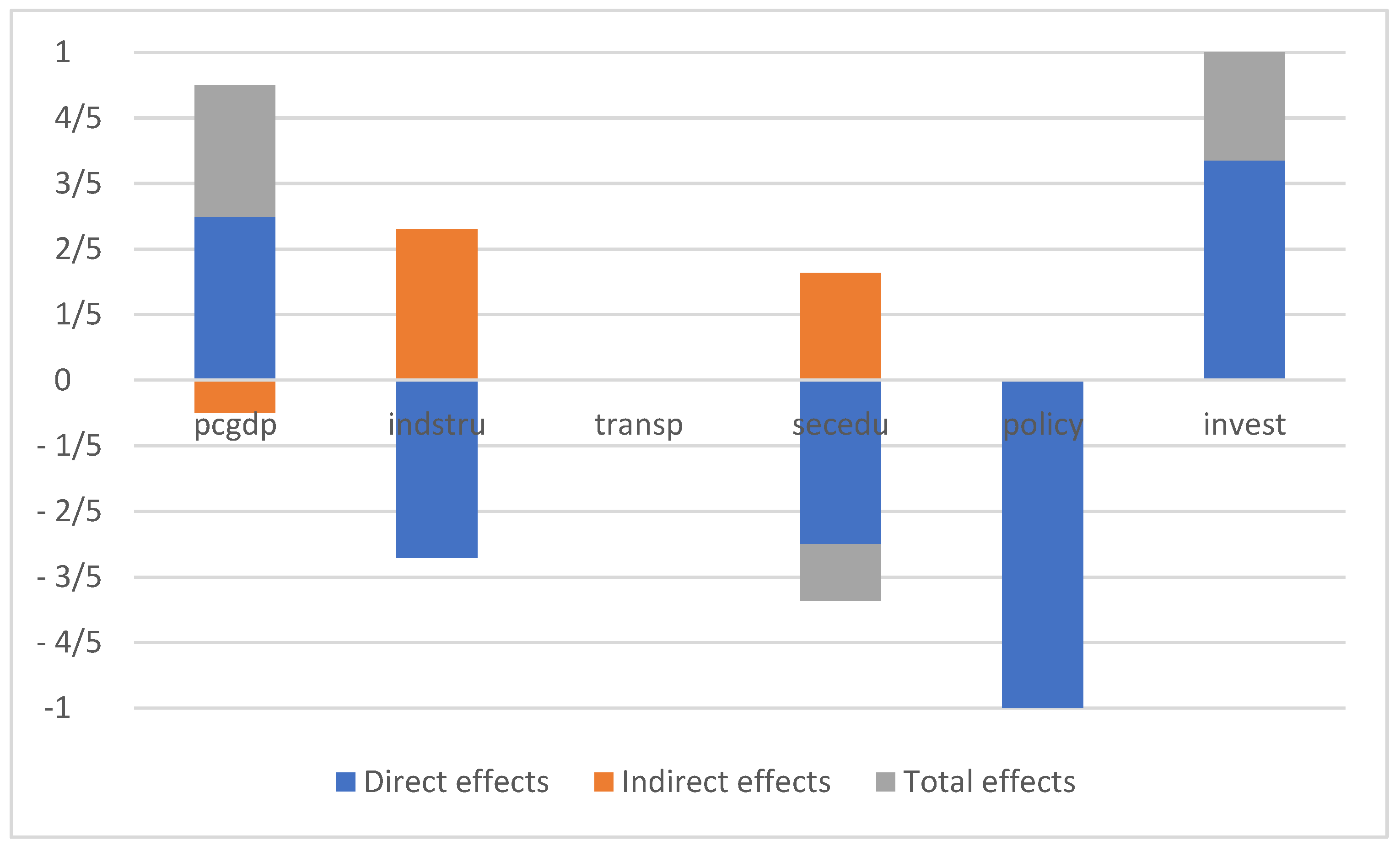
The direct effect, the indirect effect, and the total effect were calculated and the influence of the independent variable on the dependent variable was obtained. According to the recommendations by LeSage and Pace [38], the direct effect here reflected the average influence of a certain independent variable in a region on the dependent variable of the region, the indirect effect here reflected the influence of an independent variable in a region on the dependent variable of the adjacent region, and the total effect reflected the influence of an independent variable on the overall dependent variable, which could be calculated from the sum of the direct and indirect effects. For the model in this study, the direct and indirect effects of the error-corrected two-way fixed-space Durbin model were calculated and shown in Figure 3.
The direct effect here is different from the regression coefficient of the explanatory variable in Table 3. This is the elasticity after the feedback effect (transmitted through the adjacent region and transmitted back to the region). The elasticity of the variable of physical capital (INVEST) was 0.163, and the elasticity of the variable of human capital (SECEDU) was −0.282. This means that increasing the input of material capital had a positive impact on CPE and that increasing the input of human capital had a negative impact on CPE values. The infrastructure investment variable had no significant impact on CPE values. The elasticity of the variable of regional policy (POLICY) was −0.099, which indicated that the formulation and implementation of regional policies had a negative impact on CPE values.
The indirect effect estimate represents the spatial spillover effect of the variable. It can be seen from the results that the increase in per capita GDP positively affected CPE of the region, but negatively affected CPE values of the adjacent regions. In contrast, the increase in human capital and the optimization of the industrial structure had a negative impact on CPE value of the region, while positive impacted on the adjacent region. However, the spatial spillover effects of regional policies, physical capital, and infrastructure on CPE values were not significant.
In terms of the total effect, the impact of infrastructure (TRANSP) on CPE values was still not significant. The change in the industrial structure had no significant effect on CPE value because the industrial structure had the opposite direction of influence on CPE value of the region and one of the adjacent regions. Overall, it was not clear which region had been impacted more than others. The input of human capital had a negative impact on CPE value. This effect was mainly due to its direct effect. The increases in physical capital investment and per capita GDP had positive impacts on CPE. This effect was mainly due to their direct effects.

5. Conclusions

Motivated by the existing inconsistency between population and economic distributions in YREB, this paper used a two-way fixed space Durbin model to analyze the factors affecting the coordination of population–economic distributions in YREB. This study also further analyzed the direct effects and indirect effects of various factors affecting population–economic coordination.
The research results are as follows.
(1)
The economic development is too spatially agglomerated in and around provincial capital cities in YREB. The population is over-agglomerated in other cities of all provinces in YREB. The results suggest the need to further strengthen the flows of population or to strengthen the economic development of small towns such as counties and towns.
(2)
From the perspective of the total effect, different factors have shown to have different effects on the degrees of population–economic coordination in YREB. Infrastructure changes have no significant impact on CPE values. Human capital has a negative impact on CPE values. Physical capital and per capita GDP have a positive impact on CPE values.
(3)
The increase in human capital has a negative impact on CPE values, but the spillover effect from core areas to adjacent areas is positive, indicating that the increase of human capital has a greater impact on core regions than on their adjacent areas. The industrial structure has the opposite direction of influence on CPE values between the region and the adjacent region. It should be noted that it is still difficult to judge which region has more effect on the imbalance of the population–economic coordination as a whole.
(4)
The spillover effect of per capita GDP increase is significantly negative, and the spillover effect of the human capital increase and industrial structure optimization are significantly positive. In addition, the spatial spillover effects of regional policies, physical capital, and infrastructure on CPE values are not significant.
Since the CPE value is optimal within a threshold range (i.e., 0.75 < CPE < 1.25), a value higher than 1.25 represents an excessive agglomeration of the economy and a value lower than 0.75 represents an over-aggregation of the population. In this paper, we framed the positive impacts as promoting economic agglomeration and the negative impact as promoting population agglomeration. Therefore, regardless of the roles that the market or the governments play in promoting coordinated development of population distribution and regional economy, the magnitude of the force is difficult to grasp or defined precisely.
The discussion in this paper shows that the improvement of human capital and the tilt of regional policies are conducive to population agglomeration. Alternatively, increasing the input of physical capital can promote economic agglomeration. From the spatial econometric analysis carried out in this study, the direct and indirect effects often have opposite directions. Therefore, it is necessary to consider indirect effects when governments implement policies or intervention programs.
Most of the population and economic high-value distribution areas are located in capital cities in 2013, and it can be inferred that most of the regions of YREB are in a polarized stage. From the coordinated distribution of population distribution and economic development in 2001 and 2013, the economic development of coastal areas is in the stage of both polarization and diffusion. Therefore, different regions of YREB are at different stages of inverted U-shaped economic development. The government’s tilting policy needs to take into account different developed regions and different backward regions. How does the government regulate and narrow the regional gap from a macro perspective? Based on the theoretical analysis and the empirical analysis of this paper, it is suggested that (1) relevant policies can be further tuned to allow free and full flows of floating population so to effectively reflect market mechanism, (2) avoid omitting the needs for public support in developed regions when the government begins or aggressively starts investing in the backward regions, and (3) for backward regions, it is necessary to let market mechanism guide governmental investments through public policies and intervention programs.
For a better understanding of the situation, it would be interesting to identify the relationship between the development of certain industries and the influx of people into the region. Understanding of this relationship could help macroeconomic management.

Author Contributions

H.X. organized this study and conducted study design, performed the econometrics analysis and revision of the manuscript; J.Y. contributed to interpretation of analysis, and revision of the manuscript; X.L. contributed to prepared datasets, performed the statistical analysis and drafted the manuscript; J.L. contributed to interpretation of analysis, and revision of the manuscript, modifying and polishing written English.

Funding

This study was financially supported by National Social Science Fund of China (No. 18ZDA132) and the Ministry of Education of the People’s Republic of China (No. 17JHQ041).

Conflicts of Interest

The authors declare no conflict of interest.

References

  1. Williamson, J.G. Regional inequality and the process of national development: A description of the patterns. Econ. Dev. Cult. Chang. 1965, 13, 1–84. [Google Scholar] [CrossRef]
  2. Kuznets, S. Economic Growth and Income Inequality. Am. Econ. Rev. 1955, 45, 1–28. [Google Scholar]
  3. Krugman, P. Geography and Trade; Leuven University Press: Leuven, Belgium, 1991. [Google Scholar]
  4. Krugman, P. Development, Geography and Economic Theory; MIT Press: Cambridge, MA, USA, 1995. [Google Scholar]
  5. Fujita, M.; Krugman, P. The new economic geography: Past, present and the future. Pap. Reg. Sci. 2004, 83, 139–164. [Google Scholar] [CrossRef]
  6. Krugman, P. The new economic geography, now middle-aged. Reg. Stud. 2010, 45, 1–7. [Google Scholar] [CrossRef]
  7. Fingleton, B.; Fischer, M.M. Neoclassical theory versus new economic geography: Competing explanations of cross-regional variation in economic development. Ann. Reg. Sci. 2010, 44, 467–491. [Google Scholar] [CrossRef]
  8. Redding, S.J. Economic geography: A review of the theoretical and empirical literature. In Palgrave Handbook of International Trade; Springer: Berlin, Germany, 2013; pp. 497–531. [Google Scholar]
  9. Ghiglino, C.; Nocco, A. When Veblen meets Krugman: Social network and city dynamics. Econ. Theory 2017, 63, 431–470. [Google Scholar] [CrossRef]
  10. Gaspar, J.M. A prospective review on New Economic Geography. Ann. Reg. Sci. 2018, 6, 237–272. [Google Scholar] [CrossRef]
  11. Feng, Z.; Liu, X. Research on Spatial Consistency of Population Distribution and Economic Development in China. Popul. Econ. 2013, 2, 3–11. [Google Scholar]
  12. Xiao, Z. A Study on the Spatial Effect of the Consistency of Population and Economic Distribution in China. Popul. Res. 2013, 37, 42–52. [Google Scholar]
  13. Soltani, S.R.; Mahiny, A.S.; Monavari, S.M.; Alesheikh, A.A. Sustainability through uncertainty management in urban land suitability assessment. Environ. Eng. Sci. 2013, 4, 170–178. [Google Scholar] [CrossRef]
  14. Yang, C.; Han, H.; Song, J. Spatial Distribution of Migration and Economic Development: A Case Study of Sichuan Province, China. Sustainability 2014, 6, 6509–6528. [Google Scholar] [CrossRef] [Green Version]
  15. Yang, Q.; He, L. Spatiotemporal changes in population distribution and socioeconomic development in China from 1950 to 2010. Abrab. J. Geosci. 2017, 10, 498. [Google Scholar] [CrossRef]
  16. Paul, S.; Chatterjee, K. Urbanisation and consistency measurement: A study on District of North 24 Parganas, West Bengal, India. Arch. Appl. Sci. Res. 2012, 4, 2052–2067. [Google Scholar]
  17. Souche, S.; Mercier, A.; Ovtracht, N. The impacts of urban pricing on social and spatial inequalities: The case study of Lyon (France). Urban Stud. 2016, 53, 373–399. [Google Scholar] [CrossRef]
  18. Song, S.; Chu, G.S.F.; Chao, R. Inter-city regional disparity in China. China Econ. Rev. 2000, 11, 246–261. [Google Scholar] [CrossRef]
  19. Golley, J.; Wei, Z. Population dynamics and economic growth in China. China Econ. Rev. 2015, 35, 15–32. [Google Scholar] [CrossRef]
  20. National Sanitation and Health Commission of China. China’s Floating Population Development Report 2018; China Population Publishing House: Beijing, China, 2019.
  21. Francis, J. Asymmetries in regional labor markets, migration and economic geography. Ann. Reg. Sci. 2007, 41, 125–143. [Google Scholar] [CrossRef]
  22. Perroux, F. Economic Space: Theory and Applications. Q. J. Econ. 1950, 64, 89–104. [Google Scholar] [CrossRef]
  23. Hoover, E.M.; Giarratani, F. An Introduction to Regional Economics, 3rd ed.; Mcgraw-Hill: New York, NY, USA, 1999. [Google Scholar]
  24. Nijkamp, P.; Abreu, M. Regional Development Theory. In International Encyclopedia of Human Geography; Kitchin, R., Thrift, N., Eds.; Elsevier: Amsterdam, The Netherlands, 2009; Volume 9, pp. 202–207. [Google Scholar]
  25. Martin, R.; Sunley, P. The new economic geography and policy relevance. J. Econ. Geogr. 2010, 11, 357–369. [Google Scholar] [CrossRef]
  26. Zhang, J.; Guo, X. A Theory and Empirical Model of Long-term Balanced Population Development. Popul. Res. 2013, 37, 16–29. [Google Scholar]
  27. Hoover, E.M. Basic Approaches to the Study of Demographic Aspects of Economic Development: Economic-Demographic Models. Popul. Index 1971, 37, 66–75. [Google Scholar] [CrossRef] [PubMed]
  28. Niebuhr, A. Market access and regional disparities. Ann. Reg. Sci. 2006, 40, 313–334. [Google Scholar] [CrossRef]
  29. Egger, P.; Gruber, S.; Larch, M.; Pfaffermayr, M. Knowledge-capital meets new economic geography. Ann. Reg. Sci. 2007, 41, 857–875. [Google Scholar] [CrossRef]
  30. Ter Wal, A.L.; Boschma, R.A. Applying social network analysis in economic geography: Framing some key analytic issues. Ann. Reg. Sci. 2009, 43, 739–756. [Google Scholar] [CrossRef]
  31. Mossay, P. A theory of rational spatial agglomerations. Reg. Sci. Urban Econ. 2013, 43, 385–394. [Google Scholar] [CrossRef]
  32. Pessoa, A. Agglomeration and regional growth policy: Externalities versus comparative advantages. Ann. Reg. Sci. 2014, 53, 1–27. [Google Scholar] [CrossRef]
  33. Barbero, J.; Zofío, J.L. The multiregional core-periphery model: The role of the spatial topology. Netw. Spat. Econ. 2016, 16, 469–496. [Google Scholar] [CrossRef]
  34. Merton, R.K. The Matthew Effect in Science. Science 1968, 159, 56–63. [Google Scholar] [CrossRef]
  35. Ji, M.; Wu, Z.; Su, H.; Jiang, L. Spatial Panel Analysis of China’s Economic Growth and Institutional Change. Areal Res. Dev. 2011, 30, 1–5. [Google Scholar]
  36. Ge, Y. How does urbanization in China affect fertility? Based on the study of spatial panel data model. Popul. J. 2015, 37, 88–101. [Google Scholar]
  37. Elhorst, J.P. Matlab Software for Spatial Panels. Int. Reg. Sci. Rev. 2014, 37, 389–405. [Google Scholar] [CrossRef]
  38. LeSage, J.P.; Pace, R.K. Introduction to Spatial Econometrics; CRC Press Taylor & Francis Group: Boca Raton, FL, USA, 2009. [Google Scholar]
  39. Anselin, L. Spatial Econometric: Methods and Models; Kluwer Academic Publishers: Dordrecht, The Netherlands, 1988. [Google Scholar]
  40. Elhorst, J.P. Spatial Panel Data Models; Springer: Heidelberg, Germany, 2010. [Google Scholar]
  41. Baltagi, B.H.; Song, S.H.; Jung, B.C.; Kon, W. Testing for serial correlation, spatial autocorrelation and random effects using panel data. J. Econom. 2007, 140, 5–51. [Google Scholar] [CrossRef]
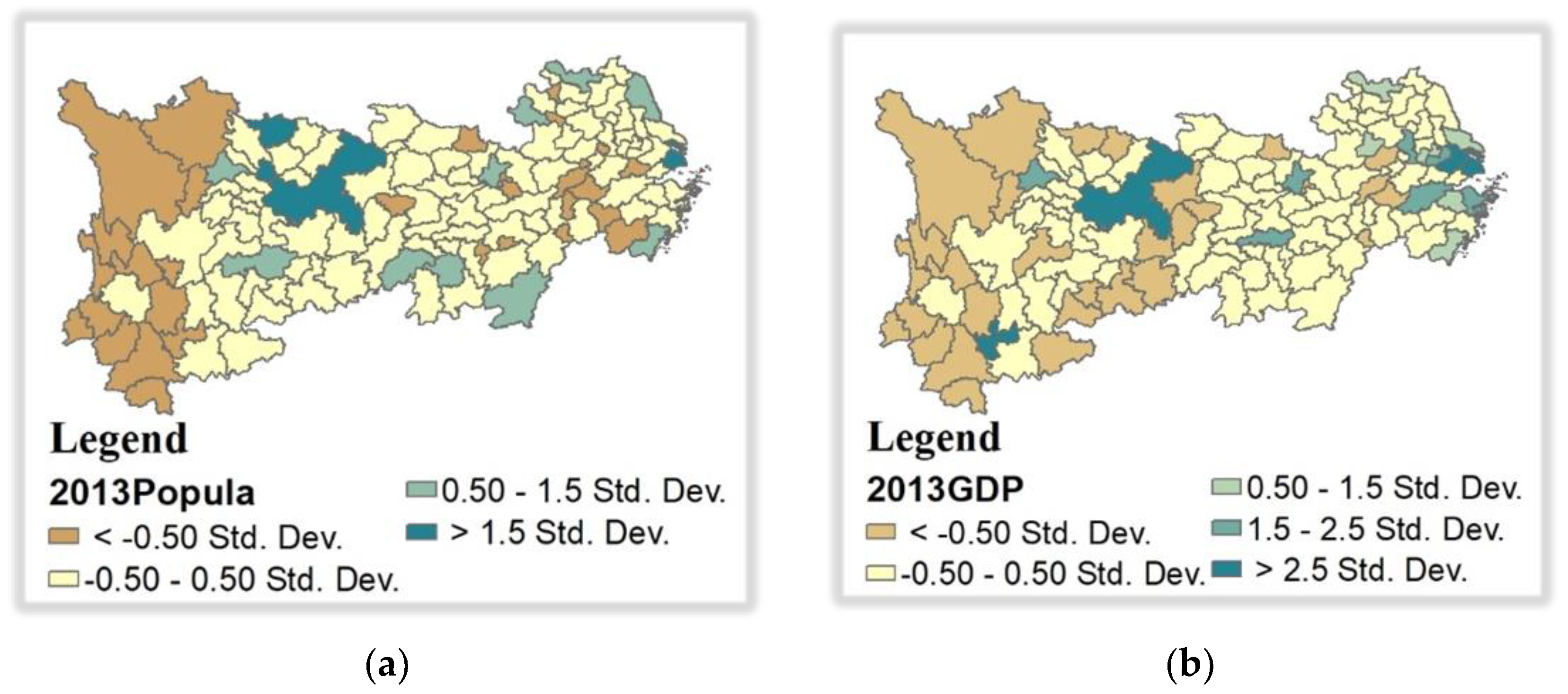
Figure 1. (a) Distribution of population in YREB. (b) Distribution of economic product in YREB.
Sustainability 11 03320 g001
Figure 2. (a) CPE values in YREB, 2001. (b) CPE values in YREB, 2013.
Sustainability 11 03320 g002
Figure 3. The direct effect, indirect effect, and total effect of spatial Durbin model with two-way fixed effect.
Sustainability 11 03320 g003
Table 1. Global Moran’s I of variables from 2001 to 2013.
YearCPEINVESTSECEDUTRANSPPOLICYINDSTRUPCGDP
20010.533 ***0.196 ***0.492 ***0.215 ***0.426 ***0.218 ***0.544 ***
20020.545 ***0.295 ***0.625 ***0.171 **0.415 ***0.204 ***0.549 ***
20030.558 ***0.296 ***0.678 ***0.157 **0.435 ***0.211 ***0.556 ***
20040.564 ***0.305 ***0.600 ***0.162 **0.445 ***0.170 **0.555 ***
20050.531 ***0.235 ***0.605 ***0.151 **0.395 ***0.204 ***0.524 ***
20060.504 ***0.236 ***0.550 ***0.097 *0.421 ***0.123 *0.483 ***
20070.531 ***0.269 ***0.482 ***0.105 *0.443 ***0.102 *0.511 ***
20080.514 ***0.213 ***0.416 ***0.102 *0.423 ***0.137 **0.493 ***
20090.502 ***0.367 ***0.289 ***0.126 *0.417 ***0.190 ***0.488 ***
20100.497 ***0.361 ***0.387 ***0.159 **0.273 ***0.236 ***0.487 ***
20110.485 ***0.337 ***0.475 ***0.145 **0.386 ***0.278 ***0.478 ***
20120.440 ***0.339 ***0.503 ***0.142 **0.331 ***0.299 ***0.442 ***
20130.147 ***0.154 **0.182 ***0.126 *0.207 ***0.317 ***0.347 ***
Note: *, **, and *** represent the significance levels of 10%, 5%, 1% respectively. The spatial weight matrix (W) used here is constructed based on the contiguity relationship.
Table 2. The test results of spatial correlation.
Statistic of TestPooled OLSSpatial Fixed EffectsTime-Period Fixed EffectsSpatial and Time-Period Fixed Effects
LMlag182.3400.15443.0020.866
(0.000)(0.695)(0.000)(0.352)
R_LMlag0.76376.45711.9028.809
(0.382)(0.000)(0.001)(0.003)
LMerr438.45415.46650.7910.714
(0.000)(0.000)(0.000)(0.398)
R_LMerr256.87791.76919.6918.657
(0.000)(0.000)(0.000)(0.003)
Note: The model used is based on the Elhorst LM test, and the result is returned by the Matlab program code (www.regroningen.nl/elhorst), and p values is in parentheses.
Table 3. Regression results of spatial panel model.
DeterminantsRegression Coefficients DeterminantsRegression Coefficients
pcgdp1.633 ***W*pcgdp−0.373 ***
(33.713)(−3.337)
indstru−0.146 ***W*indstru0.124 **
(−4.407)(2.477)
transp−0.01W*transp0.001
(−0.332)(0.033)
secedu−0.283 ***W*secedu0.189 ***
(−7.860)(3.296)
policy−0.100 ***W*policy0.04
(−4.274)(0.924)
invest0.166 ***W*invest−0.086
(5.558)(−1.396)
W*dep.var0.033
(0.897)
R20.936
sigma20.05
log-L200.463
Note: t-values are in parentheses. *, **, *** represent the significance level of 10%, 5%, 1% respectively.