Evaluating Impacts of Overweight in Road Freight Transportation: A Case Study in Brazil with System Dynamics

Abstract

Overweight vehicles in ornamental stone transportation reduce the lifespan of the pavement and increase accidents on Brazilian highways. This paper evaluates the relationship between different policies for the loading of ornamental stone vehicles and its externalities, such as the impact on costs with transportation, pavement maintenance and road accidents, using the System Dynamics (SD) method. The results confirm the advantages of reducing operational costs with the practice of overweight. However, as the overweight increases, the pavement maintenance and road accidents costs also increase. Therefore, the best vehicle loading policy depends on the relative importance of the economic and social costs involved.

1. Introduction

The sustainable growth of a nation depends on efficient transportation systems. Many authors describe the positive relationship between the economic development of a country and its transportation infrastructure [1,2,3,4]. The public investment in transportation infrastructure causes a positive effect on long-term economic performance [5].

Brazil has difficulties in its road infrastructure that are caused by the imbalance between use and investments, which affects the country in rankings such as logistics performance, as published by the World Bank. In the edition of 2018, Brazil ranked 56th overall and 51st in the category of Infrastructure [6]. Still, in this category, the country ranked 73rd among 137 countries assessed by the World Economic Forum, which considers infrastructure as one of the pillars for global competitiveness [7].

Nevertheless, if on one hand the wide offer of transportation infrastructure is beneficial for economic development, on the other hand the increased demand for trips led to traffic jams, pollution and accidents, the social costs of which are unevenly distributed throughout the society. Freight transportation policies, specifically, impact a country’s economy, society and environment [8]. National economic growth depends on the activity of freight transportation and its infrastructure enables and supports economic growth [1]. Regarding the social and environmental areas, however, many impacts may result from the development of infrastructure and of product transportation operations and these impacts must be taken into consideration in the strategic planning of this sector [9].

One of the main problems of road freight transportation is overweight vehicles, which leads to the poor conditions found on Brazilian highways, to a reduction in the life span of vehicles, to the increase in fuel consumption and to a higher risk of accidents. The consequences of these problems are perceived by the degradation of road infrastructure in terms of pavement, by the high operational cost of transportation and by the decreased quality of the service being provided. Furthermore, overweight has been identified as one of the main causes of accidents involving trucks in Brazil [10]. A particular example of this problem in Brazil is that of ornamental stones transportation in the state of Espírito Santo, due to the gravity of accidents caused by the tipping of trucks loaded with marble and granite blocks.

The interest in assessing the social costs and the externalities of transportation, especially road transportation, has grown due to the need of more effective policies to control the negative effects associated with the problem of overweight vehicle [11]. Despite all the existing legal regulation in Brazil, there is still a high number of overweight vehicles traveling. The National Department of Transportation Infrastructure (DNIT) showed that 77% of carrier vehicles traveled overweight and that 10% of excess load per axle may reduce the predicted life span of a pavement in up to 40% [12].

On the other hand, the instruments used to quantify the impacts of the externalities caused by transportation are not satisfactory and there are controversies regarding the relationship between transportation and its impacts and regarding the associated costs calculation [11]. The economic impacts of transportation in different categories are presented, among which the following stand out: road operational costs (energy and workforce expenses); infrastructure damage costs (road maintenance costs); congestion and scarcity costs (delay costs imposed on users due to traffic congestion); environmental costs (noise, water, soil and air pollution); and accident costs (material damage and product losses) [13].

Therefore, in face of the impact of excess weight measuring challenge in freight transportation, which affects road infrastructure, safety and additional consumption of resources to maintain traffic conditions in the transportation network, the objective of this article is to assess the relationship between excess weight in the road transportation of ornamental stones, the transportation operational costs and the social costs with road accidents and pavement maintenance, using a System Dynamics (SD) model.

Transportation systems are complex and, therefore, public and/or private authorities need to test, in simulation environments, the policies and actions before they are effectively implemented in the real world, which is open and dynamic. Thus, SD may be used to simulate complex systems involving feedbacks in which human judgment, experience and logic are combined [14].

The remainder of the paper is organized as follows. Section 2 presents a literature review with different approaches to the problem of overweight in road transportation, converging to models that used SD. Section 3 shows materials and methods, the SD model structure and testing. Section 4 presents a case study addressing the problem of ornamental stones transportation in the state of Espírito Santo and details the input parameters and the data gathering methodology. Section 5 describes the simulated scenarios and also presents the results. Finally, Section 6 presents the final considerations.

2. Literature Review

Overweight vehicles in road transportation lead not only to mechanical failures in the vehicles themselves but also greatly accelerates pavement deterioration. For that reason, legislation in many countries determines the limits for axle loading and vehicle gross weight, while public agencies try to enforce these limits through vehicle weighing and inspection. Trucks that exceed the legal loading limits increase the risk of traffic accidents and lead to unfair competition between transportation companies.

Many studies in the literature address and try to quantify the impact of this practice, its consequences and possible mitigation actions, such as the development of technologies to inspect overloading in a more efficient way. However, this fact involves many elements, which makes it difficult to find studies that comprehend all aspects.

The problem of overloading was critical in Africa [15], where the incentives to overloading were high and the levels of inspection are low. The author proposed load measurement via the direct installation of load sensors on the axles to help vehicle operators safely find the most economic load considering road conditions and legal limits. Furthermore, regulatory authorities would have a way of checking load per axle at any moment and place, without the need for a permanent structure.

The frequent weighing of trucks slows the supply chain down and increases operational costs, emphasizing the importance of using information and communication technologies to share information [16]. Since South African overweight control centers do not have electronic tracking, the lines generated at the centers force some vehicles, which may be overloaded, to find a way around the inspection, damaging the pavement and increasing road maintenance costs. Because of that, the use of a system to identify these vehicles through automatic number plate recognition cameras was proposed [17]. These vehicles are considered non-compliant and the level of punishment to be applied will have to be determined by the road agencies but the authors suggest that a maximum penalty must be applied to discourage this behavior and to generate additional funds for road maintenance.

Weigh-in-motion (WIM) technologies are another alternative, since they allow trucks to be weighed in traffic, without any interruption in the operations, which may contribute to a safer and more efficient operation of trucks, helps to reduce the number of overweight trucks, contributes to efficient police time use and may reduce traffic accidents [18].

In 2005, the Ministry of Transportation in Egypt issued new regulations to increase the legal loads per axle for trucks. An assessment of truck factors (TF) regarding the old and new regulations using real truck loads and traffic data was presented [19]. TF are used to determine the equivalent single axle load (ESAL) needed for projects and pavement maintenance, which increased with the expansion of allowed tolerance. This impact was converted into additional asphalt thickness, increasing the pavement maintenance costs.

The impact of the new axle load tolerance for vehicles in Egypt on pavement maintenance costs and operational costs of transportation using the HDM-4 were assessed [20]. Model under different levels of inspection, road maintenance options and different vehicle loading policies. The results showed that, although the increased load per axle requires a pavement of greater structural capability, the lower number of trips per truck required to transport the same load may lead to a reduction in the operational cost of transportation, thus causing the increase in load limit to be considered useful.

However, the costs considered [20] are not the only impacts caused by the practice of overloading and it is necessary to consider, for example, costs with road accidents, environmental impacts and trip time, the latter affecting all road users. Moreover, the agents responsible for each cost category are also different. Therefore, the managers responsible for regulation and inspection should prioritize the minimization of the most relevant costs according to the objectives of the established public policies.

Based on a case study of Mexico, a bi-level modeling approach was presented [21] to represent the interaction between the vehicle loading practices of carriers and the decisions made by road planning authorities, which are responsible both for maintenance and overload control. Results show that at a lower level (reactive), decisions made by carriers regarding overload impact road maintenance expenses, while at an upper level (preventive), the planner decides about inspection levels anticipating carrier responses.

Another method used in the literature to assess the systems behavior regarding load policies and excess weight in freight vehicles is System Dynamics (SD). The term system refers to a set of elements that interact with each other and the term dynamic refers to systems which variables are constantly changing over time. The system dynamics emphasized the multiloop, multistate, nonlinear character of the feedback systems. The existence of multiple interacting feedbacks means it is difficult to hold other aspects of the system constant to isolate the effect of the variable of interest. Therefore, SD is a method that studies the changes in the behavior of a system over time to assess impacts of decision making at a strategic level [22,23,24,25].

The system may be represented via two approaches: qualitative and quantitative [26,27]. The qualitative model is built on causal loop diagrams that represent the feedback relationships between the variables that define the model’s behavior [28]. In the quantitative approach, the system is detailed in the stock and flow diagram, configuring differential equations that are numerically solved by means of dynamic simulation (numerical integration). For more details about the SD method, the causal loop diagram, the stock and flow diagram and the model tests, please check [22,26,27,28,29,30,31,32].

In the context of road maintenance operations, a SD model was developed to simulate the impact of maintenance and obsolescence of a road system and to define the relationship between maintenance activities and traffic volume with the use of road revenue generated by traffic to maintain the pavement’s operation level [33]. Thus, the simulation model supports the decision about the best use of available resources.

A SD model for the simulation of road degradation and restoration processes was presented, calibrated with data from eight road sections in Virginia (USA) and coupled to an optimization module of maintenance operations whose approach provides a plan of best practices for road maintenance [34]. The results suggest that the shift to a less costly preventive maintenance, instead of a more expensive (and more time-consuming) corrective maintenance, should bring benefits to the system as a whole. However, the policy of preventive maintenance was questioned [35] and another model of the effect of road conditions on the index of road accidents was presented. With data from the region of New England (USA), it demonstrates that the mental model behind the policy of road improvement could, in most cases, increase accidents due to higher speeds and better pavement conditions. The author shows the consequences of the maximization of road repairs with resource expenses, which can be causing more accidents.

Nevertheless, the context in which the above-mentioned studies were carried out belongs to a road system with a developed infrastructure, in other words, with high capacity expressways whose management focuses only on maintaining good conditions of already existing trafficability. This reality, however, is not consistent with the conditions of a good part of the road network in developing countries, such as Brazil, according to studies indicated by the National Confederation of Transport [36].

In an emerging country such as China, a SD model was built to analyze the regulation of the weight of freight vehicles and to assess the impacts of their overloading [37]. According to the authors, such regulation has significant economic consequences, such as increase in the transportation cost per truck and reduction in the cost of construction, maintenance, convenience and safety of highways.

Another SD model was proposed to evaluate the long-term effects of weight regulation policies of trucks in China on the sustainability of the activity [38]. The model presents the cumulative economic cost, including the operational cost and the cost associated with transportation time, in addition to the accumulated social cost, including pavement maintenance, pollutant emissions and accident costs, so that the policy effects on road transportation sustainability could be evaluated.

The problem of vehicle overloading in China [38] is similar to the one found in freight transportation on Brazilian highways. However, the model presented by the authors has some limitations, such as the consideration of a route dedicated to transport a specific load. This means that traffic in the studied route is composed of only one type of vehicle and that there is no variability of traffic volume along the route. Such characteristics have an impact on important variables, such as road capacity, travel time and, consequently, operational cost of transportation.

In fact, the application of strict loading policies in China has not progressed well due to the increase in transportation costs and the reduction of the activity’s economic performance. Then, a SD model was developed to perform a long-term evaluation of the alternative modal shift policies, encouraging a greater use of more efficient modes of transportation, such as railways, with results showing that it was an effective option to achieve sustainability in the activity, reducing social, environmental and economic costs of freight transportation [39].

In short, with SD it is possible to understand and evaluate the behavior of the road freight transportation system with overloading and its impacts on other parameters, such as the economic and social costs involved. However, some gaps in the existing literature have been identified such as the lack of a model closer to the real operational conditions of Brazilian highways, with diversity in volume and categories of vehicles. Therefore, the literature has not provided models involving different vehicles with different load volumes traveling along the same route which could be applicable to Brazilian reality.

In Brazil, ornamental stones road transportation presents the problem of overload, which causes damage that are often not accounted for or considered in the strategic decisions of the sector. For that reason, the transportation of ornamental stones in the Brazilian southeast region was chosen as the object of a case study for the development of a SD simulation model that covers required characteristics, aiming to help in the development of more effective policies for sustainability in transportation.

3. Materials and Methods

Considering the limitations of the models in the literature regarding the application of SD to problems that involve overweight vehicles, this study proposed a model addressing the impacts of this practice on road transportation.

3.1. Model Structure

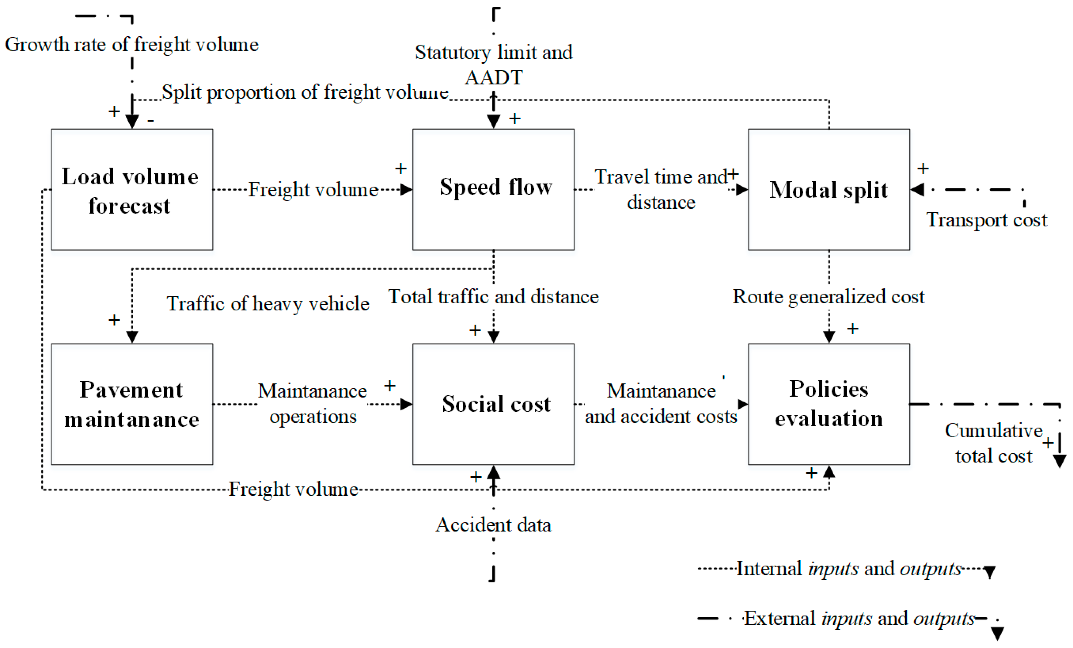
The variables in the model were grouped into six interrelated models, as shown in the causal loop diagram in Figure 1. To perform the simulation, each module of the model was structured into stock and flow diagrams presented in more details as follows.

The first module addresses “Load Volume Forecast,” shown in Figure 2. In this module, trips are caused by the production of a given product and are carried via the road mode. Different routes can be available to transport the load volume forecasted, that can be called Route #1 and Route #2, for example. The objective of the module “Load Volume Forecast” is, therefore, to calculate the volume of load, in tons, that will be transported via each considered route.

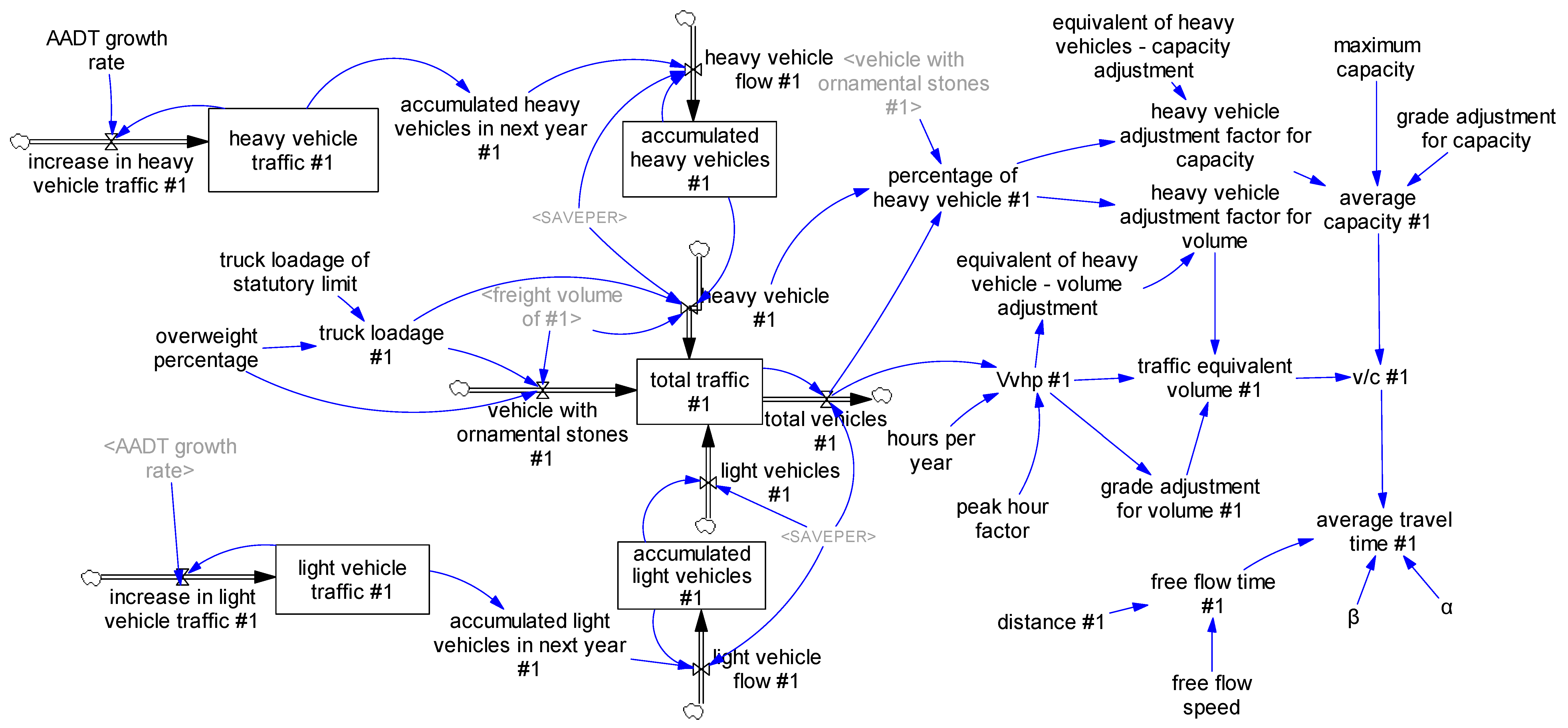
The module presented in Figure 3 regards “Speed Flow” and its objective is to provide the travel time in each road route. Due to the differences of each part of the road, called link, as the number of travelling vehicles and their speed, travel time is calculated separately and, at the end, added to the total transportation time of each road route. Figure 3 shows the structure of the simulation model for the travel time of a single link of a given route, which can be replicated to the number of links on the available routes.

The upper part of the diagram shows the traffic of the freight vehicles, called heavy vehicles, to differentiate them from those that are overloaded, in the middle part of the diagram. The lower part of the diagram shows the traffic of light vehicles.

Given the total volume of vehicles, it is necessary to convert it into unit of passenger car equivalent (PCE), defined by Highway Capacity Manual—HCM [40]. To calculate road capacity, HCM also provides the adjustment factors, due to the presence of heavy vehicles, which reduces the traffic speed of the highway. After finding out the load of the whole network, an analysis of each road link is carried out aiming to determine the relationship between equivalent traffic volume and the average capacity of the link. Equation (1) [41] is applied to find out the travel time spent in the analyzed road link.

$$t= t_0·(1+\alpha ·{\left(V/C\right)}^{\beta }$$

(1)

where:

• t: adjusted time in which volume V may use road link;
• t₀: travel time for a free flow condition;
• V: traffic equivalent volume;
• C: road capacity; and
• α and β: calibration parameters.

Free flow time is calculated by the length of the link considered in kilometers and the operational speed. The total traveled distance in each route is obtained by summing up the lengths of each link.

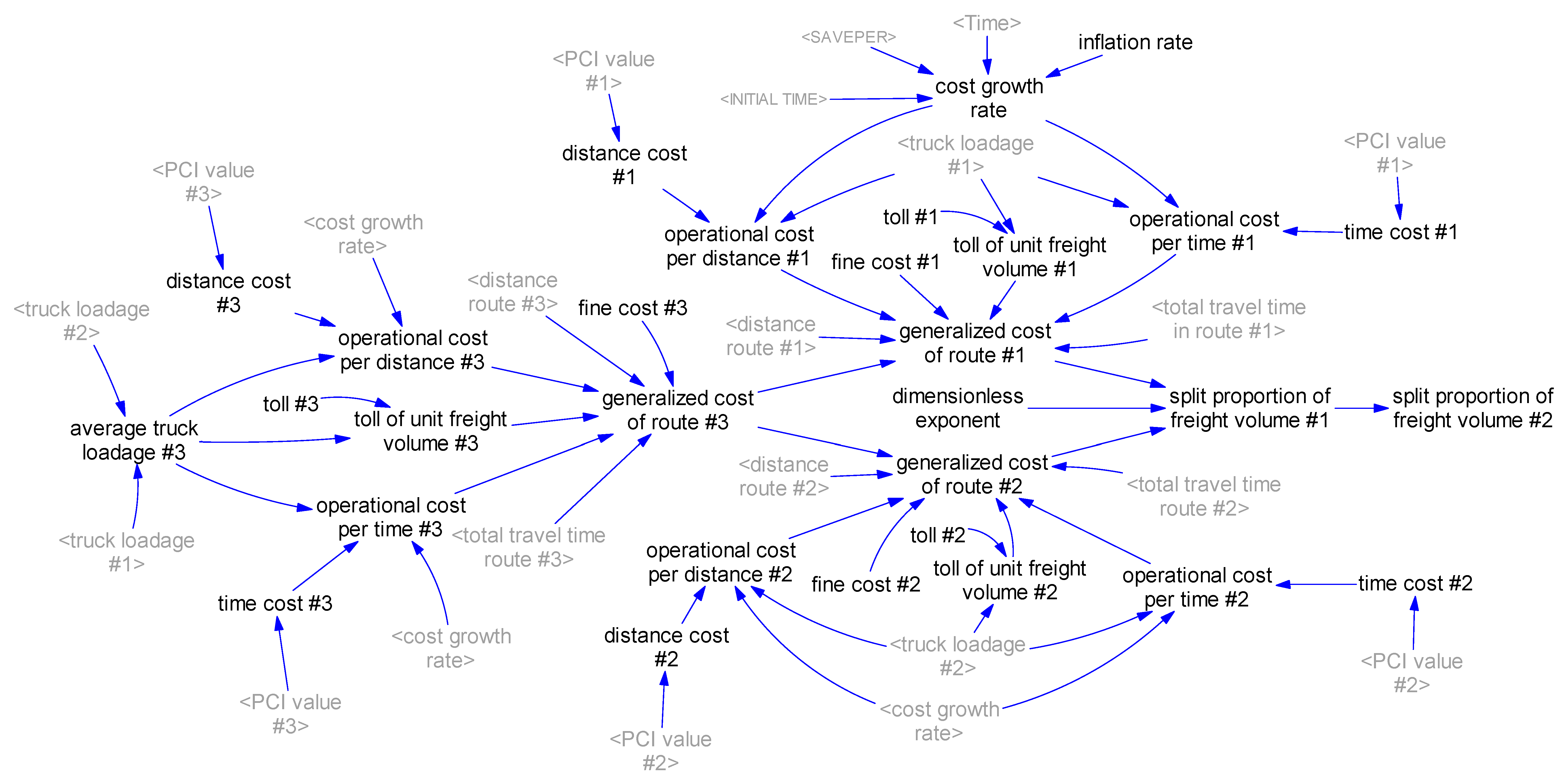
The module “Modal Split,” shown in Figure 4, uses travel time and distance, besides the transportation operational cost in function of the distance and time for each pavement condition, whose objective is to calculate the proportion of load volume to be transported in each route. In this module, the modal choice refers to the choice of the route to be used, determined by the multinomial logit function employed in the modal split model [42]. This way, the proportion of freight volume transported through Route #1 is given by Equation (2).

$$Split proportion of freight volume \#1=ex{p}^{\left(-c1\right)}/\left({\displaystyle \sum }_1^{n}ex{p}^{\left(-c_n\right)}\right)$$

(2)

where:

• c1: generalized cost of Route #1; and
• n: number of available routes.

Generalized cost depends on the type of vehicle and on the physical and operational conditions of the road and is made of parts that vary according to the distance traveled, travel time and other fixed costs, such as tolls and other fine costs [43]. Equation (3) is used to calculate generalized operational cost.

$$G{C}_{v,r,p}={\beta }_1·\left(T_{v,r,p} · C{T}_{v,r,p}\right)+{\beta }_2·\left(L_{r,p} · C{L}_{v,r,p}\right)+{\beta }_3·(C{T}_v)+{\beta }_4·(C{F}_v)$$

(3)

where:

• GCv,r,p: generalized cost generated by a vehicle v while traveling a link of category r,p (r = type of terrain and p = pavement condition);
• Tv,r,p: time traveling through the link of category r,p by the vehicle v;
• CTv,r,p: parameter of operational cost per time unit required for vehicle v to travel a link of category r,p;
• Lr,p: length of link of category r,p;
• CLv,r,p: parameter of operational cost per unit of distance required for vehicle v to travel a link of category r,p;
• CTv: toll cost of the link for a vehicle of class v, which may be zero, in the absence of a toll or the fare value, in case there is a toll station in the link;
• CFv: fine costs for driving overloaded vehicle of class v; and
• ${\beta }_1,{\beta }_2,{\beta }_3\mathrm{and}{\beta }_4$: perception weights.

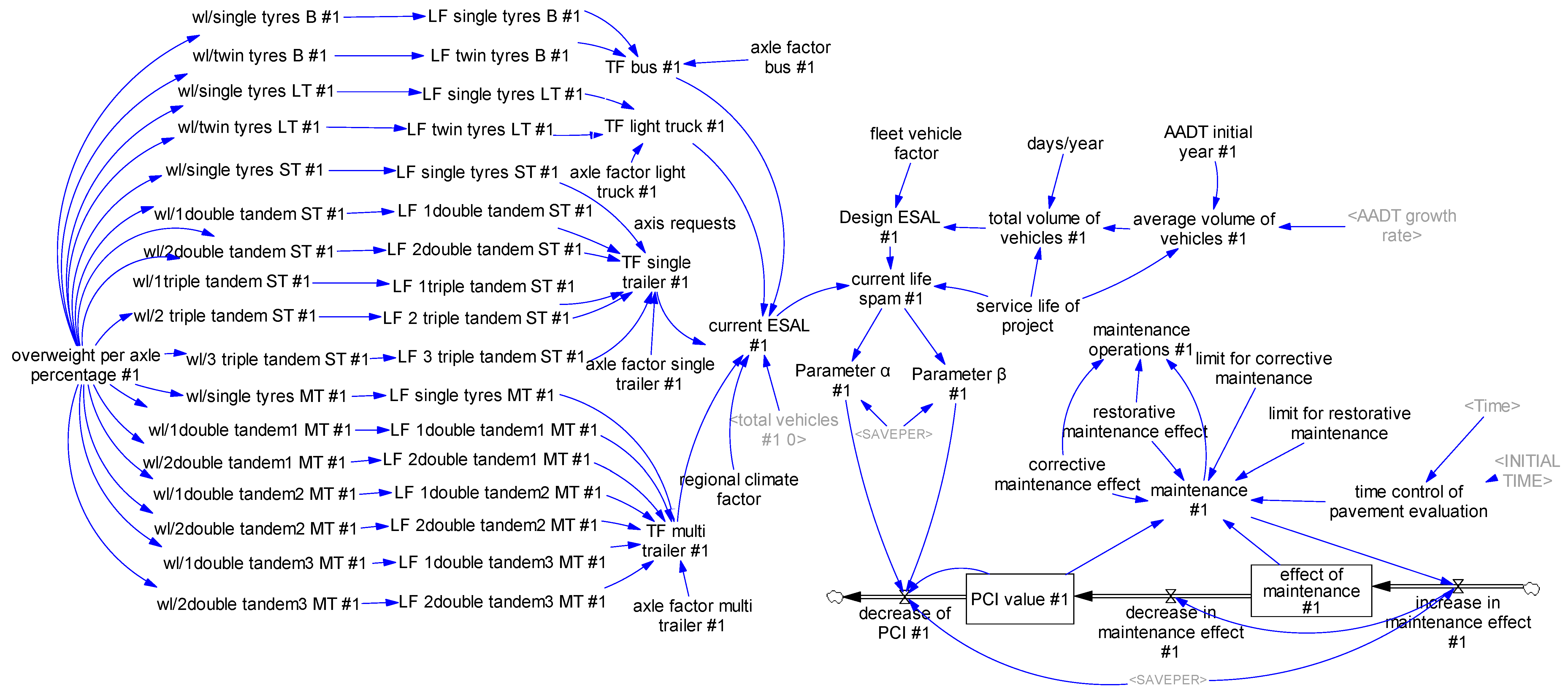
In the “Pavement Maintenance” module, presented in Figure 5, the Pavement Condition Index (PCI) determines if the maintenance operations may be of corrective or restorative types. The Design ESAL is the number of demands made by a standard axle, based on the Annual Average Daily Traffic (AADT), on its growth rate, on the project’s life span and considering the weight limits per axle, represented by the fleet truck factor (TF). Knowing the Design ESAL, the current life span of the pavement is calculated in function of traffic demand. The accelerated degradation and the reduced life span of the pavement are caused by excess weight per axle. For that reason, it was necessary to characterize the composition of heavy vehicle traffic of the analyzed routes.

To calculate the Load Factors (LF), the AASHTO method [12] was used, considering the weight per axle with the allowed tolerance and the excess weight percentage practiced. The reduced life span is related to the PCI through the parameters α and β, related to pavement performance [44]. The PCI measures the quality of the pavement and accumulates the difference between the effect of maintenance and the decrease in PCI caused by vehicle traffic.

The first maintenance condition is the current pavement quality level, that is, if the current PCI is higher than the limit that requires the conduction of corrective maintenance, there is no need for pavement intervention at that given moment of time. The second condition for the requesting of interventions is the absence of any ongoing maintenance operation. Finally, the request for maintenance interventions must respect the time interval in which no assessments of pavement conditions are carried out. Considering these three conditions, if the PCI is within the limits for restorative and corrective maintenance, corrective maintenance is made. If the PCI is under the limit for restorative maintenance, this type of maintenance is made.

The stock effect of maintenance accumulates the input of such effect, which occurs when the maintenance is requested but with a delay in the application of such effect on PCI due to the considerable time needed to carry out the works. The variable maintenance operations are defined by the values 1 and 0.5 for restorative and corrective maintenance operations, respectively and zero if there is no need for pavement intervention.

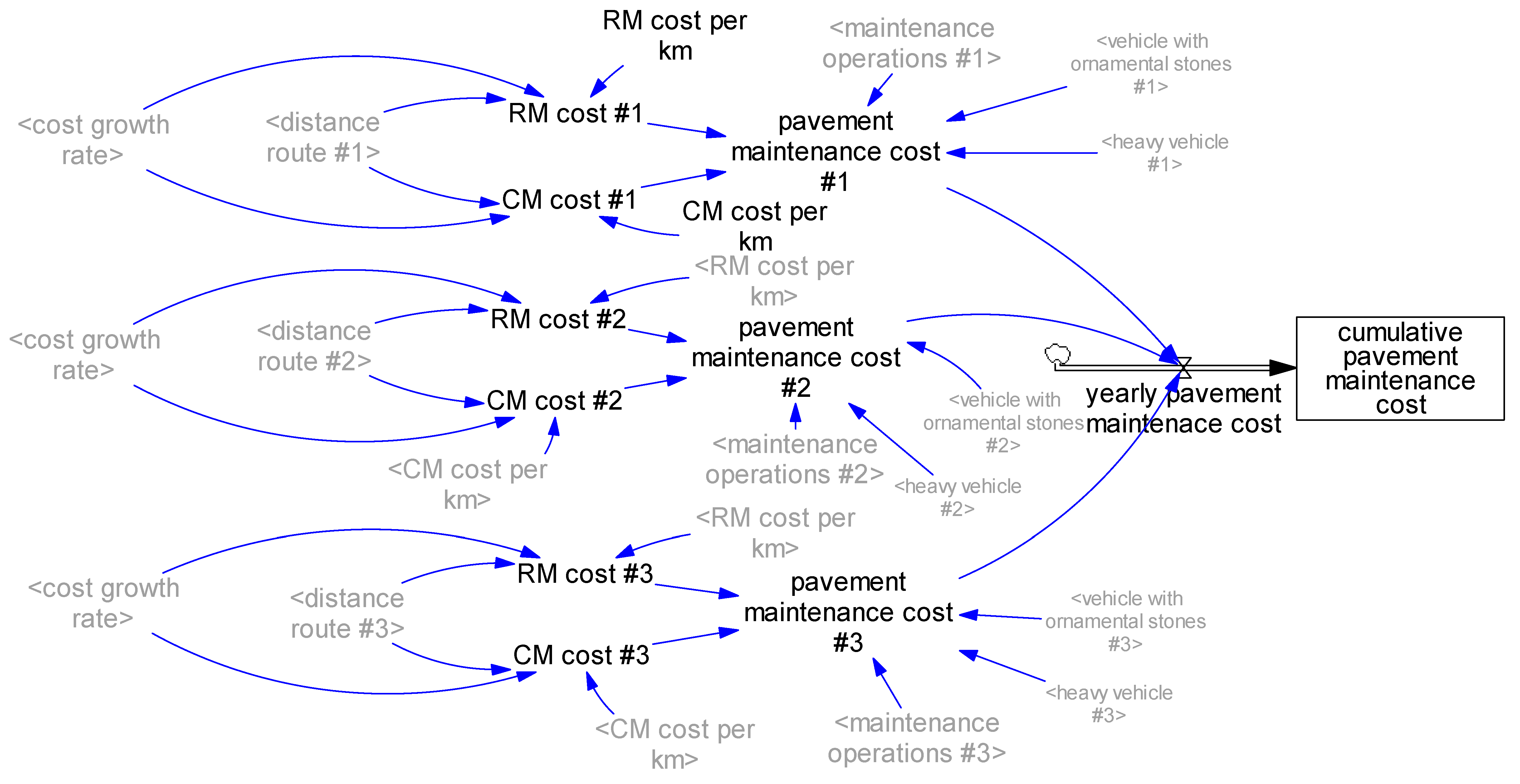
The fifth stock and flow module shows the “Social Cost of Freight Transportation,” which is subdivided into pavement maintenance costs and traffic accident costs. Figure 6 shows the stock and flow diagram for pavement maintenance costs.

The stock type variable “cumulative pavement maintenance cost” accumulates the yearly cost with pavement maintenance throughout the whole simulation period. The flow variable “yearly pavement maintenance cost” is the sum of all costs with maintenance in each of the analyzed routes. The costs with corrective maintenance (CM) and restorative maintenance (RM) are defined by the cost per kilometer, the distance of the route and the cost growth rate, as shown in Equations (4) and (5).

$$CM cost \#1=CM cost per km · distance route \#1 · cost growth rate$$

(4)

$$RM cost \#1=RM cost per km · distance route \#1 · cost growth rate$$

(5)

Finally, the pavement maintenance cost is calculated in function of the type of intervention to be carried out, defined on previous module and their related costs, as shown in Equation (6).

$$\begin{gathered} pavement maintenance cost=IF THEN ELSE(“maintenance operations”=0, 0, \\ IF THEN ELSE\left(“maintenance operations”=0.5,\left(“CM cost” \right),\left(“RM cost” \right)\right)) \end{gathered}$$

(6)

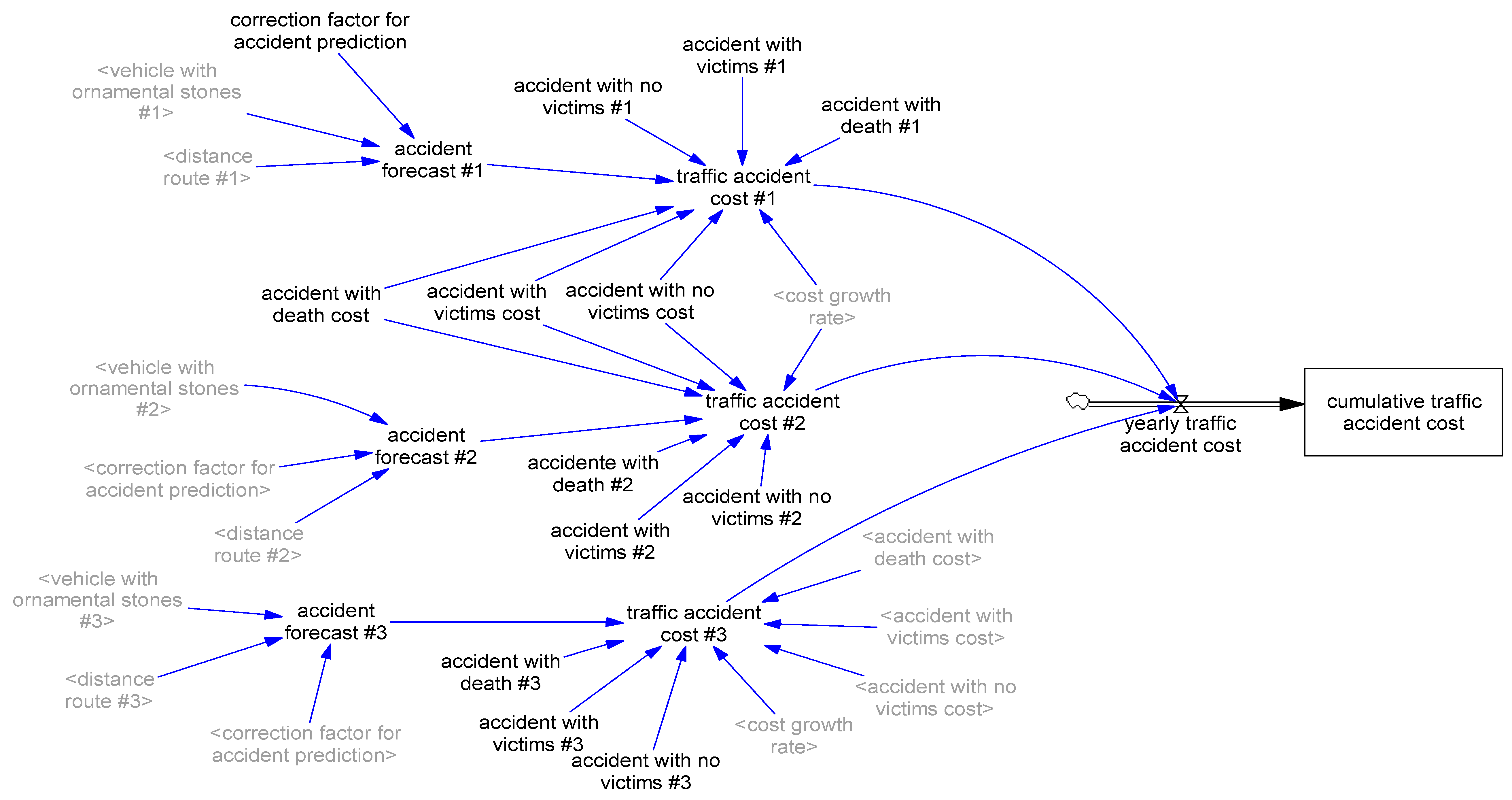
The second part of the “Social Cost of Freight Transportation” module addresses the costs with traffic accidents, as shown in the stock and flow diagram presented in Figure 7. The variable “cumulative traffic accident cost” accumulates the yearly costs with traffic accidents throughout the simulation period. The flow variable “yearly traffic accident cost” is the sum of the costs with accidents per year in the analyzed routes, which is given by Equation (7).

$$\begin{gathered} traffic accident cost \\ =accident forecast · ({\displaystyle \sum }_{i=1}^3\left(\% accident level i · cost accident level i\right)· cost growth rate \end{gathered}$$

(7)

The prediction of accidents is defined in function of the AADT, which regards to the overloaded vehicles and the traveled distance, according to the accident prediction model proposed by the Highway Safety Manual User Guide—HSM [45], as shown in Equation (8).

$$\begin{gathered} accident forecast \\ =overloaded vehicle · distance route·{10}^{\left(-6\right)}·ex{p}^{\left(-0.312\right)}·correction factor accident pred \end{gathered}$$

(8)

The correction factor for accident prediction is needed and it is indicated by the HSM in case the analyzed routes are not under the ideal conditions indicated by the manual. Therefore, the accidents are dependent of both limit of the vehicles and conditions of the highways.

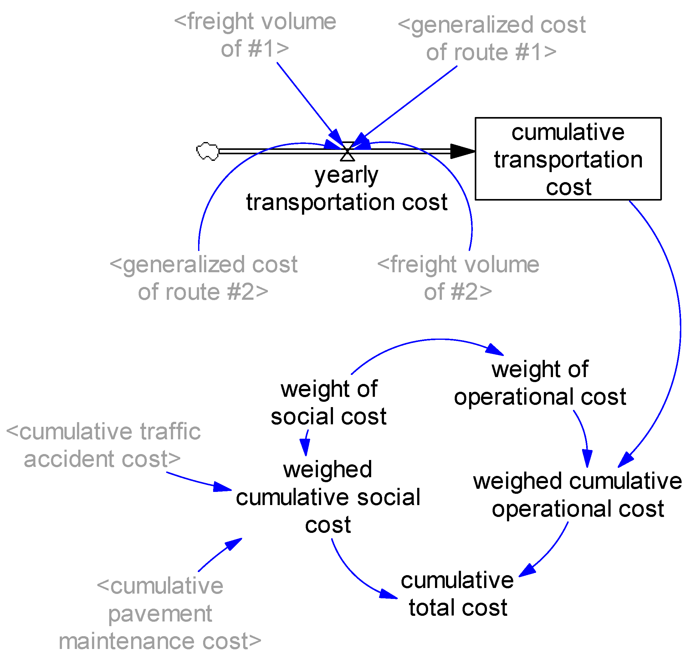
Finally, the sixth module, “Policy Assessment,” receives the road maintenance costs, the accident costs and the generalized cost of each route to calculate the cumulative total cost. Then it is able to simulate scenarios with importance weights attributed to the costs (operational and social) in function of different loading policies for freight vehicles in overload percentage. Figure 8 shows the stock and flow diagram for this module.

The variable “cumulative transportation cost” accumulates the yearly transportation costs of the available routes. The weighed cumulative operational cost is given by the stock of cumulative transportation cost and the weight (relative importance) of such cost. Likewise, the weighed cumulative social cost is given by the sum of pavement maintenance costs and accident costs, multiplied by the weight of social costs. Finally, cumulative total cost is the sum of the weighed cumulative operational and social costs of all routes involved.

This way, it is possible to assess the impact caused by varying overweight percentages in freight vehicle loading on total system cost, as well as by varying the importance attributed to each type of cost by decision makers.

3.2. Mathematical Formulation

The next step of SD methodology is the development of the mathematical model, which consists in transforming the stock and flow diagram into a system of differential equations, solved via simulation by numerical integration. The model was structured in Vensim PLE^® software—a free software from the company Ventana Systems [46] intended for personal and educational use. The mathematical equations and the model can be obtained at supplementary materials.

3.3. Model Testing

The proposed simulation model fits in the quantitative modeling category, since it involves inductive formulation and model simulation focused on the comprehension of stock and flow structures and applied to the representation of quantifiable systems [32]. The tests considered most appropriate to this modeling category are: physical conservation, dimensional consistency, integration error, extreme conditions tests, boundary adequacy tests, parameter assessment, basic behavior reproduction and endogenous behavior reproduction tests.

During the formulation of the model, simulations were carried out to verify the physical conservation of the model’s structure. For example, Figure 9 shows the stock of the PCI, in which it is possible to see that the index decreases until receiving the effect of restorative maintenance in 2022 (100 points) and corrective maintenance in 2028 (80 points). The stock does not become negative, satisfying the expected behavior.

Dimensional consistency is the specification of the units of measurement of the variables throughout the formulation of the model and the verification of their physical meaning using mathematical equations [22]. To carry out this test, the command “Check Units” of the Vensim software was used. All inconsistencies were solved during the formulation of the model until the dimensional adjustment of all variables involved in the proposed model.

Besides, some variables were replaced with internal variables such as “Time” (current simulation time), “Initial Time” (initial simulation time) and “Saveper” (time interval in which simulation results are saved), the units of which are defined the same as for the simulation model horizon, given in years. This way, the communication and comprehension of the model was facilitated.

For the proposed model, Euler’s integration method was used due to the low amount of computational time required by it and its high numeric stability [47]. In the integration error test, the model should be executed with an initial estimate for d_t and this value should be progressively reduced by half until there are no significant changes to the model’s behavior. The time step chosen for the model was of ¼ of a year. This choice was made based on simulations with different values of time step for the variable “Total traffic #1.” A difference of 1% was considered acceptable for the total traffic during one year in the considered route. This way, the chosen time step was of 0.25 year, since, when the time step is changed from 0.25 to 0.125, the change in behavior is lower than 1%.

The extreme conditions test checks whether the model has an appropriate behavior when the parameters are submitted to extreme values, such as zero or infinite and may be carried out in two ways: via the direct inspection of the model’s equations or via simulation [22]. The variables submitted to extreme values for this test and the behavior expected for the verification are shown in

Table 1. Variables for the extreme conditions test.

Module	Variable	Value	Behavior Expected
Load volume forecast	Initial stock of Total freight volume	0	Absence of vehicles for stone transportation and their effects over costs
	Initial stock of freight volume #1 and freight volume #2	0
Speed Flow	Maximum capacity	10	Increase in average travel time
Modal split	Toll #1	1.000	Proportion of freight volume in Route #1 will be null
Pavement maintenance	Overweight percentage per axle	10.000	Current life span will be null
	Project life span	0	PCI value will be null

. After conducting the tests via simulation, all the behaviors expected under the established extreme conditions were respected, which confirms the reliability of the proposed model’s structure.

The boundary adequacy test checks whether the limits of the model’s boundaries are adequate for the simulation purpose. For that, it is possible to directly inspect the model’s equations, but the diagrams of causal relationships and stock and flow facilitate the identification of exogenous constants that should be considered variables of the model. If an additional structure has a significant impact over the behavior or political implications, it must be included as an integral part of the model [22].

Road capacity was initially considered an input parameter external to the model. However, since this parameter influences route travel times, it was chosen to include the calculation of road capacity in the model, using the HCM as a reference [40]. It was also decided that the calculation of the Design ESAL should be included, since it impacts the reduction in pavement life span and the decision about road maintenance requests. Therefore, the limits of the model were expanded and adjusted as needed throughout its construction and formulation considering the desired objective.

The tests of parameter assessment, basic behavior reproduction and endogenous behavior reproduction were not carried out due to the absence of historical data about the AADT for the analyzed road network of the case study. However, the tests conducted make it possible to conclude that the model is capable of obtaining results and simulating scenarios.

4. Case Study

The case study approaches the transport of ornamental stones in the state of Espírito Santo (Brazil). This model considered the characteristics related to the Brazilian reality, in which the roads are used by various vehicle categories and all of them significantly impact travel time, pavement conditions and operational costs of the routes used.

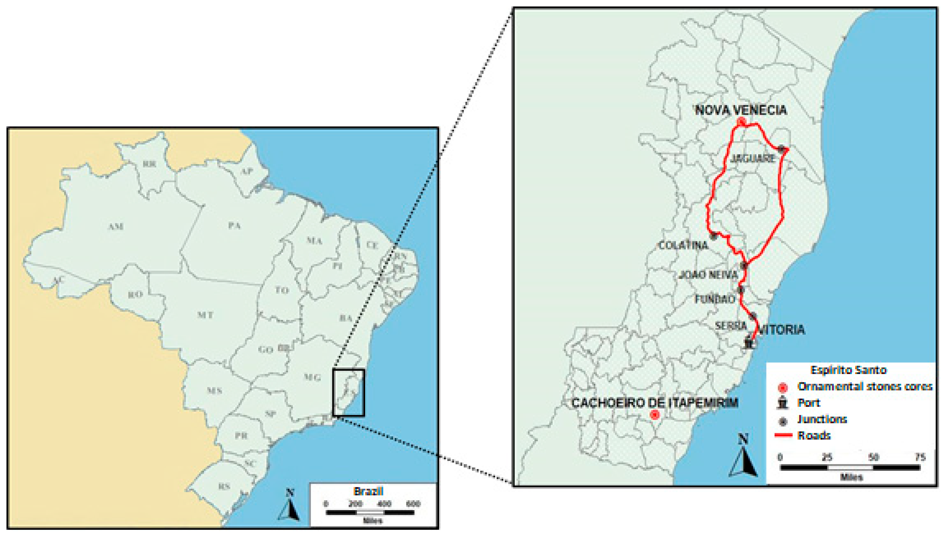
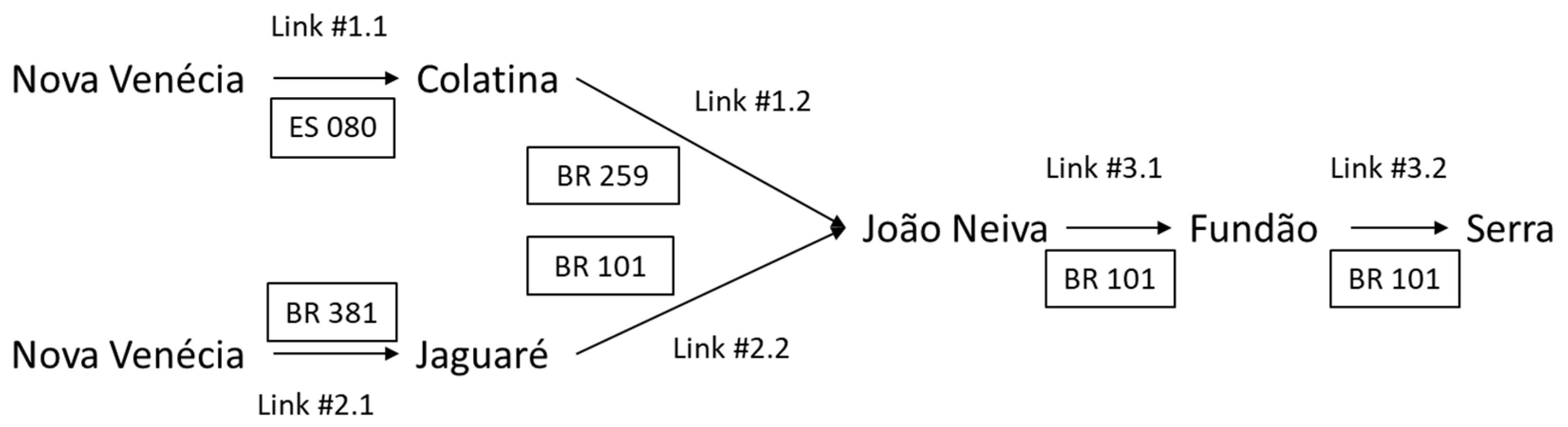
The state of Espírito Santo, which is in the Southeast region, shown in Figure 10, stands out in the national scenario of ornamental stones because it has the largest reserve of marble in the country and a large reserve of granite. The two main regions in this sector are: the southern state region and the northwestern region, whose reference is the city of Nova Venécia, with a large production of granite and a high concentration of businesses in both extraction and processing [48].

Considering that around 70% of all granite exported by Espírito Santo comes from the northwestern region of the state [49], the object of this study was the transportation of ornamental stones from Nova Venécia to the port of Vitória. The access to the productive center of the city of Nova Venécia may occur via two main road routes, through which the production of ornamental stones is transported to the port of Vitória, according to Figure 11.

However, the links that comprise each road have specific characteristics that need to be considered, such as Annual Average Daily Traffic (AADT) and road capacity, as indicated by Reference [12], since the different vehicle categories and the volume of traffic that use the roads significantly impact pavement conditions, trip time and the operational cost of using these routes.

To characterize the AADT, in 2014, DNIT resumed the National Plan of Traffic Count (PNCT—Plano Nacional de Contagem de Tráfego in Portuguese), which identifies traffic behavior on federal paved roads. Besides defining a systematic traffic count plan using permanent count devices in federal roads, in 2016 and 2017 DNIT conducted Traffic Count and Classification surveys and Origin and Destination surveys to collect information on vehicle flows on federal roads [50]. This way, the ornamental stones transportation routes analyzed in this study were divided in links according to the homogeneity of traffic volume, as illustrated by each junction in Figure 11.

Route #1 (link #1.1 and link #1.2, see Figure 11) does not have weight inspection via fixed scales, which facilitates the practice of overloading. However, freight vehicles that use Route #1 may eventually be submitted to inspection with mobile scales operated by DNIT. Moreover, Route #1 does not have tolls either, which influences the users’ choice for this route.

Route #2 (link #2.1 and link #2.2) has a fixed scale on the flow direction analyzed in this study, that is, from north to south. However, inspections at the fixed scales are subject to the scheduling and availability of inspectors belonging to the responsible agency in the state, that is, they do not operate continuously. Besides, Routes #2 and #3 (link #3.1 and link #3.2) have tolls.

Therefore, it is initially assumed that legal weight limits per vehicle are respected in Route #2 but there is also the possibility of overweight being practiced in this route considering the inconsistency of inspection in it. Therefore, considering that overweight was identified as a recurring problem for the road transportation of ornamental stones in the state of Espírito Santo, this article presents a SD model to analyze the relationship between overweight vehicle and the costs associated, such as operational transportation costs and social costs with road accidents and pavement maintenance.

Thus, we present the values of the specific constants in each module for the application of the proposed case study.

4.1. Parameters for the Load Volume Forecast Module

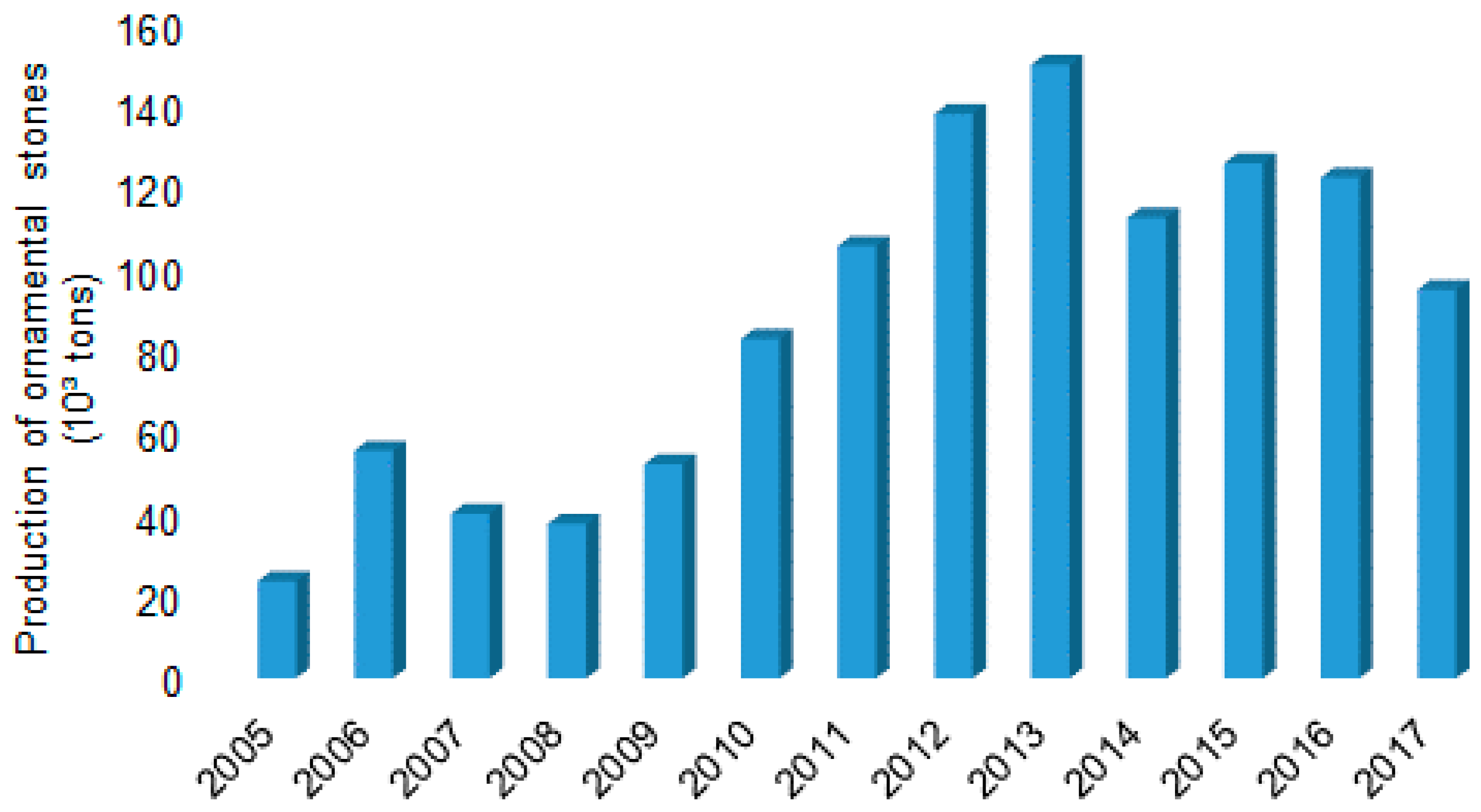
For the first module, it is necessary to obtain the freight volume growth rate. For that, data on the exports of ornamental stones in the municipality of Nova Venécia were used [51] and it is known that an average of 34% of the Brazilian production of stones was destined to the foreign market between 2005 and 2008 [52]. Thus, it is possible to estimate the production of stones in the municipality of Nova Venécia based on the export values [53], as shown in Figure 12.

There is an observable growth in the production of stones in the period between 2008 and 2013 and an oscillation in the remaining periods, with an overall growth average of 8% a year. When the year of 2017 is disregarded, since the base year for the beginning of the simulation is 2016, the growth percentage is of 11% a year, value used in the simulation.

4.2. Parameters for the Speed Flow Module

For the “Speed Flow” module, it is necessary to find the AADT of each link of the analyzed routes, retrieved from the PNCT project [50]. For each analyzed link, the average volume of the sub-links of the National Traffic System were considered. Thus, the volume of light and heavy vehicles, identified in the model’s base year of simulation (2016), is summarized in

Table 2. Estimate of the average AADT (vehicles) of each link in 2016.

Routes	Links	Distance (Km)	Light AADT	Heavy AADT	Total AADT
#1	#1.1	123	998	365	1.363
	#1.2	45	1.784	609	2.394
#2	#2.1	65	947	388	1.335
	#2.2	110	3.385	1.293	4.678
#3	#3.1	38	4.956	2.289	7.245
	#3.2	26	6.515	2.030	8.546

Source: Authors based on Reference [50].

.

According to the Traffic Studies Manual [12], the traffic has relatively low variation in annual growth rates. According to the manual, it has become common to adopt an annual growth rate of 3%, adopted in the simulation model.

For the transportation of ornamental stones, there are several configurations of vehicle axles, whose Total Gross Weight (TGW) limit varies from 23.1 to 77.7 tons. However, according to Resolution nº 354/2010 [54], the vehicle adopted as the standard vehicle for the transportation of stones was a special multitrailer of seven axles (three dual tire tandem axles and a one-tire single axle) with a Combined Total Gross Weight of 57 tons.

Given the legal limit of vehicle loading and the volume of ornamental stones to be transported, it is possible to find the traffic of stone transportation vehicles, which will be added to the traffic of other vehicle categories. This aspect of the model is also different from the models found in literature review, in which the authors consider only the traffic of specific vehicles, which is not consistent with the Brazilian reality.

For information regarding the overweight practiced in the transportation of ornamental stones on the analyzed routes, this study used data regarding weighings carried out by mobile scales operated by DNIT on roads in the state of Espírito Santo between 2015 and 2017. Data showed that the percentage of overweight in TGW varied from 0.05% to 57.20%, already considering the 5% tolerance defined in the legislation. Overweight per axle, in turn, varied from 0.25% to 70.70%, already considering the 10% weight tolerance per axle, as defined in current legislation. The operational speed of 80 km per hour (Km/h) was considered for the free flow time on the links.

4.3. Parameters for the Modal Split Module

The operational cost associated with each of the analyzed routes was found based on the HDM-4 methodology [43]. The operational costs vary according to the type of vehicle, the type of guideway, pavement condition and type of terrain. These differences lead to different travel times for the same distances, which may affect transportation route choice via the road mode. Moreover, the operational costs were calculated for the following combination of standard links:

• Roads (5 types): Multilane highways, wide lane (two-lane highways with paved at-grade shoulder), federal two-lane highway, state two-lane highway and unpaved highway;
• Pavement (4 types): Good, fair, mediocre and poor, defined according to the IRI (International Roughness Index [55]; and
• Terrain (5 types): level, slightly rolling, rolling, very rolling and mountainous, defined through the vertical and horizontal geometry indices.

The maintenance items considered were the following: fuel, lubricants, tires, maintenance (parts), workforce, depreciation and crew costs (freight vehicles). The first four of these items are related to the distance traveled and the remaining ones to the time needed to travel this distance. Thus, it is possible to arrive at a set of unit costs that vary according to the distance and a set of unit costs that vary with time [43], as previous shown in Equation (3).

There is information about Routes #1, #2 and #3 concerning the type of lane and terrain on the georeferenced database for project PNCT [50]. The vehicle class chosen was the multitrailer with 7 axles and the costs per distance and per time (cost used in first and second terms of Equation (3)) were determined in function of the variation in pavement condition, as presented in

Table 3. Operational costs per distance and time in relation to type of lane, pavement condition and type of terrain for a multitrailer with 7 axles.

Routes	Type of Road_Condition_Terrain	PCI	Cost per Distance (R$/Km)	Cost per Time (R$/H)
#1	Two-Lane_Good_Rolling	100	1.58	83.91
	Two-Lane_Fair_Rolling	75	1.73	83.06
	Two-Lane_Mediocre_Rolling	50	1.91	79.61
	Two-Lane_Poor_Rolling	25	2.10	72.93
#2	Two-Lane_Good_Rolling	100	1.53	72.19
	Two-Lane_Fair_Rolling	75	1.67	71.20
	Two-Lane_Mediocre_Rolling	50	1.84	67.94
	Two-Lane_Poor_Rolling	25	2.03	63.05
#3	Two-Lane_Good_Very Rolling	100	1.63	64.04
	Two-Lane_Fair_Very Rolling	75	1.77	63.86
	Two-Lane_Mediocre_Very Rolling	50	1.94	63.28
	Two-Lane_Poor_Very Rolling	25	2.12	61.18

Source: Reference [43].

.

Routes #1 and #2 are predominantly made of two-lane and rolling terrain and Route #3 is predominantly made of two-lane and very rolling terrain. For each type of lane and terrain, pavement conditions may be good, fair, mediocre and poor and they were related to the PCI with the values 100, 75, 50 and 25, respectively.

Table 3 shows that, as pavement conditions worsen, with a decrease in the PCI, the cost per distance increases due to fuel, lubricant and tire consumption and to maintenance parts. Cost per time, which is related to workforce, depreciation and crew costs, decreases as the PCI also decreases. This may be explained by the fact that, when pavement conditions worsen, vehicle speed decreases and, consequently, travel time increases. Therefore, associating fixed costs with a longer travel time, costs per time are lower when the PCI decreases.

The third parameter of Equation (3) is the toll cost. The values shown in

Table 4. Toll fares in the analyzed routes for a truck of 7 axles.

	Municipality	Location	Value (R$)
Route #2	Aracruz	Highway BR 101, Km 171.7	30.00
Route #3	Serra	Highway BR 101, Km 242	28.80

Source: Reference [56].

refer to the toll in each route and were retrieved from the website of the concessionaire [56].

The last parameter of Equation (3) is the fine cost, related to the fines for driving overloaded vehicle, for example. However, this cost was disregarded in this case study because we do not have access to this kind of data and also because the scales are not operating continuously on the roads under study. Besides, the perception weights (${\beta }_1,{\beta }_2,{\beta }_3\mathrm{and}{\beta }_4$) are parameters difficult to be defined. In our case study, we used one for all of them.

The Inflation rate determines the growth rate of operational costs in transportation, as well as the other costs in other modules of the model, such as traffic accident and pavement maintenance costs. The Extended Consumer Price Index—IPCA, produced by the Brazilian Institute of Geography and Statistics, is the country’s official inflation index. In 2016, the IPCA had a growth of 6.29% [57], thus, this percentage was used for the initial inflation rate.

4.4. Parameters for the Pavement Maintenance Module

For the module “Pavement Maintenance,” it is necessary to determine the AADT of the base year used in each of the three routes. Considering that each route is subdivided into two links, the calculation of the Design ESAL used the highest AADT of each route, which is shown in Table 2. The AADT Growth rate was obtained from the “Speed Flow” module and the Fleet vehicle factor was obtained from the model itself as the sum of the Vehicle Factors of each category in the scenario in which the percentage of overweight per axle is null.

For the calculation of the base year’s Design ESAL, it was necessary to differentiate the percentage of each category of heavy vehicles in the vehicle fleet based on the samples of Traffic Count and Classification surveys [50] carried out at the links under analyze. The following four categories representing heavy vehicles were chosen to calculate the Design ESAL: buses, light trucks, semitrailer and multitrailer.

The respective representations and the total number of axles for each selected vehicle category are shown in

Table 5. Configuration of the representative categories used to calculate Design Traffic.

Representation	Category	Configuration of Axles	Axles
	Bus (B)	Single tyres on front axle Twin tyres on rear axle	2
	Light truck (LT)	Single tyres on front axle Twin tyres on rear axle	2
	Semitrailer (ST)	Single tyres on front axle of tractor Twin tyres on both rear axles of tractor (double tandem) Twin tyres on three rear axles of trailer (triple tandem)	6
	Multitrailer (MT)	Single tyres on front axle of tractor Twin tyres on both rear axles of tractor (double tandem) Twin tyres on axles of trailer (double tandem)	7

Source: Reference [58].

. The weights legally allowed for each type of axle, considering the tolerance, are shown in

Table 6. Weight limits, considering the tolerance of 10% per axle.

	Weight Allowed per Axle Group (t)	Total (+ Tolerance 10%)	Weight per Axle
Single tyres	6.00	6.60	6.60
Twin tyres	10.00	11.00	11.00
Double tandem	17.00	18.70	9.35
Triple tandem	25.50	28.05	9.35

Source: Authors based on References [59,60].

.

To decide about the type of maintenance that will be performed on the pavement, the limits for corrective and restorative maintenances are defined in function of the IRI, recommending an IRI value higher or equal to 3.5 as a “trigger” for pavement maintenance interventions [61]. It is recommended to correlate these indexes with the PCI by means of a subjective assessment, as shown in

Table 7. Relationship between the pavement performance index and the irregularity indexes.

Assessment	Irregularity	Condition	Interventions	Effects
	IRI (m/Km)	PCI (points)	Maintenance	PCI (points)
Very Good	1–1.9	100	-	-
Good	1.9–2.7	80	-	-
Fair	2.7–3.5	60	-	-
Mediocre	3.5–4.6	40	Corrective	80
Poor	>4.6	20	Restorative	100

Source: Adapted by Reference [61].

.

Thus, the limits for corrective and restorative maintenance interventions in relation to the PCI are of 40 and 20 points, respectively. In case the corrective maintenance is carried out, the PCI increases to 80 points. If restorative maintenance is required, the PCI level increases to 100 points.

Finally, we do not have data costs of the pavement condition surveys but they are not carried out every year. Thus, it was chosen to simulate the time interval between two PCI surveys, varying from 2 to 5 years and the duration of maintenance works, also varying from 2 to 5 years.

4.5. Parameters for the Social Cost of Freight Transportation Module

The “Social Cost of Freight Transportation” module is divided into pavement maintenance cost and traffic accident costs. To determine pavement maintenance costs, it is necessary to determine corrective maintenance cost per kilometer (CM/Km) and restorative maintenance cost per kilometer (RM/Km). For that, DNIT published the average management costs for the road mode, as shown in

Table 8. Pavement maintenance costs.

Maintenance	Lower Limit (R$/Km)	Upper Limit (R$/Km)	Average (R$/Km)
Corrective	566,577.08	1,761,708.99	1,164,000.00
Restorative	1,783,916.27	2,883,935.73	2,334,000.00

Source: Reference [62].

.

For road accident costs, the Institute of Applied Economic Research—IPEA [63] presented an overall characterization of accidents in Brazilian federal roads, analyzing the evolution of their costs based on data from the Federal Road Police—PRF for the base years 2007, 2010 and 2014. The CNT [64] updated the study based on the number of accidents registered in 2015 and on the inflation for the period, as shown in

Table 9. Total cost and average cost per accident severity.

Severity	Average Cost (R$/occurrence)
Accident with death (AD)	715,772.55
Accident with victims (AV)	99,805.21
Accident with no victims (ANV)	25,523.79

Source: Reference [64].

.

Costs with traffic accidents are associated with people, vehicle or property damage and institutional costs. Costs associated with victims regarding hospital costs and loss of production, that is, how much income traffic victims stop earning both during the period they are away from economic activities and, in case of death, regarding their life expectancy. Costs associated with vehicles depend on vehicle category (cars, motorcycles, bicycles, vans, trucks, buses and others) but are represented by removal, property damage and freight loss. Finally, institutional costs refer to costs with care and property damage [63].

To define the percentage of each type of accident according to severity, data from PRF [65] were used which consider the accidents that occurred in the links of federal roads belonging to the routes analyzed in the year 2016, as shown in

Table 10. Number and percentage of accidents according to severity.

Highway	Severity	Number of Accidents	Percentage (%)	Accidents average/Km Federal Link	Estimate State Link	Total
BR 259 0 (Link #1.2)	AD	13	11	0.3	36	49
	AV	89	75	2.0	243	332
	ANV	17	14	0.4	46	63
	TOTAL	119	100	2.6	325 1	444
BR 101 0 (Link #2.2)	AD	15	3	0.1	9	24
	AV	367	82	3.3	217	584
	ANV	65	15	0.6	38	103
	TOTAL	447	100	4.1	264 2	711
BR 101 0 (Route #3)	AD	34	4	0.5	-	34
	AV	641	76	10.0	-	641
	ANV	173	20	2.7	-	173
	TOTAL	848	100	13.3	-	848

Note: ¹ Estimate of accidents for link #1.1 and ² Estimate for link #2.1. (Source: Reference [65].)

.

The estimate of the number of accidents in the links of state highways of Routes #1 (Link #1.1) and #2 (Link #2.1) was made using the average of accidents per kilometers in federal highways, multiplied by the length of the state highway link. Next the number of accidents of federal road links was added to the estimated number of accidents in state road links.

The accident prediction model proposed by the HSM [45] suggests a correction factor when the road conditions are not ideal. To find out the correction factor, the model was simulated considering a scenario in which road and traffic conditions are ideal, that is, accident prediction was based only on AADT and route length. Next, the real number of accidents was divided by the number of accidents under ideal conditions to find out that the average correction factor for the accident prediction model of each route was 8.5, that is, the real number of accidents is in average 8.5 higher than the number predicted by the model under ideal conditions.

5. Results and Discussions

The simulation period was of 15 years, corresponding to the average pavement duration time and is compatible with the economic analysis needs regarding the interval between 2016 and 2030. After 15 years, in normal conditions, a surface renovation would be expected [66].

Table 11. Description of scenarios.

Scenario	Simulated Variables	Impact
1. Reference	Time control in pavement assessment (2, 3, 4 and 5 years)	Maintenance; Cumulative cost of pavement maintenance
	Output flow delay due to maintenance (2, 3, 4 and 5 years)
2. Strict, Moderate and Tolerant Policies	Overweight percentage from 0 to 100% (Increment of 10%)	Cumulative cost of transportation, pavement maintenance and traffic accidents; Total cumulative cost
3. Assessment of the Best Policy	Overweight percentage and Weight of social cost	Total cumulative cost
4. Overweight in all routes	Overweight percentage	Cumulative cost of pavement maintenance; cumulative cost of transportation; cumulative cost of accidents

summarizes the proposed scenarios, the simulated variables and the impact analyzed in each scenario, which are detailed below.

In Scenario 1 (Reference Scenario), different values were simulated for time control in pavement assessment with intervals of 2 to 5 years between them and the delay in the effect of maintenance, that is, the duration in years of maintenance works, also with intervals of 2 and 5 years. The analyzed effects refer to the number of maintenance requests and over cumulative pavement maintenance costs.

Scenario 2 was also simulated and compared to the Reference Scenario. Following the notation by References [37,38], three loading policies were adopted considering a variation of zero to 100% of overweight: Strict Policy (no overweight admitted); Moderate Policy (admits up to 50% of overweight); and Tolerant Policy (admits between 50% and 100% of overweight). The scenario with 100% overweight was hypothetical for simulation purposes. However, we note that there were already registrations of up to 70% in groups of axles and up to 57% in TGW. This implies in reducing road safety and other studies are recommended for a deeper analysis of these conditions.

Scenario 3 simulated variations of overweight percentage in vehicles and variations of the importance attributed to social costs simultaneously. With this, it was possible to identify the best vehicle loading policy (overload percentage) under different levels of importance attributed to social costs in relation to operational costs based on the minimization of the system’s total costs.

Finally, Scenario 4 addressed the practice of overweighting in all analyzed routes, regardless of the presence or operation of scales. This scenario was simulated to assess the impact over all costs considered in the model. The results of the proposed scenarios are presented as follows.

5.1. Reference Scenario

As presented before, the parameters simulated in the Reference Scenario are time controls in pavement assessment, that is, the interval in years between the gathering of pavement conditions to assess the need for maintenance and the delay in the output flow of the effect of maintenance or the duration of maintenance works. The variables impacted are Maintenance and Cumulative cost of pavement maintenance.

The delay in the output of the effect of maintenance regards the time spent in carrying out the maintenance works to increase the PCI. The reference used to define this maintenance time was the Program of Restoration and Maintenance Contracts—CREMA, which is subdivided into CREMA 1st step, with a duration of two years and CREMA 2nd step, with a duration of five years [67].

It was assumed that the assessment of pavement conditions is not carried out when a maintenance operation is in progress. This way, if the maintenance takes two years to be completed (delay), the assessment may be carried out in intervals of 2, 3, 4 and 5 years. On the other hand, if the maintenance has a delay of 3 years to be concluded, the assessment will not be carried out every 2 years, but it may be carried out in intervals of 3, 4 and 5 years.

Table 12. Maintenance and Total cost per route for each combination of time intervals of pavement maintenance and assessment.

Delay (Years)	Assessment Pavement (Years)	Maint. * Route #1	Total Cost Maintenance #1 (R$)	Maint. * Route #2	Total Cost Maintenance #2 (R$)	Maint. * Route #3	Total Cost Maintenance #3 (R$)
2	2	4 R	1,658,018,037	2 R and 1 C	2,427,611	4 R	182,418,339
	3	4 R	1,010,624,854	2 R	1,272,970	4 R	84,030,351
	4	3 R	878,864,580	1 R and 2 C	2,480,086	3 R	74,492,566
	5	2 R	388,020,604	2 R	1,575,210	2 R	28,275,918
3	3	2 R	251,825,934	1 R and 1 C	788,948	2 R	17,472,238
	4	3 R	876,486,084	2 R	1,703,138	3 R	74,492,573
	5	2 R	387,335,132	1 R and 1 C	1,522,382	2 R	28,275,918
4	4	2 R	724,094,260	2 R	1,703,138	2 R	64,026,375
	5	2 R	385,919,132	1 R	480,876	2 R	28,275,918
5	5	1 R	43,413,788	1 R	480,876	1 R	2,747,492

Note: * In this column, the letter “R” represents “Restorative” maintenance and the letter “C,” “Corrective” maintenance.

shows the amount and type of maintenance to be carried out and the total maintenance costs in each route after the simulation experiments that comprehended, as already mentioned, the period between 2016 and 2030.

Costs vary according to three characteristics: maintenance type; route length; and percentage of stone transportation vehicles in the analyzed route. For example, for a delay of 2 years in the effect of maintenance and an interval also of 2 years between pavement assessments, the following are required: 4 restorative maintenances in Route #1; 2 restorative maintenances and 1 corrective maintenance in Route #2; and 4 restorative maintenances in Route #3. Although Routes #1 and #3 receive the same amount of restorative maintenances, the cost is different due to the difference in route length and the percentage of stone transportation vehicles in relation to the total of heavy vehicles.

Furthermore, a route may also present different costs with the same amount of a same type of maintenance, as occurred with Route #1 under a delay of 2 years and intervals of 2 and 3 years between pavement assessments. In both cases, Route #1 required 4 restorative maintenances and, even so, the total maintenance cost in the period was different due to the different percentages of stone transportation vehicles that contribute to pavement degradation and its maintenance cost.

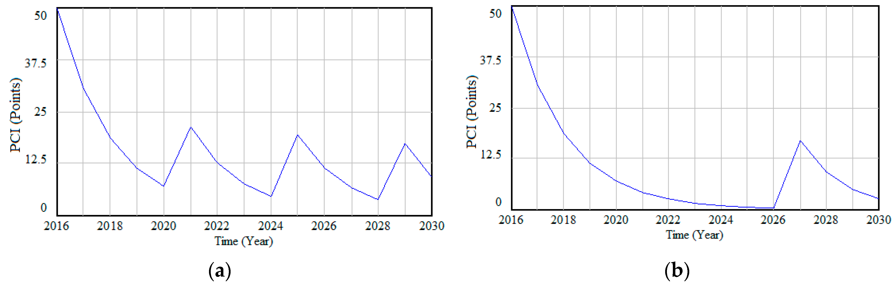
By analyzing the same intervals of pavement assessment, as maintenance delay increases, the number of maintenance requirements and, consequently, its cost decreases. The minimum pavement maintenance cost in all routes happens with the biggest interval of time between pavement assessments and the delay of the effect of maintenance. However, managers should decide about the trade-off between maintenance cost reduction and pavement performance index, which measures trafficability conditions in the road network. The bigger the time interval between pavement assessments, the lower the maintenance costs but also the worse the pavement conditions, as shown in Figure 13.

Figure 13 shows two extremes of time intervals simulated for pavement assessment and carrying out of maintenance in Route #1. In the first case (Figure 13a), the intervals are of two years with the conduction of four restorative maintenances and, in the second case (Figure 13b), the intervals are of five years for both variables with the conduction of only one restorative maintenance. Table 12 makes it clear that the difference in maintenance costs is of 97%, however, PCI remains below the limit for restorative maintenance under the established traffic conditions. In 2026, for example, PCI is near to zero, which means that traffic may occur but in extremely poor conditions.

Due to the great possibility of combining scenarios with simulated parameters, the remaining scenarios used fixed values based on the analyses of the reference scenario. For the delay in the output of the effect of maintenance or duration of maintenance works, the reference used was CREMA 1st Step, with a duration of two years [67]. The time interval to gather pavement conditions was considered to be three years. Thus, the base scenario was simulated with these parameters and a fixed overweight percentage aiming to enable later comparisons with the remaining scenarios for different loading policies. 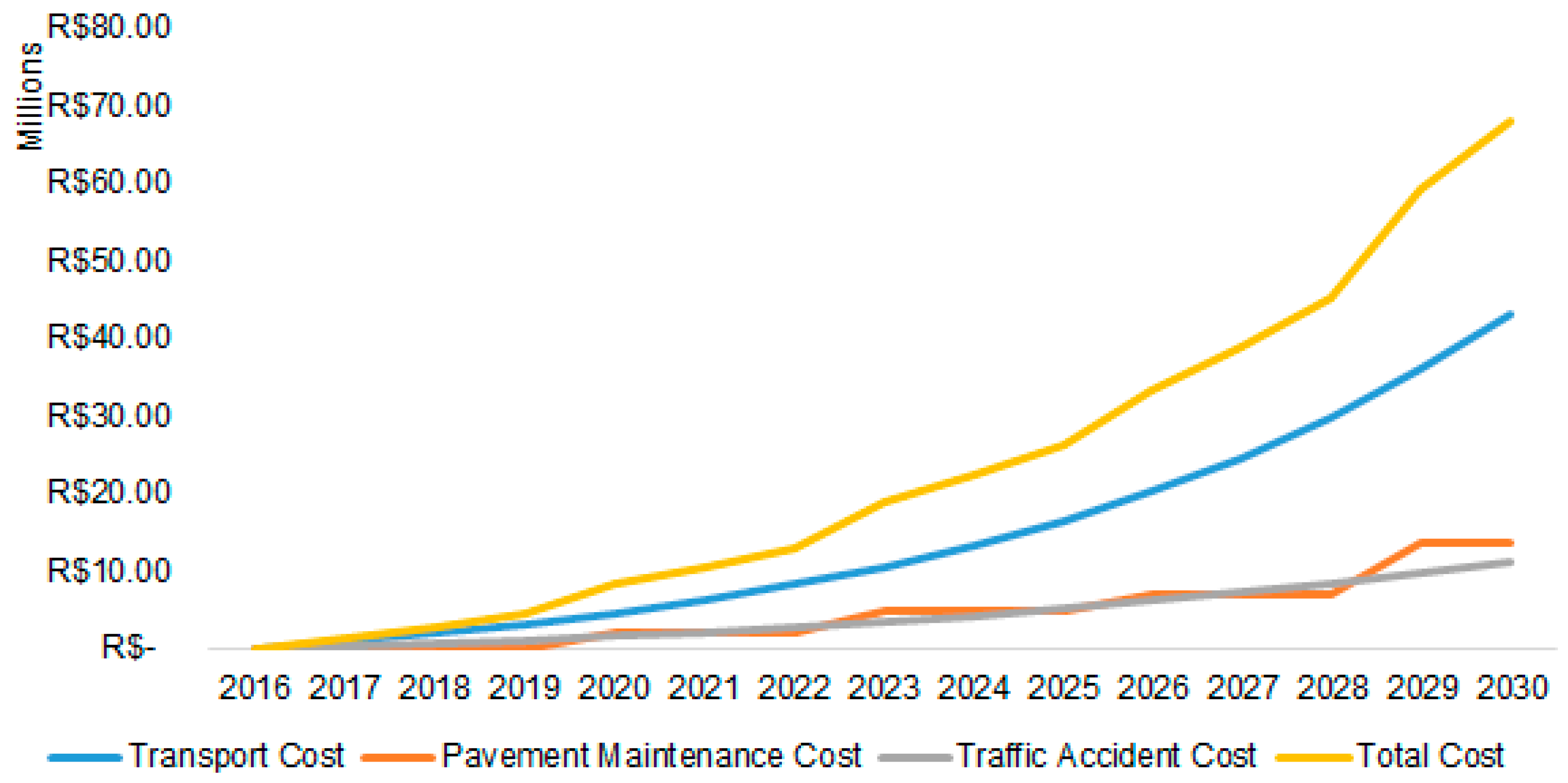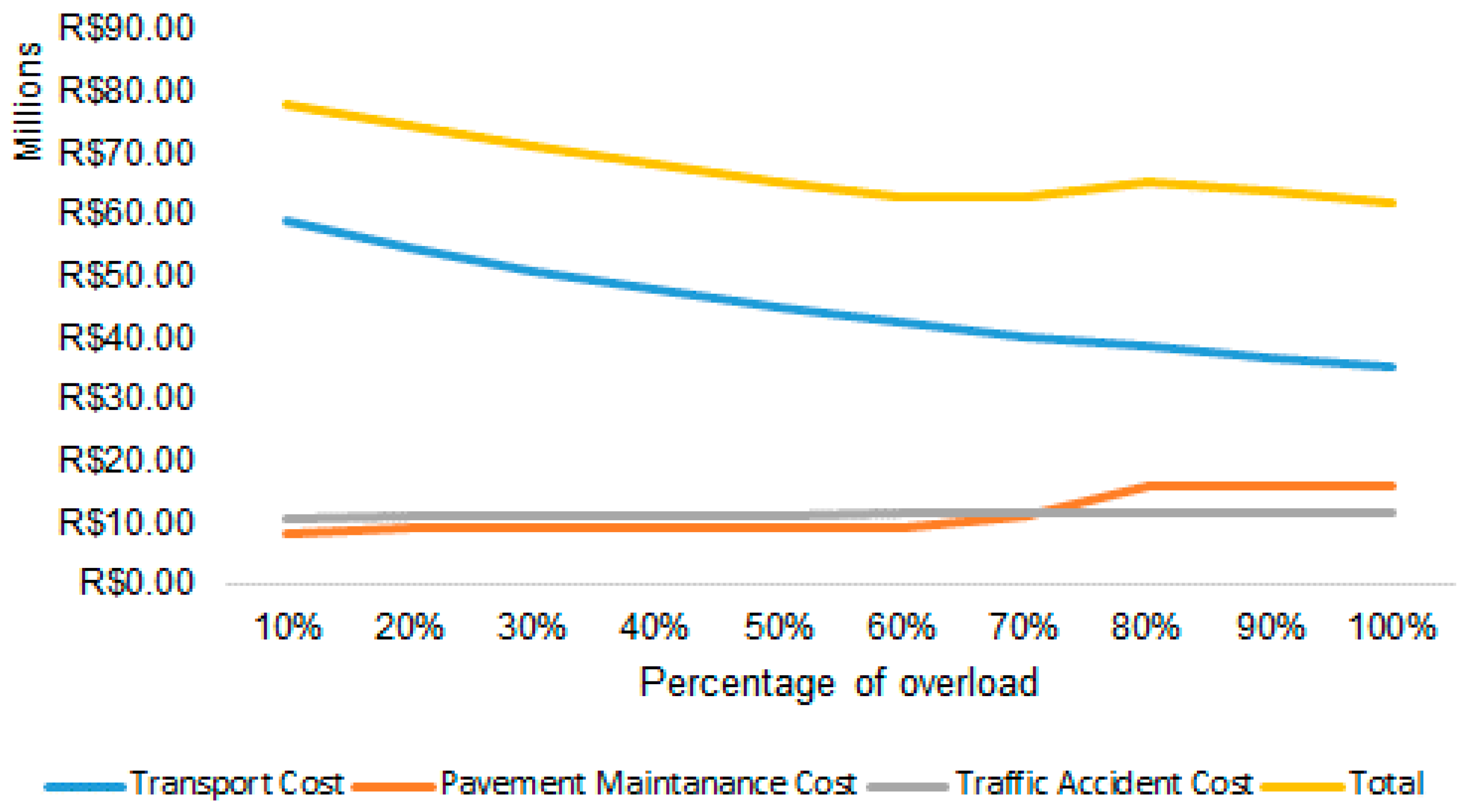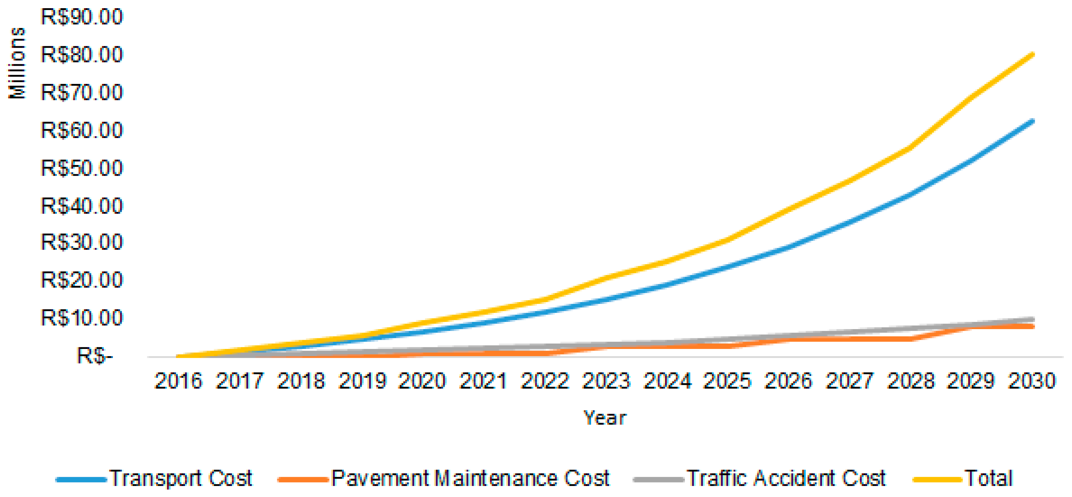Figure 14 shows the cumulative costs with transportation (operational cost), pavement maintenance and traffic accidents (social costs), as well as the total costs for the Reference Scenario.

It can be seen that the operational cost with transportation is more expressive than the sum of social costs with pavement maintenance and traffic accidents, representing 63% of the cumulative total costs in the period between 2016 and 2030. Nevertheless, it is worth highlighting that social costs are undersized, since only pavement maintenance and traffic accident costs were considered. Other important costs were not considered, among them, the delay of vehicle trips due to accidents and road blocks stands out, since it has several consequences for those involved, such as the need for companies to keep security stocks and the risk of degradation and environmental pollution with accidents involving vehicles with hazardous loads. The next scenarios show the impact of the percentage of overweight over system costs.

5.2. Strict, Moderate and Tolerant Policies

In the Strict Policy scenario, it was assumed that overload, both in TGW and on axles, is null, that is, the legal weight limits would be followed by freight carriers. In this case, the costs are shown in Figure 15.

The legal imposition regarding weight limits in freight vehicle loading increases the operational cost of transportation, once this cost is subdivided by the load transported, preventing the economy of scale achieved with overloading. Thus, despite the legal load limit of the vehicle is respected, the operational cost of transportation increases because a larger number of vehicles are required to carry the load.

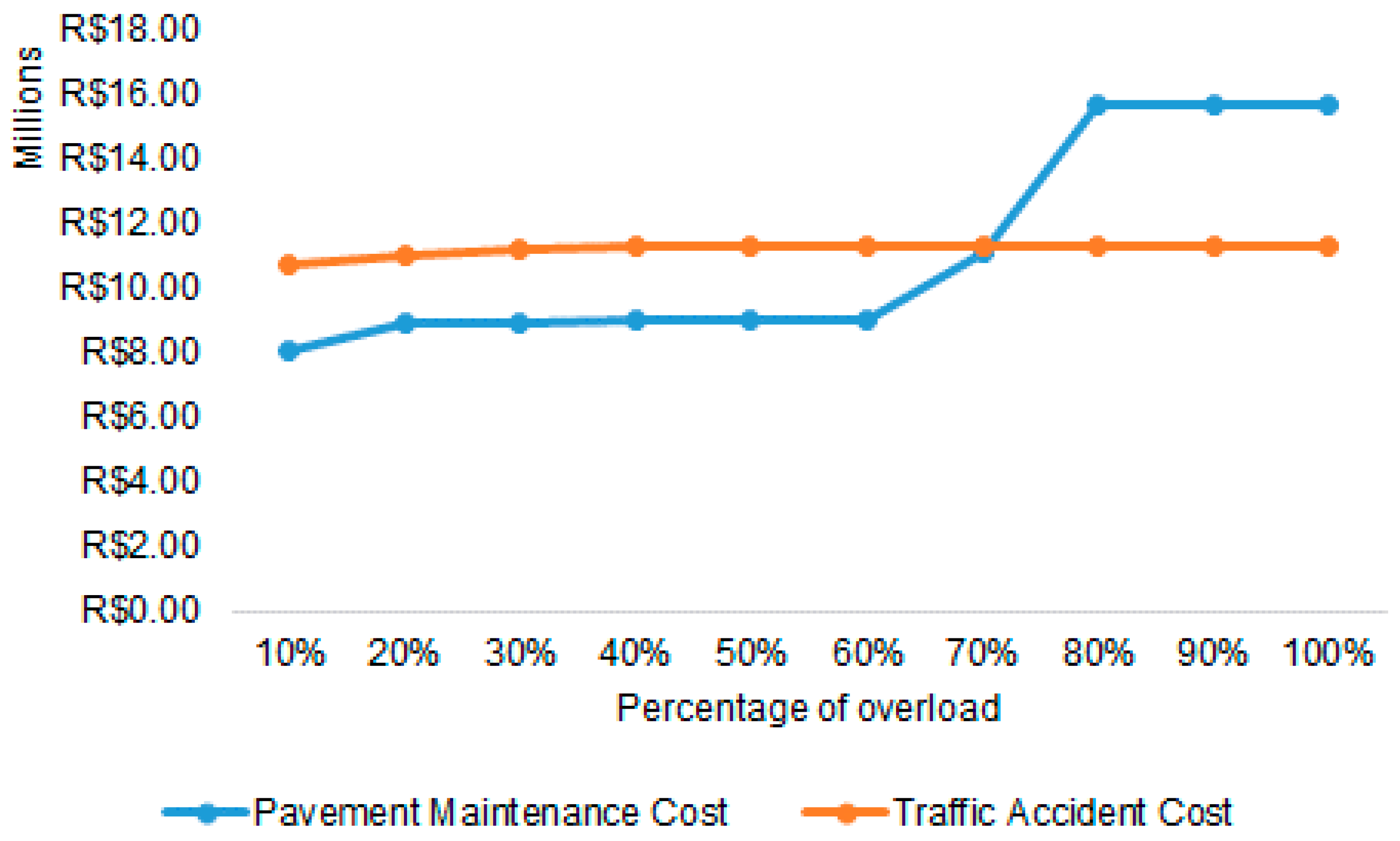
On the other hand, social costs with maintenance and accidents are reduced in relation to the Reference Scenario, as shown in Figure 16. In the maintenance of the pavement, the reduction of costs occurs in this scenario because, despite the increase in the number of axles passages, due to the increase in the number of trips, it can be concluded that the weight of the axles is more relevant in the deterioration of the roads. Likewise, accidents are influenced by the number of vehicles traveling on the highway, by the excess weight and by the traffic conditions of the highways, which are reduced by the practice of overweighed vehicles.

The operational cost with transportation increases by 45%, costs with maintenance and traffic accidents reduce by 41% and 12%, respectively and total cost increases by 18%. It is worth highlighting that studies should be carried out aiming to measure the number of accidents caused exclusively by the vehicles that transport ornamental stones, considering that the number of accidents in the model is estimated by the percentage of volume of these vehicles and the total number of accidents in the road, without differentiation of the type of vehicle involved. Moreover, it is also necessary to attribute then importance to each type of cost in order to decide on the best scenario.

In the Moderate Policy, the percentage of overload varies from 10% to 50% and in the Tolerant Policy, it varies from 60% to 100%. In this scenario overweight was gradually increased, from 10% to 100%, in order to separately assess the behavior of each cost and the total system cost, as shown in Figure 17.

The costs presented regard the cumulative cost at the end of the simulation period, that is, they are the total costs between 2016 and 2030. It can be seen that, as the overweight percentage increases, the operational cost of transportation decreases, that is, the unitary cost per tons of load carried, which confirms the economy of scale achieved by the practice of overweight in transportation. The minimum transportation cost occurs with an overweight percentage of 100%.

On the other hand, the minimum social costs happen with an overweight percentage of 10% (but they are even lower under the Strict Policy) and increase as overweight increases, as shown in Figure 18.

While the reduction in total system cost may reach 23% between the Strict Policy and the Tolerant Policy, the variation in social costs with the increase in overweight is not so significant. In the case of pavement maintenance costs, that happens because there are limiting factors to carry out maintenance works, such as the limits of pavement condition [61] in function of the IRI, the time intervals between the survey of such conditions, which may take from two to five years, as well as the duration of maintenance works, that is, the maintenance cost increases within these limits and not exclusively in function of the overweight being practiced.

Therefore, although pavement performance decreases as the overweight practiced by the transportation of ornamental stones increases, an overweight of up to 60% only in these vehicles would not lead to a significant increase in maintenance costs, considering the limiting factors presented and the case study in which only ornamental stone vehicles travel with excess weight, that is, the excess weight of the other freight vehicles that travel along the road was not assessed in this study. In the case of traffic accidents, deeper studies should be carried out regarding the occurrence of accidents and the cause exclusively related to overweight in ornamental stone vehicles.

However, decision makers must consider the importance of each cost category for society. Therefore, the next scenario assesses the costs based both on the variation in overweight and on the importance of social costs in relation to the operational cost of transportation.

5.3. Assessment of the Best Policy

The variation in the relative importance of the social cost in relation to the operational cost must be considered by decision makers as a criterion to assess the best policies to be adopted based on the minimization of total costs.

Table 13. Cumulative total cost considering a variation in overweight percentage and the importance of social cost in relation to the operational cost (R$ millions).

Importance of Social Cost		Not Important			Little Important		Equally Important	Very Important		Extremely Important
Weight of social cost		0	10	20	30	40	50	60	70	80	90	100
Strict Policy	0%	62.4	58.0	53.6	49.1	44.7	40.2	35.8	31.4	26.9	22.5	18.0
Moderate Policy	10%	58.9	54.9	50.8	46.9	42.8	38.9	34.8	30.8	26.8	22.8	18.8
	20%	54.6	51.2	47.7	44.2	40.7	37.3	33.8	30.4	26.9	23.4	19.9
	30%	50.9	47.8	44.8	41.7	38.6	35.5	32.5	29.4	26.3	23.2	20.1
	40%	47.6	44.9	42.2	39.5	36.7	34.0	31.2	28.5	25.8	23.0	20.3
	50%	44.8	42.4	39.9	37.5	35.0	32.6	30.1	27.7	25.2	22.8	20.3
Tolerant Policy	60%	42.4	40.2	38.0	35.8	33.6	31.4	29.2	27.0	24.8	22.5	20.3
	70%	40.3	38.5	36.7	34.9	33.1	31.4	29.6	27.8	26.0	24.2	22.5
	80%	38.4	37.3	36.1	35.0	33.8	32.7	31.6	30.4	29.3	28.2	27.0
	90%	36.6	35.7	34.7	33.7	32.8	31.8	30.9	29.9	28.9	28.0	27.0
	100%	35.0	34.2	33.4	32.6	31.8	31.0	30.2	29.4	28.6	27.8	27.0

Note: The highlighted cells indicate the lowest values of the respective columns.

shows total system costs, considering the importance of social cost, ranging from 0 (not important) to 100 (extremely important) for each loading policy (strict, moderate and tolerant).

The results in Table 13 show that, for the case in which social costs have lower importance than the operational cost or they are equally important, the best alternative is 100% overweight to reduce the system’s total cost. For a relative importance of social costs ranging from 60% to 80%, total costs are minimum with freight vehicles being 60% overweighed. Only in the scenario in which social costs are extremely important in comparison to the operational costs, the minimum total cost is identified in the strict policy, in which the legal weight limits are respected.

It is up to decision makers, again, to attribute due importance to each analyzed cost category. Nevertheless, considering that pavement deterioration in the analyzed road links affects the country’s logistics infrastructure and the competitiveness of the national production and that costs with accidents are assumed to be null in an ideal scenario, social costs should be considered extremely important to the interests of the society as a whole and not only to a reduced group of private companies.

5.4. Overweight in All Routes

The purpose of this scenario is to assess again the behavior of the costs considered in the model under the condition of overweight being practiced in all possible routes used to transport ornamental stones production, regardless of the existence of scales and their use for inspection and considering the absence of a toll station in Route #1.

This scenario is likely to occur in practice because, despite the existence of the weighing scale on Route #2, it does not work all the time. For that, the variable “Overload Percentage” was added to vehicle loading in Route #2.

Table 14. Costs in the scenario in which all routes have overloading (R$).

Scenario	Overweight	Cost of Transportation	Cost of Pavement Maintenance	Cost of Traffic Accidents	Total
Strict Policy	0%	62,444,356.00	8,072,306.00	9,956,531.00	80,473,193.00
Moderate Policy	10%	56,880,892.00	6,418,579.00	9,999,498.00	73,298,969.00
	20%	51,983,908.00	6,862,883.50	9,936,235.00	68,783,026.50
	30%	48,008,948.00	6,113,306.50	9,944,422.00	64,066,676.50
	40%	44,772,580.00	7,871,248.50	10,003,806.00	62,647,634.50
	50%	41,712,944.00	8,553,867.00	9,969,701.00	60,236,512.00
Tolerant Policy	60%	39,496,832.00	8,552,256.00	10,067,161.00	58,116,249.00
	70%	37,418,580.00	11,413,970.00	10,135,188.00	58,967,738.00
	80%	35,393,508.00	16,106,194.00	10,125,914.00	61,625,616.00
	90%	33,539,002.00	16,100,504.00	10,124,556.00	59,764,062.00
	100%	31,890,532.00	16,098,772.00	10,132,575.00	58,121,879.00

Note: the highlighted cells indicate the lowest values of the respective columns.

shows the operational costs with transportation, pavement maintenance and traffic accidents, as well as the cumulative total cost for each percentage of overweight practiced in both possible routes for the transportation of ornamental stones.

As the overweight percentage equally increases in both routes, there is a more equalized proportion of distributed load volume and, different than what happened in the previous scenarios, the costs with pavement maintenance and traffic accidents initially decrease, since these impacts do not overload only one route. Next, with 30% and 20% of overweight, maintenance and accident costs increase, respectively.

Total cost is still minimized under the Tolerant Policy, with an overweight of 60% per vehicle, since the operational cost is more expressive than the social costs, in case the relative importance of each cost is not considered.

The relative importance of social costs in relation to the operational cost was also simulated for the case in which both routes have overweighed ornamental stones vehicles. The results once again show that, the higher the importance of social costs due to pavement maintenance and traffic accidents in relation to the operational cost of transportation, the lower the percentage of overweight should be in order to minimize total costs.

The difference in costs between the scenarios with overweighting only in Route #1 and with overweighting in Routes #1 and #2 varies from 6% to 15% according to the weight of the social cost, that is, economically it is better for the overweighed ornamental stone vehicles to use two routes instead of only one, since the damage caused by overweight in only one route is higher for the system under the established conditions.

That happens because, with overweighed ornamental stone vehicles only in Route #1, the proportion of load volume in this route is in average 90%, causing most ornamental stone vehicles to use this route, thus punishing it in relation to Route #2. Now if overweighting is practiced in both routes, the proportion of load volume in Route #1 drops to 48% in average, therefore balancing the damage caused by overweight in both routes. Nevertheless, it is known that, in practice, freight vehicles choose Route #1 due to its lower operational cost and due to the absence of tolls and that overweighed vehicles also choose this route due to the absence of scales and the lower probability of inspections in comparison to Route #2.

6. Conclusions

This study presented an SD model that enables the assessment of the relationship between overweight in road transportation of ornamental stones and the costs associated with the operational cost of transportation and to social costs due to traffic accidents and pavement maintenance. Moreover, weights were attributed to the operational and social costs to assess the best policies in each case.

A literature review was carried out and showed some limitations, such as the consideration of a roadway dedicated to the transportation of a specific load; this view simplifies the problem in relation to reality, since it does not consider the traffic of other vehicles and its impacts on important variables such as road capacity, travel time and operational cost of transportation.

The model proposed regarding the case study showed the importance of observing the time interval between the assessments of pavement conditions and the duration of maintenance works, which significantly impact pavement maintenance cost. However, these time intervals do not take into consideration the delay between making a decision about the need for maintenance and the effective beginning of road works, including biddings and the hiring of third-party providers to carry out the maintenance service. This delay may further affect the pavement performance indicator, so it is valid to analyze, in the future, the impact caused by this delay.

The results confirm the advantage of the entrepreneurial strategy of overweighting ornamental stones transportation vehicles to reduce the unit operational cost of transportation. Nevertheless, as the overweight percentage increases, the social costs involved also increase. This way, there is a trade-off between the reduction of operational cost and social costs and they must be measured according to their respective attributed importance.

The practice of overweighting per axle increases productivity and profit in the transportation industry, since it decreases the unitary transport cost per tons of load; on the other hand, it brings disadvantages to society, such as the fast deterioration of pavements, an increase in road maintenance costs and reduced road safety due to the increase in accident rates, as seen in the analysis performed in this study.

Despite the scenario with 100% overweight was hypothetical for simulation purposes, we note that there were already registrations of up to 70% in groups of axles and up to 57% in TGW of ornamental stones vehicles. This implies in reducing road safety and other studies are recommended for a deeper analysis of these conditions.

Also, a more detailed cost-benefit analysis is indicated because the use of overweighed vehicles reduces the number of trips but increase the unitary costs of the trips (generalized costs) due the lower average speed and fine costs, for example. Moreover, the overweighed vehicles need more maintenance due to the accelerated wear of the vehicle parts but the fleet used is smaller and therefore the number of maintenances is also smaller [21]. This kind of analysis was not carried out in this study due to lack of available data but it is also indicated for future researches.

The deterioration of Brazilian highways has a direct impact on logistics costs and, consequently, on the competitiveness of national products in a globalized economy. Furthermore, the lack or low quality of infrastructure discourages new investments. Regarding traffic accidents, this study only uses measurable costs, that is, the costs of accidents analyzed here are underestimated, since no studies have been found that consider the cost with the loss of lives, for example. The literature mentions the difficulty of measuring the loss of lives beyond the economic loss. Besides, it was not possible to find data that attempted to estimate or suggest a value to this loss.

Also, there are other costs associated with these negative externalities that were not measured in this study, such as indirect costs related to trip delays in the occasions in which the road are blocked due to accidents, leading companies to keep safety stocks (even those companies that depend on daily supply of inputs) and the personal losses of various road users. Other costs that were not measured in this study regard environmental impacts caused when these accidents involve vehicles transporting hazardous materials, risking the environmental integrity of the ecosystem around the event. Therefore, social impacts should be better studied and measured for a more precise assessment of the real costs involved.

For the scenario in which social costs are deemed extremely important, results show that a strict policy should be adopted regarding the tolerance of overweighting in carrier vehicles. However, an ever higher legally admitted tolerance has been identified in Brazil regarding the weight transmitted per axle, which contributes to the accelerated deterioration of pavements and other associated damage. Even so, violations of weight limits are frequent on national roadways. That is why it is necessary to invest in more efficient policies and actions such as uninterrupted inspection, driver awareness, mandatory declaration of freight weight in the invoice and fines equivalent to the profit achieved through the practice of overweighting.

In this context, this study contributes to the literature in that it attempts to complement the knowledge in the area, supporting strategic planning and decision making concerning the development and implementation of policies that regulate freight transportation in the Brazilian road transportation system, assisting in the understanding of the system’s behavior, in the quantification of the costs involved based on the percentage of overweighting being practiced but especially on the importance attributed to each cost category.

Within the same scope, some factors may be analyzed in more detail if addressed by new studies. Examples of that would be: the inclusion of a module considering the environmental impacts caused by the practice of overweighting in freight vehicles, such as increased fuel consumption, costs with air pollutant and greenhouse gas emissions; the analysis of other social impacts for a better estimate of the actual costs indirectly incurred by the society due to the practice of overweighting; the inclusion of other vehicle categories with overweighting that travel along the analyzed route; and the comparison of costs in a scenario of logistic integration with the use of more efficient modes of transportation, such as railways and waterways.

The proposed model contributes to the understanding of the dynamic behavior of the ornamental stones transportation system under different vehicle loading policies, with results that support decision making in favor of sustainability in transportation.