Article

On the Unsustainable Macroeconomy with Increasing Inequality of Firms Induced by Excessive Liquidity

1
Graduate School of Frontier Sciences, The University of Tokyo, Chiba 277-8563, Japan
2
Advanced Science Research Laboratory, Saitama Institute of Technology, Saitama 369-0293, Japan
*
Author to whom correspondence should be addressed.
Current address: Room 216, Environmental Building, Kashiwanoha 5-1-5, Chiba 277-8563, Japan.
Sustainability 2019, 11(11), 3075; https://doi.org/10.3390/su11113075
Submission received: 23 April 2019 / Revised: 27 May 2019 / Accepted: 28 May 2019 / Published: 31 May 2019
(This article belongs to the Section Economic and Business Aspects of Sustainability)

Abstract

:
This research studies how excessive liquidity can trigger catastrophic economic crises in a stylized macroeconomic agent-based model (ABM). Previous studies showed the relevance of the income distribution to the economic crises, whereas we find, in a well-studied macroeconomic ABM endowed with diverse economic performance of firms, while providing moderate liquidity serves as an effective tool to stabilize the economy, excessive liquidity may cause abnormal dispersion of firm’s wealth and the subsequent severe endogenous crises. The mechanism for such large-scale crises is found in the model as the increasing gap of financial fagility between the advantageous and disadvantageous groups of firms. Two factors, diverse production cycles and variable wages, are used to explore the robustness of the occurrence of crises. Moreover, our study shows that the leverage ratio based on aggregate values may underestimate the systemic risk. Hence, a proposal for the new design of the risk measurement in the macro-economy and insights into monetary policies for a sustainable economic development is given.

1. Introduction

Thanks to the tremendous progresses in science and technology, we have witnessed a trend of worldwide economic growth with expanding population and capitalization in the past decades. Nowadays, achieving sustainable economic prosperity has become one of the most concerned issues for many developed and developing countries. The sustainability of an economy needs harmonious coevolution of economic, social and environmental systems [1,2]. Some occasional GDP declines in the growth trend, normally regarded as indications of the system being in the contractions phases of business cycles, may bring the opportunities for cultivating the technology innovations that better promote sustainability [3,4]. Nevertheless, other rare ones, accompanied by widespread bankruptcies of firms and banks, indeed impose devastating effects on the economic systems, causing long-term unrest in all aspects of society. Some prominent examples are the Great Depression in 1929 and the Japan’s collapse of bubble followed by a Lost Decade in late 1980s. These macroeconomic catastrophies lead not only to a large-scale of individual tragedies but also to an impaired financial capacity of a country to an extent where the sustainable coordination among subsystems of the society and the nature becomes unaffordable [4,5]. Therefore, understanding the mechanisms underlying such huge economic crises and preventing them are significant to the sustainability of an economy.
In line with previous emperical studies, the economic crisis can be ascribed to many causes, such as misusing and overusing of leverage, speculation bubbles, contagion effect, etc. Among those, the rapid increase in inequality of households’ income before 1929 and 2007 is found closely related to the subsequent great crises [6,7,8,9]. However, in fact, typical sources of income, such as wage, bonus and dividend, are highly related to the relevant company’s abilities of making profit and generating cash flow. Thus, the observed income inequality may also reflect an increasing gap of the financial status between the advantegeous firms or sectors attracting inflows of capitals, and the disadvantageous ones whose operation may overly rely on debts. For instance, before the subprime crisis in 2007, while the bankers who were doing business related to subprime loans received huge bonuses, the financial and real estate sector also became the largest share in S&P 500 by market value, showing very strong profitability of the firms in this sector at that time. Nowadays, the most attractive firms to capitals seem to be the internet giants, named as FAANG (the best-performing U.S. tech stocks, namely Facebook, Apple, Amazon, Netflix and Alphabet’s Google) by Wall Street. Difference in financial status of firms can simply originate from the characteristics of relevant sectors, for instance, manufacturing firms in need of high capital investment usually have high financial leverages but some Internet firms which have rapidly growing cash flows may have very low financial leverage. Thus, considering the many fundamental differences among firms, "heterogeneity" is hereafter used to term the large variance in the firms’ economic performance.
Despite being plausible, the causality between this heterogeneity of firms and the emergence of a large wave of firm bankruptcy has yet to be established on a theoretical basis due to the complexities involved in an economic system. We hence are motivated to set up a preliminary framework for studying the relationship between heterongeneity of firms and severe economic crisis in this research. As opposed to directly reaching some mathematical equations, a feasible starting point could be first investigating this problem in simulation experiments and to draw implications in a qualitative sense. Among the different kinds of models for macroeconomic system, a well-studied agent-based model (ABM), the Mark0 model propsed by Gualdi, et al. [10], is chosen because of its controlled complexity and the flexibility for model extensions in the most straightforward way. Mark0 is a closed-system economy consisting of two sectors, firms and households, competing for a conserved amount of money through the supply and the demand of products. It can exhibit several different equilibrium states of economy including the one with endogenous crisis due to insufficient monetary easing. We design a new model called HoP-Mark0, where the heterogeneity of firms’ performance is ingegrated into Mark0, and find in HoP-Mark0 that a new type of catastrophic endogenous crisis featuring enhanced bankruptcy and unemployment emerges if too much liquidity is given. The origin of this interesting phenomenon is examined thoroughly from the statistics of leverages of individual firms.
The outline of this paper is as follows: Section 2 provides an overview of theoretical background of some related models for macroeconomy; Section 3 gives a brief introduction to the assumptions, features and results of Mark0; In Section 4, we demonstrate our modification of the integration of firm heterogeneity into Mark0 and show the results; In Section 5, we discuss the robustness of results with some model extensions of diverse production cycles and variable wages; In Section 6, we draw some implications on the measurement of risk of the severe economic crisis. Section 7 concludes this article with reflections on model limitations and some future tasks.

2. Theoretical Background

The mainstream macroeconomic models used by central banks and governments are the dynamic stochastic general equilibrium (DSGE) models. Based on a set of differential equations describing dynamic relations among many macroeconomic measures under appropriate assumptions, standard DSGE models excel in quantitative prediction of macroeconomic measures for systems in business cycles or economic growth but perfrom poorly at out-of-equilibrium phenomena such as economic bubbles and crisis [11,12,13,14,15]. In standard DSGE models, a severe economic crisis can only be triggered by a large exogenous shock [16,17,18] rather than endogenously occur, while in reality, it seems that large shocks are the result of an economic crisis. Moreover, each sector of DSGE-modeled economy is described as a representative agent, for instance, firms or households, whose behaviors are formulated by a set of ordinary differential equations based on the economic rationale. Such practice of modeling implicitly assume that the aggregation of multiple firms or households should be equivalent to the corresponding representative agents, which is justifiable only if the interactions among the group of agents are weak enough and meanwhile, the rationality of the agents’ behavior must be perfectly ensured. However, during the periods of bubbles and crises, the interactions among agents could be significantly enhanced by the contagion effect and the rationality in decision making could be distorted due to the herding behavior [14,15,19].In past decades, many sophisticated modifications has been made to improve DSGE models in these two aspects [20,21,22] to strengthen their quantitative credibility for better policy-making.
However, to meet our research purpose of qualitative exploration on the relationship between increasing gap between firm financial status and endogenous crisis, using ABMs featured by interacting individuals [18,23] would be more feasible. The agent-based approach has been extensively used in physical, chemical, biological and social systems [24,25,26,27,28,29] to understand unexpected phenomena emerging from a group of heterogeneous and adaptive interacting agents. As a set of powerful tools in linking micro-behaviors to macro-phenomena in a class of complex adaptive systems, agent-based modeling and simulation have also been applied to the analyses of macroeconomic phenomena [10,23,30,31,32,33,34,35,36,37,38]. Generally, we can differentiate the previous ABM studies into two categories. In the first genre, ambitious researchers are building the full-scale ABMs which includes as many different types of economic agents and their complicated interactions as possible. A famous example of the full-scale models is EURACE [32,33], which is designed to recover various economic processes and to provide a platform for testing policies for decision-makers. However, the huge number of degrees of freedom caused by many behavior rules, initial conditions and other parameter settings in the model makes the verification of the robustness of results very hard. In the second genre, researchers are making efforts to build the minimal ABM by keeping only the least number of types of agents and employing highly abstract models of the interactions [36,37,38]. Although the full range of phenomena occurring in a real economy can hardly be reproduced with the minimal ABMs, the link between microscopic mechanisms and some specific macroscopic phenomena can be elucidated more easily. In this sense, the minimal ABMs work as spin models [39,40] do in statistical physics to reveal basic conditions and control parameters for a spectrum of phenomena, such as criticality, phase transitions, relaxation behaviors, etc. [41,42], instead of an instance that reproduces the real economy in all details. Indeed, the development of minimal ABMs for financial markets, such as Minority Game [43,44], Cont-Bouchaud model [45], and V. Alfi’s model [46,47], etc., has been one of the focused topics in econophysics, a new research field advocated by the famous physicist E.G. Stanley et al. [48] since the late 90s.
The Mark0 version of CRISIS model is a typical minimal macroeconomic model [10], which consists of only two sectors, namely, firm and household, competing for a conserved pool of total wealth. Firms are further modeled as multiple interacting agents, while the household sector is kept as a representative agent. The government and the central bank are functioned by environmental parameters. Nevertheless, even with only the supply-side played by interacting agents with basic heuristic behavioral rules, it is enough for such a model to give unexpected but reasonable pictures of economic circulations with endogenous crisis. In the study of Mark0, constructing the phase diagram is essential to illustrate different economic status controlled by a couple of key parameters. In Mark0 economy, the level of liquidity is found to be very crucial to separate distinct phases, namely the residual unemployment (RE) phase (low liquidity level), the endogenous crisis (EC) phase (medium liquidity level) and the full employment (FE) phase (high liquidity level). In another study on Mark0 [49], the authors further simplified the model and found that the occurrence of endogenous crises could be explained by the synchronization of interacting oscillators. The simplicity of Mark0 renders it into an ideal framework where model extensions could be easily made and its results into a benchmark for understanding complicated results from sophisticated extensions of interest. Hence, we chose it as a basis on which our exploration could be performed.

3. A Brief Review of Mark0

Mark0 is kept simple to study the basic economic circulation between the demand and the supply of products [10,37]. Hence only two kinds of agents, household and firm, are involved. The basic framework of Mark0 can be described as three flows of money (Figure 1): (1) From the households to the firms, i.e., the households pay for the goods produced by the firms; (2) From the firms to the households, i.e., the firms pay wage and dividend to households; (3) From the household and firms with positive cash balance to the other firms, i.e., the household and healthy firms pay the funds for offsetting the bad debts of bankrupt firms and the funds for starting new firms. The total amount of money M, which is the sum of firms’ net equity and households’ wealth, is conserved in the circulation:
i = 1 N f max [ 0 , ε i ( t ) ] + i = 1 N f min [ 0 , ε i ( t ) ) ] + H ( t ) M
where N f is the total number of firms, ε i ( t ) is the cash balance of each firm and H ( t ) is the households’ wealth. A positive value of ε i ( t ) indicates that firm i holds cash, whereas a negative value of ε i ( t ) indicates that firm i has debt. Hence i = 1 N f max [ 0 , ε i ( t ) ] and i = 1 N f min [ 0 , ε i ( t ) ) ] indicates the total amount of the firms’ asset and debt, respectively.

3.1. Firm

A firm and its product are tagged with an index i = 1 , 2 , N f . The state of firm i is described by price p i ( t ) and production Y i ( t ) of its product, wage w i ( t ) for a unit of labor force and cash balance ε i ( t ) . A firm needs to decide how many products to be produced and how much the price of each product to be sold, considering with both the firm’s internal status (costs, liabilities, capacity, etc.) and the market conditions (demand for its products, supply of the materials, competition, etc.). The firm in Mark0 adopts a set of heuristic rules to adapt with the constantly changing competitive environment. Firm i would adjust the production Y i ( t ) to match the market demand D i ( t ) for its product and adjust the product price p i ( t ) based on the average price p ¯ ( t ) in order to compete with the other firms. Updating rules for the two variables are listed as follows:
if Y i ( t ) < D i ( t ) : Y i ( t + 1 ) = Y i ( t ) + min { η + [ D i ( t ) Y i ( t ) ] , μ u ˜ i ( t ) } , if p i ( t ) < p ¯ ( t ) : p i ( t + 1 ) = p i ( t ) [ 1 + γ p ξ i ( t ) ] ; if p i ( t ) p ¯ ( t ) : p i ( t + 1 ) = p i ( t ) ; if Y i ( t ) D i ( t ) : Y i ( t + 1 ) = Y i ( t ) + max { η [ D i ( t ) Y i ( t ) ] , 0 } , if p i ( t ) p ¯ ( t ) : p i ( t + 1 ) = p i ( t ) ; if p i ( t ) > p ¯ ( t ) : p i ( t + 1 ) = p i ( t ) [ 1 γ p ξ i ( t ) ] .
where p ¯ ( t ) = i p i ( t ) Y i ( t ) i Y i ( t ) is the production-weighted average of price over all firms at time t; ξ i ( t ) are random numbers from a uniform distribution U(0,1) (which are independent across firms and across time steps); γ p , η and η + are parameters to control the magnitudes of price and production adjustments. The upward adjustment of production is limited by the maximal available labor force, μ u ˜ i ( t ) , which is calculated as
μ u ˜ i ( t ) = e β w i ( t ) / w ¯ ( t ) i e β w i ( t ) / w ¯ ( t ) μ N f u ( t ) ,
where w ¯ ( t ) = i w i ( t ) Y i ( t ) i Y i ( t ) is the production-weighted average of wage over all firms and u ( t ) = 1 i = 1 N f L i ( t ) μ N f is the unemployment rate at time t. Note that μ N f is the total number of labor force provided by the household sector and L i ( t ) is the amount of labor employed by firm i. Because μ has little influence on the main results of Mark0, μ is set to 1 for simplicity.
After adjusting price and production in one round, each firm would update its cash balance. The only cost of production is the wage paid by the firm. Mark0 adopts a simple linear production function, Y i ( t ) = λ L i ( t ) , where λ is the technological parameter. For simplicity, both λ and the wage w i ( t ) remain constant and are set to one in the simulation. Therefore, the cost of production equals to L i ( t ) w i ( t ) and the currently realized profit ρ i ( t ) :
ρ i ( t ) = p i ( t ) min [ Y i ( t ) , D i ( t ) ] L i ( t ) w i ( t ) = p i ( t ) min [ Y i ( t ) , D i ( t ) ] Y i ( t ) .
If both ρ i ( t ) and ε i ( t ) is positive, firm i will pay dividend, δ ρ i ( t ) to the household. The cash balance will be updated as:
ε i ( t + 1 ) = ε i ( t ) + ρ i ( t ) δ ρ i ( t ) θ δ ρ i ( t ) ) ,
where θ ( x ) is the Heaviside step function, θ ( x 0 ) = 1 and θ ( x < 0 ) = 0 . If the cash ε i ( t ) is not enough for the cost of production L i ( t ) w i ( t ) , the firm can get loan from the bank and ε i ( t ) could be a negative value when firm i is in debt. The financial fragility is measured as the negative of the ratio of the cash balance over the payroll,
Φ i ( t ) = ε i ( t ) Y i ( t ) w i ( t ) .
Note that by its definition, Φ i can also be interpreted as the leverage of an individual firm. The indebtment level of a firm would be limited by a default threshold θ . Firm i would be allowed to continue operating as long as Φ i ( t ) is less than θ . When Φ i ( t ) θ , the overindebted firm will go bankrupt. Thus, the parameter θ is similar to a money multiplier and controls the credit creation in the system. A larger θ means that the firms can obtain more liquidity with the same scale of operation.
The amount of bad debt of the firms would be added to a variable ε d which is the deficit to be borne by all the operating firms and the household, i.e., ε d ( t ) ε d ( t ) i B ( t ) min [ ε i ( t ) , 0 ] , where B ( t ) is the set of bankrupt firms at time t (the arrow “→” means “replaced by” hereafter). The bankrupt firm would become inactive temporarily and its debt would be cleared, i.e., ε i ( t ) 0 .
In each of the following simulation rounds, an inactive firm has a probability ψ to get revived. The necessary fund for revived firms, is another portion of ε d , which would be covered by the operating firms and the household as well, ε d ( t ) ε d ( t ) + j V ( t ) Y j ( t ) w j ( t ) , where V ( t ) is the set of revived firms at time t. The production Y j ( t ) and price p j ( t ) of the revived firms would be set as the available labor force μ u ˜ j ( t ) and the production-weighted average price p ¯ ( t ) , respectively. After all the firms have the operating status and the cash balances updated, ε d ( t ) would be deducted with priority from the households’ wealth, if H ( t ) ε d ( t ) :
H ( t + 1 ) = H ( t ) ε d ( t ) ,
and also from the accounts of the active firms with positive cash balance, if H ( t ) < ε d ( t ) :
H ( t + 1 ) = 0 , ε i ( t + 1 ) = ε i ( t ) H ( t ) ε i ( t ) ε d ( t ) H ( t ) i = 1 N f max [ ε i ( t ) , 0 ]
The cash flow is kept to be consistent so that the total money H ( t ) + i = 1 N f ε i ( t ) is conserved in the simulation, which guarantees Mark0 to to be a stock-flow consistency model as described in Equation (1).

3.2. Household

The state of the household sector is described by aggregate variables, namely the total saving H ( t ) , the total consumption budget C b ( t ) and the unemployment rate u ( t ) . In each round, the total saving is updated after the deduction of ε ( t ) (see Equations (7) and (8)) as following:
H ( t + 1 ) H ( t + 1 ) + i = 1 N f Y i ( t ) w i ( t ) + i δ ρ i ( t ) C ( t )
where i = 1 N f Y i ( t ) w i ( t ) is the total wage, i δ ρ i ( t ) is the dividend received, C ( t ) is the consumption expenditure. The total consumption budget C b ( t ) is a portion of the total wealth of household:
C b ( t ) = c H ( t ) + i = 1 N f Y i ( t ) w i ( t ) ,
where c is the propensity to consume products. The demand of product is then distributed among firms based on a submodel of choice making [50]:
D i ( t ) = C b ( t ) e β p i ( t ) / p ¯ ( t ) p i ( t ) Z ( t ) , with Z ( t ) = i e β p i ( t ) / p ¯ ( t ) .
Parameter β 0 determines the sensitivity of the households to the price. When β = 0 , the household agent would evenly distribute the consumption budget to all the products without any considerations of price. As β increases, the households become more sensitive so that the demand of product i will be strengthened if the price p i ( t ) is more competitive comparing with the average price p ¯ ( t ) . The demand D i ( t ) for the products of firm i would be limited by the realized production Y i ( t ) , therefore the actual consumption expenditure can be calculated as
C ( t ) = i = 1 N f p i ( t ) min [ Y i ( t ) , D i ( t ) ] .

3.3. Simulation Results and Phase Diagram

Here we would only give a short introduction of the simulation results of Mark0. The detailed analysis and discussion on the phase diagram of Mark0 can be found in [10]. Although there exist nine parameters in Mark0, it is found that the status of the model economy is controlled by only two parameters, the liquidity parameter θ and hiring/firing propensity R = η + / η which measures the ratio of amplitude of hiring and firing labor force. Note that R could simply be behavioral tendency of firms, or more sophisticatedly, could be induced by other mechanisms. According to a previous study [23,34], the asymmetry could result from the firms’ reactions to the changing of interest rates. The rest parameters could only have minor effects on the locations of the phase boundaries. The existence of the four phases, FU, RU, EC and FE, is quite robust against various modifications of the model [10,49]. The full phase space is split, by a critical hiring/firing propensity R c = 1 , into the region of FU and the regions of RU, EC and FE (Figure 2a). When R R c , the status of model economy is controlled by the liquidity parameter θ . In Figure 2b, we give the four typical time series of the unemployment rate in each of the four phases. When θ is very small, the economy would operate in RU phase and a medium value of unemployment rate persists; when θ is very large, the economy would operate in FE phase that almost all labor force in the model is employed, indicated by the nearly zero unemployment rates; when θ is set to an intermediate value, the EC phase emerges. When the model economy is operating in EC phase, the unemployment rate could be nearly zero most of the time as in the FE phase. However, the economic crises occur (quasi-)periodically, indicated by the sharp spikes of the unemployment. Although the other parameters could alter the amplitude and frequency of the crises, the occurrence of crises appear inevitable.
The global leverage ratio k, proposed in [10] can be used to help understand how the endogenous crises happen in the model economy:
k ( t ) = ε ( t ) H ( t ) + ε + ( t ) ,
where ε + = i max [ ε i ( t ) , 0 ] and ε = i min [ ε i ( t ) , 0 ] .
In a good state of the economy, the global leverage k gradually increases and stabilizes around a high level (Figure 3a), reflecting the firms’ demand for liquidity due to the expansion of production; on the other hand, in the case of a bad economy, k increases quickly at first but stabilizes around a relatively lower level, which is achieved by the balance between the surviving firms and the bankrupt firms. However, in the EC phase, the dynamics of the global leverage is characterized by recurring cycles of fast increase and sudden collapse corresponding to the occurrence of endogenous crises. This intermittent behavior is caused by the clustering of the indebted firms and will be discussed later in Section 4.4.
The results shown here are robust against the variation of other parameters. In [10], the authors have shown that different levels of N f almost make negligible difference to the dynamics and phase diagram, whereas varying γ p , c, β , δ , ϕ affects the fluctuation amplitude of unemployment rate and quantitatively changes the positions of phase boundaries. Also, many other factors such as interest rate, exchange rate, import/export ratio are not modeled because the research focus of Mark0 simulation is to pinpoint the internal variables governing the economy status and the emergence of crisis with a controlled complexity. The conclusion here regarding the critical role of liquidity in determining the phase of a closed-system economy (conserved total wealth with a stable population of households and a fixed pool of firms) can serve as a benchmark for further model extensions of interest to be compared with.
Based on the phase diagram of Mark0, we can infer that a regulator or a central bank only needs to implement a very loose monetary policy while keeping R > R c for achieving an eternally stable and low unemployment rate in an ideal closed system like the Mark0 economy. Moreover, the regulator should be very cautious when he/she tightens the liquidity because the phase transition from FE to EC is rather difficult to detect in the early stages. Nevertheless, as we will demonstrate in the following sections, even in a closed system, high liquidity may not always be a panacea if the firms have different financial status.

4. Heterogeneous Economic Performance of Firms

Firms can be very distinct from others in terms of economic performance. For firms operating in different sectors, the profit margins could be quite different because of sector-specific properties and different stage of development. In fact, even in the same industry, the gap of profitability could be huge between firms, due to a variety of complex causes, such as the ability of cost control and brand premium. For example, the net margins of Japan airlines and ANA group are 11.1% and 2.3% in 2014, respectively, although they were both large Japanese airlines.
Other factors which can cause profitability gaps among firms include market monopoly, difference in competitiveness (see Porter’s Five Forces Framework for analyzing firm’s competitiveness [51]), different costs of capital, etc.
In the original Mark0 model, the heterogeneity of firms’ economic performance was absent because firm agents adapt their price, production, and labor power to the demand of household by a set of homogeneous rules. No firm could be advantegeous over the others in a statistical sense. As a first step for the feasibility of qualitative analysis, we introduce diverse discount rates of price as a mean to express the heterogeneity of firms’ economic performance and study the influence on the phase diagram of the modeled economy. Note that the discount rate of price is just a measure of relative competitiveness which is an aggretate effect of the firm’s competence in multiple aspects such as product, management, sectors.

4.1. The Extended Model

Each firm agent would be endowed with a constant discount rate π i > 0 , which reflects the competitive advantage of the firm. Then the price p i in Equation (11) would be substituted by the modified price, p i ˜ = p i / π i .
With the modified price, consider that two firms with π i > π j , coincidentaly set their product prices the same, p i ( t ) = p j ( t ) . The demands for the products of firm i and firm j would be actually decided by p i ˜ ( t ) = p i ( t ) / π i and p j ˜ = p j ( t ) / π j ,which results in D i ( t ) > D j ( t ) . Hence firm i would have a higher probability than firm j to sell out its products. However, p i ( t ) and p j ( t ) would still be used in the transaction and accounting processes. Thus, firm i would have a higher profitability than firm j. From the perspective of the households, π i can also be regarded as a measure of the consumer preference to the product of firm i. In the following text, we will call the Mark0 model with the extension of heterogeneity of profitability as HoP-Mark0.

4.2. Result: Dynamics

Figure 4b shows the time evolution of the unemployment rate u ( t ) under different levels of liquidity θ and ratio R. The black curve (1—FU) corresponds to the situation R < R c , whereas the red (2—RU), light green (3—EC), blue (4—FE) and dark green (5—EC+) curves correspond to R > R c with increasing levels of liquidity θ . One can compare Figure 4b with Figure 2b and find that in HoP-Mark0, there exist a type severe endogeneous crisis (dark green) corresponding to very high liquidity, which could not be found in the Mark0 economy (Figure 2b). This type of crisis may deprive more households of their jobs than the endogenous crisis corresponding to medium liquidity (light green) can do. Similarly, Figure 3b shows the typical time series of the global leverage k ( t ) (Equation (13)) and one can easily spot a extremely large crash of k at time around 40000 steps (dark green) in HoP-Mark0 while this type of catastrophe is absent in the Mark0 economy (Figure 3a). Interested readers can refer to Appendix A for the time evolutions of all firms’ financial fragility (leverage of individual firms) Φ i ( t ) (Equation (6)) in Mark0 and HoP-Mark0, where huge difference should be identified between two types of endogeneous crises.

4.3. Result: Phase Diagram

Figure 4a gives the new phase diagram of HoP-Mark0 with five phases identified by their distinctive dynamics. In the phase diagrams of Mark0 (Figure 3a), FE phase persists for any increase in the default threshold θ , as long as θ is larger than the critical θ EC FE that separates EC phase. However, in HoP-Mark0 simulation, an additional phase, named endogenous crises plus (EC+), would emerge when θ is larger than a new critical θ FE EC + . The crises in EC+ phase is characterized by lower incidence but significantly larger amplitude of the burst. Moreover, the dynamics of unemployment rates in EC phase also becomes chaotic.
Hence, if considering the heterogeneity in firms’ economic performance, easy credit is no longer a panacea for the modeled economy. To achieve a low and stable unemployment, the available credit, controlled by θ , must be carefully set between the lower limit θ EC FE and the upper limit θ FE EC + . Otherwise, the modeled economy would suffer from frequently occurring crises when θ RU EC < θ < θ EC FE , or be in danger of extremely strong crises, when θ > θ FE EC + .

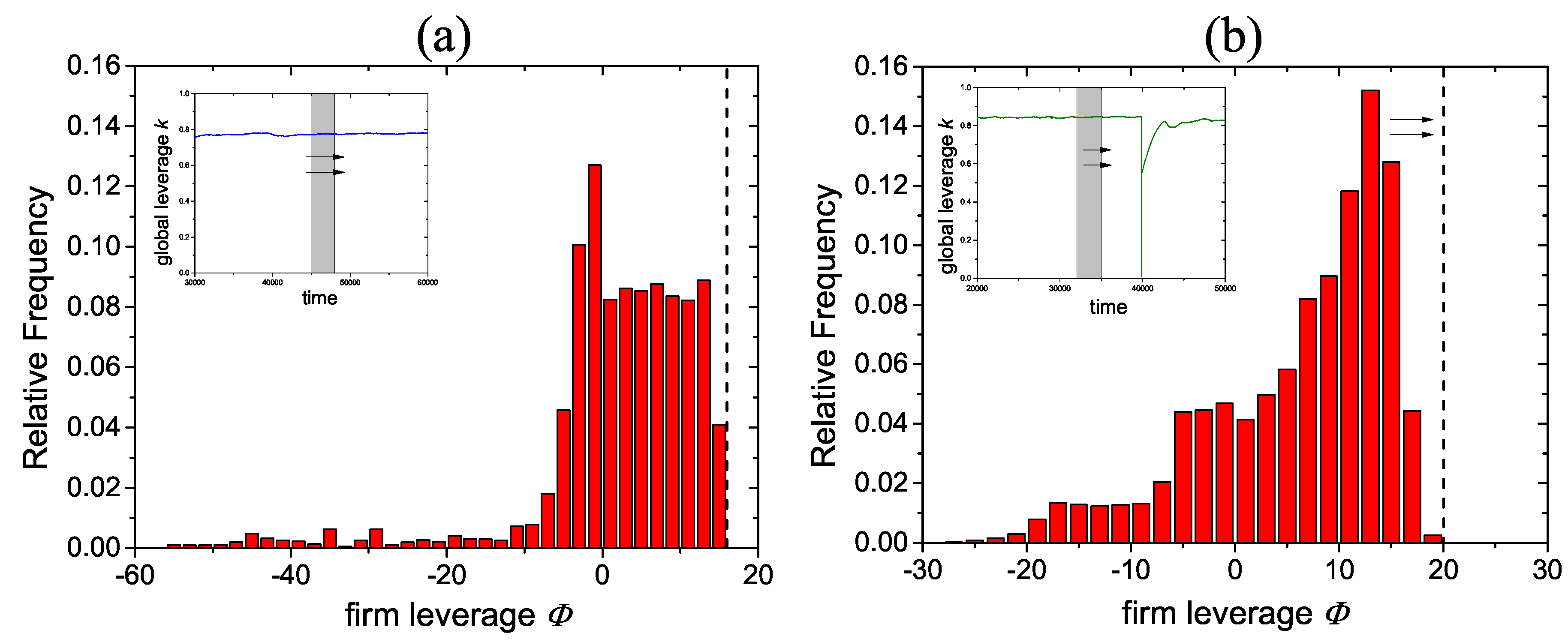
4.4. The Origins of Endogenous Crises

The variation of phase diagram motivates us to investigate the influence of the heterogeneity in firms’ economic performance on the occurrence of endogenous crisis at the micro-level. Remind that a firm agent’s fragility Φ i ( t ) , defined as the ratio of its cash balance ε i ( t ) to its scale of production Y i ( t ) w i ( t ) , would decide the firm’s fate (bankrupt or not). Firms with positive values of Φ i ( t ) are in debt and firms with negative values of Φ i ( t ) are holding cash and have no debt. When Φ i ( t ) hits the threshold, which is θ = 15 here, the corresponding firm i would go bankrupt and its bad debt would be assumed by other agents in the system, leading to a jump of Φ i ( t ) to zero. The bad debt of a bankrupt firm would cause a shock to the households’ wealth (thus cutting demand in the next round), and to the financial fragilities of the firms with net cash. Figure 5 give the distributions of the individual firms’ leverage Φ for 3000 time steps in EC and FE phase of Mark0. In FE phase of Mark0, as long as sufficient liquidity is provided, e.g., θ = 15 here, all the underlying Φ i ( t ) would safely fluctuate below the boundary θ , hence no firm would go bankrupt and the unemployment rates is stable and near zero. The distribution of Φ is nearly symmetric and gaussian-like (Figure 5a). As the provided liquidity is decreased to θ = 5 , a cluster of indebted firms appears (Figure 5b), which can be identified by the distribution peak in the positive axis of Φ . While the distribution of Φ in FE phase is stationary, the distribution peak in EC would move towards the threshold θ (the vertical dashed line) as the shade area in the subfigure (indicating the time window of the data samples) get closer to the collapse point of the global leverage k. In fact, the endogenous crises occur when the peak bumps into the thresholds θ .
Figure 6 gives the distributions of the individual firms’ leverage Φ for 3000 time steps in FE and EC+ phase of HoP-Mark0. Although the unemployment rates in FE phases (the blue lines in Figure 2b and Figure 4b) of Mark0 and of HoP-Mark0 are similar, from the perspective of Φ distribution (Figure 5a and Figure 6a), one can notice that the low and stable unemployment have different underlying dynamics in the two models. In FE phase of HoP-Mark0, the bankruptcies of the firms with poor economic performance are quite frequent. Because the impact of the bankruptcies is not strong so that it can be absorbed by the firms with good financial conditions, no macroscopic crisis would be observed. The shape of the distributions of firms’ Φ would not change in FE phase of HoP-Mark0 as well. As the liquidity is increased to θ = 20 , the higher liquidity would not cause any change in Mark0 and the Φ distribution would be the same as the one when θ = 15 . However, in HoP-Mark0, the cluster of the indebted firms would appear again due to the prolonged survival time of the disadvantageous firms. The existence of the few advantageous firms becomes sort of “liquidity black hole”—the liquidity would not be used to prevent the endogenous crises but be absorbed by the advantageous firms. Moreover, the indebted firms would be allowed to accumulate higher leverages, due to the excessive liquidity so that an enhanced endogenous crisis would occur when the cluster bumps into the threshold. The time evolutions of the firms’ leverage Φ are shown in the Appendix A to help readers understand the underlying dynamics.
Interestingly, it is notable that the global leverage k is quite stable before the occurrence of the collapse in this situation and thus it can no longer be used as a measure of crisis risk in this phase. In Section 6, we would propose an adjusted global leverage which can be used as a risk indicator when heterogeneity of firms’ economic performance is considered and excessive liquidity is injected.

5. Other Factors and the Robustness of Crises

In reality, there can be factors that would reduce the heterogeneity of firms’ economic performance. For instance, firms with good economic performance may pay higher wages and bonuses, thus reducing the net profits; besides, even if a firm has high profit margin, production cycle may lead to mismatch between supply and demand and cause losses. In this section, production cycles and variable wages would be incorporated in the model to examine robustness of the phase diagram, particularly for EC and EC+ phase.

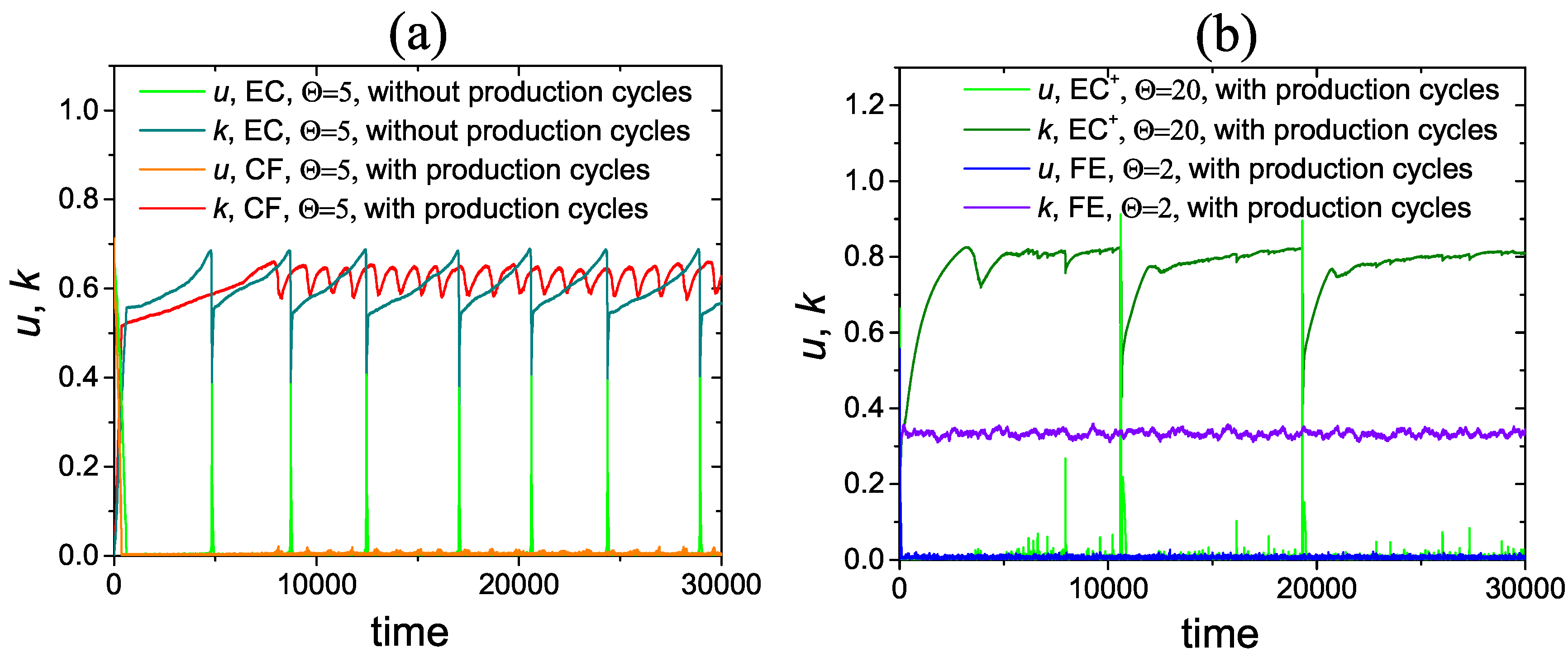
5.1. Production Cycles

In Mark0, the firms can make plans to increase or decrease their production, then fulfil the production and launch the products to the market immediately after they detect the imbalance between demand and supply in the market. However, in reality, the rebalance could be time consuming process, which usually cause a time lag. Note that this time lag was believed to be the mechanism accounting for the inventory cycles, also known as the Kitchin cycle [52]. The time lag itself may be induced by different kinds of factors: (1) the time-costing manufactory process, e.g., the manufactory of an airplane can take years; (2) the complex decision-making process for the managers, e.g., managers from different departments need to have meetings to reach an agreement; (3) the natural limitation of growth cycle, e.g., the production adjustment for agricultural commodities cannot be implemented until the next planting season. Regardless of different origins, we may use the term “production cycles” to represent the synthetic effects of the time lag discussed above.
Because of the existence of time lag between the production and sale process, the current production of firm i can only become the supply S i , which can be actually available to the households, to the market after τ i time steps:
Y i ( t ) = S i ( t + τ i ) .
Clearly, a smaller τ i indicates a shorter product cycle so that firm i can react to the market imbalance more promptly. When the time lag vanishes, τ i = 0 , the firm launches its products to the market without delay, just the same as the firms do in Mark0. The adjustment rules for price and production, the households’ behaviour and the bankruptcy and revival rules are the same as in Mark0. The firm’s accounting will be changed to:
ρ i ( t ) = p i ( t ) min [ S i ( t ) , D i ( t ) ] Y i ( t ) .
Thus, besides the challenge of predicting the market demand in a longer time horizon, the production cycles also cause cash flow problems because the current realized revenue p i ( t ) min [ S i ( t ) , D i ( t ) ] may not match the current production cost Y i ( t ) which can only be turned into revenue after τ i time steps. The other change is that the average price will be calculated according to the price of the products on the market but not the products still in production, p ¯ ( t ) = i p i ( t ) S i ( t ) i S i ( t ) . Lastly, we assume that the product price can be adjusted without time delay, though firms in real situations may have some sluggishness in price adjustments.
The effect of the production cycles is quite counter-intuitive. In traditional economic theory, the existence of production cycles reduces operational efficiency of firms and is deemed to have negative effect on the market efficiency. However, in Mark0, production cycles can bring positive effects on the macroscopic performance of the system. Under the same parameter setting, while the FE, RU and FU phases are kept unchanged and the phase boundaries are similar to the phase diagram of Mark0, however, EC phase would be replaced by a new phase, cyclical fluctuation (CF) phase. In contrast with the large spikes caused by synchronized collective behaviors of firms in the EC phase, we can observe in the CF phase only small quasi-periodical fluctuations in the unemployment rates (Figure 7a). In HoP-Mark0, the production cycles also have a stabilizing effect: the original EC phase is replaced by the FE phase. In fact, according to the discussion about the heterogeneous economic performance of firms and the endogenous crisis, it can be expected that the production cycles would mitigate the robust endogenous crisis - converting EC phase to CF phase in Mark0 and converting EC phase to FE phase in HoP-Mark0. The validity of the simple heuristic strategy for production implemented by the firm agents in the model is very dependent on the prompt adjustments based on the most recent market imbalance. Therefore, the introduction of production cycles would increase the prediction error of firm agents and thus largely weaken the heterogeneity of firms’ economic performance, i.e., a lucky firm can only maintain its economic advantage for very few time steps, meanwhile the indebted firms will go bankrupt quickly. The result of the very frequent bankruptcies is that total debt risk will not be accumulated.
However, we find that EC+ phase is robust against the introduction of the production cycles (Figure 7b). In HoP-Mark0, even if the production cycles would reduce the profitability of all the firms, the advantageous firms can still outperform the disadvantageous in the environment with excessive liquidity and eventually the large financial gap between the advantageous and the disadvantageous have to be relieve through the occurrence of crisis.

5.2. Variable Wages

A set of simple wage updating rules are as follows [10]:
If Y i ( t ) < D i ( t ) and ρ i ( t ) > 0 : w i ( t + 1 ) = w i ( t ) 1 + γ w 1 u ( t ) ξ i ( t ) If Y i ( t ) > D i ( t ) and ρ i ( t ) < 0 : w i ( t + 1 ) = w i ( t ) 1 γ w u ( t ) ξ i ( t ) In the other cases : w i ( t + 1 ) = w i ( t ) .
where γ w is a parameter controlling the magnitude of wage adjusting and ξ i ( t ) an independent random variable from a uniform distribution U(0,1). When a firm raises its wage, w i ( t + 1 ) would also be capped by the “break-even” point ρ i ( t ) = 0 , thus, w i ( t + 1 ) = min w i ( t + 1 ) , p i ( t ) min [ Y i ( t ) , D i ( t ) ] Y i ( t ) . The logic behind the rule is quite simple: when a firm makes profit and its products is in short supply, the firm will raise wages based on how tight the labour market is (i.e., depends on the employment rate, 1 u ( t ) ); when a firm makes losses and its supply exceeds demand, the firm will reduce its wage to make an attempt to return to profit.
The main effects brought by the wage dynamics in Mark0 are the appearance of inflation and the shrinking of EC region [10]. In HoP-Mark0, we employed the same wage updating rules and found it has similar effects. If using the ratio γ w / γ p as a magnitude measure of the relative wage flexibility, highe γ w / γ p would have a stronger stabilizing effect. In the phase diagram, EC region would be smaller as γ w / γ p is increased. Furthermore, as long as γ w / γ p > 0.01 , EC+ phase would disappear (Figure 8a). The disappearance of EC+ phase can be expected: EC+ phase relates to the increasing wealth gap between the advantageous firms and the disadvantageous firms in the environment with excessive liquidity. The proposed wage updating rules will make the advantageous firms increase the wages until the wages are capped by the “break-even” point. Thus, the excessive profits of the advantageous firms would be quickly redistributed through wages and the wealth gap would be eliminated, as long as the relative wage flexibility is high enough.
Inflation and deflation can also be observed in HoP-Mark0 when the wage updating rules are incorporated (Figure 8b). In the “bad” economy (FU phase, R < R c ), deflation and high unemployment rate persist. When R R c , the liquidity parameter θ takes over the status of the modeled economy. For θ < θ RU EC , there is zero inflation in the price index p ¯ ( t ) and the unemployment rates stay high but remain stable; for θ RU EC < θ < θ EC FE , inflation and deflation will appear alternately; for θ > θ EC FE , inflation and full employment persist. As was mentioned above, when the firms adopt the wage updating rules but the relative wage flexibility is relatively low in an environment with excessive liquidity, EC+ phase would appear. Interestingly, in EC+ phase, the price index is characterized by long-term inflation but occasionally price collapses induced by the endogenous crises (Figure 9).

6. Implication on the Measurement of Risk for Endogenous Crises

In Mark0, the global leverage k can be used as a measure of risk in EC phase. In the no-crisis phases (FE and RU), k would stabilize at certain levels. But in EC phase, it keeps increasing until the occurrence of crisis, which would lead to a quick deleveraging process. However, when the firms present heterogeneity of economic performance (EC+ phase of HoP-Mark0), the global leverage k does not show clear increase before crises (Figure 3b and Figure 7b). Thus, one can hardly detect the increasing risk in the system through the global leverage. This is due to the fact that only the aggregate debt and equity are used in the calculation of the global leverage. As discussed in Section 3.3, the endogeneous crises, whether in EC phase or in EC+ phase, are related to the shapes and the time evolutions of the Φ distributions. In HoP-Mark0, when the liquidity is just enough, i.e., θ EC FE < θ < θ FE EC + , the excessive liquidity of the advantageous firms would be used to cover the bad debt of the disadvantageous firms. Thus, the advantageous firms would not increasingly occupy the liquidity and the risk is defused continually (Figure 6a). However, when there is excessive liquidity, i.e., θ > θ FE EC + , the advantageous firms would absorb the liquidity and grow larger and larger, meanwhile the disadvantageous firms would survive for a prolonged time and accumulate higher leverages (Figure 6b). Therefore, the global leverage k would underestimate the risk in HoP-Mark0 because it does not take the Φ distributions into account. To correctly measure the risk accumulation in the HoP-Mark0, i.e., to alleviate the risk-underestimating problem brought by the advantageous firms, we propose a new variable, the adjusted global leverage k x % adj
k x % adj ( t ) = ε ( t ) H ( t ) + ε + ( t ) ε x % ( t ) ,
where ε x % (t) is the summation of the cash occupied by the most advantageous x % firms in all the firm agents. Figure 10 gives the original global leverage k and the adjusted global leverage k 15 % adj ( t ) in the moderate liquidity case ( θ = 15 ) and the excessive liquidity case ( θ = 20 ), corresponding to FE and EC+ phase in HoP-Mark0. In FE phase ( θ = 10 ), the adjusted global leverages would fluctuate around an equilibrium level, suggesting that a stable distribution of liquidity is reached (Figure 10a). The adjusted global leverage k 15 % adj ( t ) clearly indicates the increasing leverage risk before the occurrence of crises in EC+ phase, while the global leverage k is stable before crisis (Figure 10b).

7. Conclusions

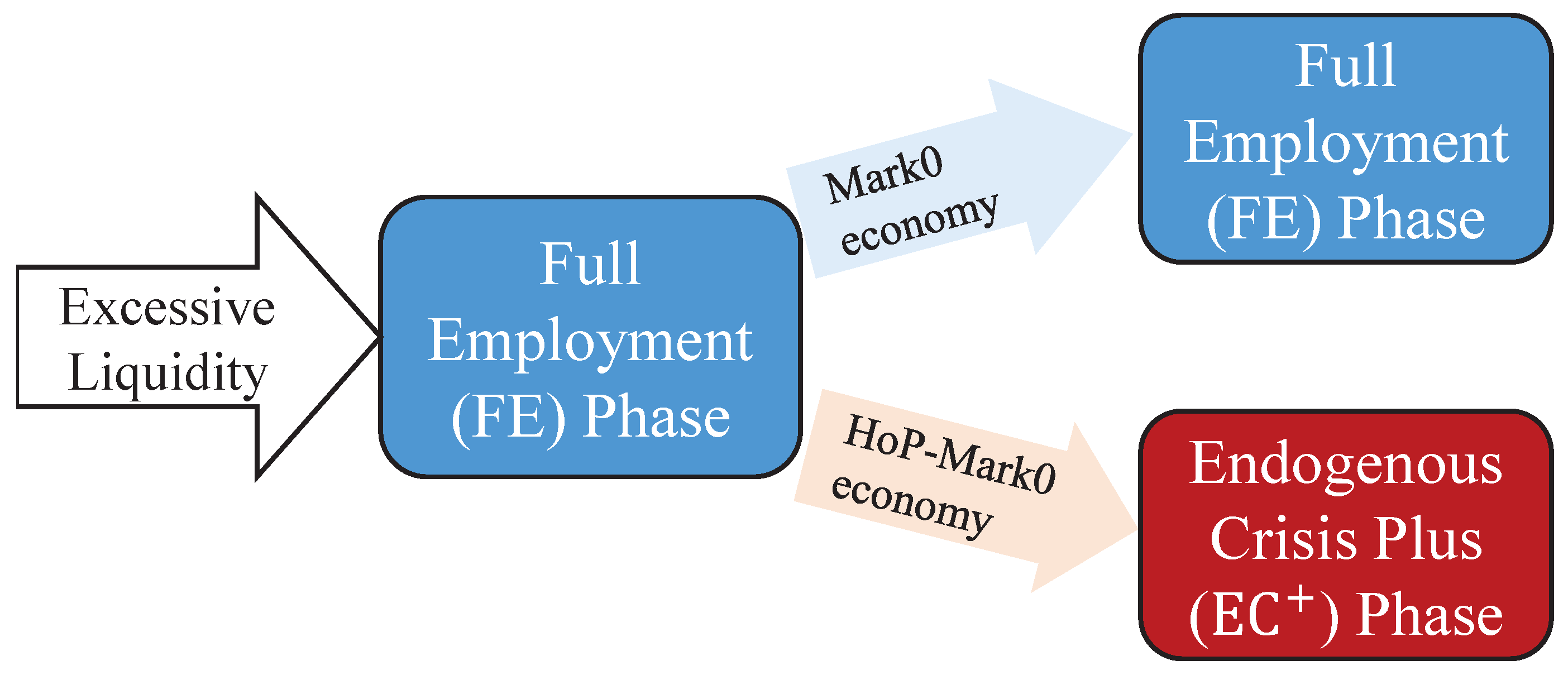
7.1. Summary of Results and Insights

In this research, we have extended a well-studied ABM for maroeconomy (Mark0) to a version integrated with heterogeneity of firms’ performance (HoP-Mark) to investigate the relations between firm heterogeneity and endogeneous crises in theory. Compared with the Mark0 results where high liquidity guarantees the stability of economy, we find in HoP-Mark0 that excessive liquidity could endanger the system and trigger rarer but more severe crises with enhanced rate of bankrupcty and unemployment by enlarging the gap between firm’s financial status is huge (Figure 11). Further model explorations verify that the such catastrophic crises would be mitigated to some extent under the influences from factors reducing the firm heterogeneity of profitability, typically the production cycles of firms and the variable wage system. The reason why firm heterogeneity changes the role of liquidity is revealed by time evolutions of the distribution of firms’ accumulating wealth. In Mark0, given sufficient liquidity, the homogeneous firm setting ensures a stable Gaussian-like distribution of firms’ wealth; yet in our model, an incessant polarization of wealth distribution into an highly skewed shape is tiggered by excessive liquidity, resulting in a situation where a large ratio of the total market value is contributed only by a small number of “winner” companies. Interestingly, we also find that the global leverage ratio proposed in Mark0 [10] cannot be used to measure the risk of catastrophic crises in HoP-Mark0. To fix this deficiency, we further propose an adjusted global leverage ratio which take the firm heterogeneity into account so as to effectively measure the risk in the model economy.
This finding may provide insights into some urgent issues. Nowadays, governments and central banks are accustomed to adopt expansionary monetary policies to spur the recovery of an economy when there were recessions or crises. Such expansionary monetary policies, which will flood the economy with liquidity, have been proven effective in raising the employment rates and avoiding deflations.For instance, the central banks have been providing excessive liquidity in reponse to the financial crises (QE1, QE2 and QE3 in the U.S., Abenomics in Japan and the 4 trillion yuan stimulus plan in China). Nevertheless, the ultra-loose monetary policies have been proven effective in raising the employment rates and avoiding deflations after the crises in a short term, these policies also arouse concerns about their side-effects, such as unexpected inflation [53] and increased income and wealth inequality [54]. Based on our results(HoP-Mark0), we can interpret a possible side-effect of excessive liquidity from the perspective of firm’s heterogeneity as follows:
In different stages of the economic development, there were always some firms outperforming others and they may become giant companies in the long term. These giants constantly win money from those small firms in the competition for household’s demand and absorbe the liquidity of the whole system. As a result, an increasing portion of firms struggle on the verge of brankruptcy with extremely high debts and leverages so that there is a high probability for these firms to get bankrupted synchronously, which then endanger the healthy firms. Ironically, the abnormal distrubution of firm financial status is induced by excessive liquidity although the trend of increasing gap between firms is inevitible. By contrast, an appropriately high liquidity which allows more endangered firms to die at different moments can avoid the synchronization of their bankruptcies, and overall maintain a stable economy.
Moreover, traditional leverage ratio based on aggregate values of individuals may underestimate the systemic risk. To correctly measure the risk, the leverage ratio should be adjusted to filter the influence brought by those “liquidity-absorbing entities”. In a real economy, it will be not easy to identify the “abnormal” divergence in the economic performance of firms. Some indicators, such as Lerner Index (LI) [55] and Herfindahl-Hirschman index (HHI) [56], which are commonly used to evaluate the degree of market concentration, may be relevant ones. Nevertheless, the calculations of these indicators do not reflect the firms’ cash flows. When excessive liquidity is provided, the divergence of firms’ abilities in earning cash flows is the key reason for the emergence of enhanced endogeneous crises in the modeled economy.
The methodology and theory also apply to economic systems on different scales. For instance, one can similarly reason the influence of a loose monetary environment in the world with large-scale trade imbalances among countries, or the consequence of heavy subsidies (corresponding to the excessive liquidity) in a sector with the profitabiliy of firms largely dispersed. We thus can propose some suggestions for the sustainability of economic prosperity from two prospectives. Firstly in a broad sense, risk measures considering distributional rather than additional values of firms, industries and even countries should be developed to alarm severe economic crises (especially global ones) because a well-functioned economy is always a precondition for the pursuit of sustainability. Secondly in a narrow sense, to avoid economic shocks brought by some industrial policies, governments should support some specific sectors with prudence. An example at hand is that they provide substantial subsidies to the sectors related to renewable energies and green vehicles. There is an ongoing debate about whether or not to continue these subsidies. We suggest that money should be carefully injected in case of any excessive liquidity that may ruin rather than support the sectors.

7.2. Limitations and Future Tasks

Finally, we shall discuss the limitations of this work at this stage and point out some future directions of improvement. The limitations are twofold.First, for the purpose of feasibility, many other fundamental elements have not been considered in the model, such as the interest rate, the capital investment of firms, the import and export of products. All the conclusions shown here are established under many simplifications for a closed system and just serve as benchmarks for sophisticated extensions to be compared with. Second, the minimal ABM models suffice more to give the qualitative explanations but lack of quantitative validity because the parameters in the models are difficult to be calibrated with real data. This feature of our models also undermines its applicability in practical uses for regulators. In fact, we have investigated some emperical data and find that the distribution of firm’s assets could tend to be highly skewed (implying a soaring inequality among firm’s wealth) before crises occur [57,58,59], as shown in HoP-Mark0. But more effort should be made on the validation of our hypothesis about the role of excessive liquidity in exacerbating inequality and in triggering the severe endogenous crises. One possible way to link real data and our model is to directly construct the distribution of financial fragility (using some surrogate variables from the financial statement of firms, for instance, the quick ratio = liquidity assets/current liabilities) before and after an economic crisis, which could be a very time-consuming project.
Accordingly, future tasks encompass several directions (1) integrating more ingredients of interest into the model, especially those regarding the heterogeneous behaviors of firms or households and those for an open system to theoretically explore the factors that might be critical to reduce the risk of crises; (2) doing paralelled statistical analyses of financial fragiligy of firms in both the model and emperical data to qualitatively validate our hypothesis regarding the role of excessive liquidity; (3) relating this ABM to some models in the DSGE style and trying to quantitatively reproduce the historical data for a better practical use.

Author Contributions

Conceptualization, W.Z. and Y.C.; Formal analysis, W.Z. and Y.L.; Methodology, W.Z. and Y.L.; Software, W.Z.; Supervision, Y.C.; Writing—original draft, W.Z. and Y.L.; Writing—review and editing, Y.L. and Y.C.

Funding

This research received no external funding.

Acknowledgments

We appreciate the valuable advises of the two anonymous reviewers and the editors who help improve the quality of this work. We are especially grateful to Dongying Ju for a careful reading of the manuscript and for his important input and suggestions.

Conflicts of Interest

The authors declare no conflict of interest.

Abbreviations

The following abbreviations are used in this manuscript:
ABMAgent-based model
DSGEDynamic stochastic general equilibrium
REResidual employment
ECEndogenous crisis
FEFull employment
FUFull unemployment
CFCyclical fluctuation
HoPHeterogeneity of economic perfomance

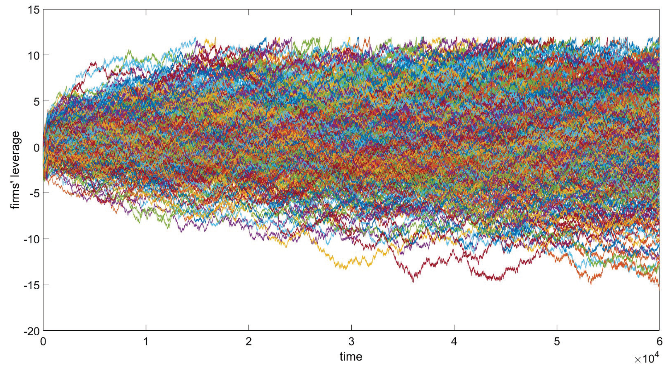
Appendix A. Evolution of Firms’ Wealth in Mark0 and HoP-Mark0

Figure A1, Figure A2, Figure A3 and Figure A4 give the time evolutions of the firms’ leverage in EC and FE phase in Mark0, and in FE and EC+ phase in HoP-Mark0, respectively. The firms with positive values of Φ are in debt while the firms with negative values of Φ are holding cash and have no debt. The values of Φ can be regarded as measures of wealth for the firms—the smaller Φ i ( t ) is, the more wealth is occupied by firm i. When Φ i ( t ) hits the default threshold, the corresponding firm i would go bankrupt and its bad debt would be assumed by other agents in the system, leading to a jump of Φ i ( t ) to zero. The collective bankruptcies of the firms indicate the occurrence of the endogenous crises in EC or the enhanced endogenous crises in EC+. The parameters other than θ are fixed as: N f = 500 , c = 0.5 , γ p = 0.05 , δ = 0.02 , β = 1 , ψ = 0.1 .
Figure A1. The time evolutions of the firms’ leverage in EC phase of Mark0 with θ = 5 . Each line represents one of the 500 firm agents.
Sustainability 11 03075 g0a1
Figure A2. The time evolutions of the firms’ leverage in EC phase of Mark0 with θ = 12 . Each line represents one of the 500 firm agents.
Sustainability 11 03075 g0a2
Figure A3. The time evolutions of the firms’ leverage in FE phase of HoP-Mark0 with θ = 12 . Each line represents one of the 500 firm agents.
Sustainability 11 03075 g0a3
Figure A4. The time evolutions of the firms’ leverage in EC+ phase of HoP-Mark0 with θ = 25 . Each line represents one of the 500 firm agents.
Sustainability 11 03075 g0a4

References

  1. Spangenberg, J.H. Economic sustainability of the economy: concepts and indicators. Int. J. Sustain. Dev. 2005, 8, 47–64. [Google Scholar] [CrossRef]
  2. Anand, S.; Sen, A. Human development and economic sustainability. World Dev. 2000, 28, 2029–2049. [Google Scholar] [CrossRef]
  3. Schneider, F.; Kallis, G.; Martinez-Alier, J. Crisis or opportunity? Economic degrowth for social equity and ecological sustainability. Introduction to this special issue. J. Clean. Prod. 2010, 18, 511–518. [Google Scholar] [CrossRef]
  4. Geels, F.W. The impact of the financial–economic crisis on sustainability transitions: Financial investment, governance and public discourse. Environ. Innov. Soc. Transit. 2013, 6, 67–95. [Google Scholar] [CrossRef]
  5. Novo-Corti, I.; Țîrcă, D.M.; Ziolo, M.; Picatoste, X. Social Effects of Economic Crisis: Risk of Exclusion. An Overview of the European Context. Sustainability 2019, 11, 336. [Google Scholar] [CrossRef]
  6. Stockhammer, E. Rising inequality as a cause of the present crisis. Camb. J. Econ. 2015, 39, 935–958. [Google Scholar] [CrossRef]
  7. Atkinson, A.B.; Bourguignon, F. Handbook of Income Distribution; Elsevier: Amsterdam, The Netherlands, 2014; Volume 2. [Google Scholar]
  8. Galbraith, J.K. Inequality and Instability: A Study of the World Economy Just before the Great Crisis; Oxford University Press: Oxford, UK, 2012. [Google Scholar]
  9. Kumhof, M.; Rancière, R.; Winant, P. Inequality, leverage, and crises. Am. Econ. Rev. 2015, 105, 1217–1245. [Google Scholar] [CrossRef]
  10. Gualdi, S.; Tarzia, M.; Zamponi, F.; Bouchaud, J.P. Monetary policy and dark corners in a stylized agent-based model. J. Econ. Interact. Coord. 2017, 12, 507–537. [Google Scholar] [CrossRef]
  11. Stiglitz, J.E. Towards a General Theory of Deep Downturns; Technical Report; National Bureau of Economic Research: Cambridge, MA, USA, 2015. [Google Scholar]
  12. Colander, D.; Howitt, P.; Kirman, A.; Leijonhufvud, A.; Mehrling, P. Beyond DSGE models: Toward an empirically based macroeconomics. Am. Econ. Rev. 2008, 98, 236–240. [Google Scholar] [CrossRef]
  13. Bookstaber, R. The End of Theory: Financial Crises, the Failure of Economics, and the Sweep of Human Interaction; Princeton University Press: Princeton, NJ, USA, 2017. [Google Scholar]
  14. Ormerod, P. Information cascades and the distribution of economic recessions in capitalist economies. Phys. A Stat. Mech. Appl. 2004, 341, 556–568. [Google Scholar] [CrossRef] [Green Version]
  15. Ormerod, P. Risk, recessions and the resilience of the capitalist economies. Risk Manag. 2010, 12, 83–99. [Google Scholar] [CrossRef]
  16. Kirman, A.P. Whom or what does the representative individual represent? J. Econ. Perspect. 1992, 6, 117–136. [Google Scholar] [CrossRef]
  17. Galí, J. Monetary Policy, Inflation, and the Business Cycle: An Introduction to the New Keynesian Framework; Princeton University Press: Princeton, NJ, USA, 2008. [Google Scholar]
  18. Fagiolo, G.; Roventini, A. Macroeconomic policy in DSGE and agent-based models. Revue de l’OFCE 2012, 5, 67–116. [Google Scholar]
  19. Blanchard, O. Do DSGE models have a future? Revista de Economía Institucional 2016, 18, 39–46. [Google Scholar] [CrossRef]
  20. Christiano, L.J.; Motto, R.; Rostagno, M. Risk shocks. Am. Econ. Rev. 2014, 104, 27–65. [Google Scholar] [CrossRef]
  21. Korinek, A.; Simsek, A. Liquidity trap and excessive leverage. Am. Econ. Rev. 2016, 106, 699–738. [Google Scholar] [CrossRef]
  22. Bilbiie, F.O. The New Keynesian Cross; University of Oxford: Oxford, UK, 2017. [Google Scholar]
  23. Delli Gatti, D.; Palestrini, A.; Gaffeo, E.; Giulioni, G.; Gallegati, M. Emergent Macroeconomics: An Agent-Based Approach to Business Fluctuations; Springer: Berlin, Germany, 2008. [Google Scholar]
  24. Pogson, M.; Smallwood, R.; Qwarnstrom, E.; Holcombe, M. Formal agent-based modelling of intracellular chemical interactions. Biosystems 2006, 85, 37–45. [Google Scholar] [CrossRef]
  25. Batty, M. Cities and Complexity: Understanding Cities with Cellular Automata, Agent-Based Models, and Fractals; The MIT Press: Cambridge, MA, USA, 2007. [Google Scholar]
  26. Bonabeau, E. Agent-based modeling: Methods and techniques for simulating human systems. Proc. Natl. Acad. Sci. USA 2002, 99, 7280–7287. [Google Scholar] [CrossRef] [Green Version]
  27. Sornette, D. Physics and financial economics (1776–2014): Puzzles, Ising and agent-based models. Rep. Prog. Phys. 2014, 77, 062001. [Google Scholar] [CrossRef]
  28. Janssen, M.; Ostrom, E. Empirically based, agent-based models. Ecol. Soc. 2006, 11, 37. [Google Scholar] [CrossRef]
  29. Wu, X.; Xu, Y.; Lou, Y.; Chen, Y. Low carbon transition in a distributed energy system regulated by localized energy markets. Energy Policy 2018, 122, 474–485. [Google Scholar] [CrossRef]
  30. Aoki, M.; Yoshikawa, H. Reconstructing Macroeconomics: A Perspective from Statistical Physics and Combinatorial Stochastic Processes; Cambridge University Press: Cambridge, MA, USA, 2011. [Google Scholar]
  31. Caiani, A.; Godin, A.; Caverzasi, E.; Gallegati, M.; Kinsella, S.; Stiglitz, J.E. Agent based-stock flow consistent macroeconomics: Towards a benchmark model. J. Econ. Dyn. Control 2016, 69, 375–408. [Google Scholar] [CrossRef] [Green Version]
  32. Dawid, H.; Gemkow, S.; Harting, P.; Van der Hoog, S.; Neugart, M. The eurace@ unibi model: An agent-based macroeconomic model for economic policy analysis. Bielef. Work. Pap. Econ. Manag. 2012. [Google Scholar] [CrossRef]
  33. Deissenberg, C.; Van Der Hoog, S.; Dawid, H. EURACE: A massively parallel agent-based model of the European economy. Appl. Math. Comput. 2008, 204, 541–552. [Google Scholar] [CrossRef] [Green Version]
  34. Gatti, D.D.; Desiderio, S.; Gaffeo, E.; Cirillo, P.; Gallegati, M. Macroeconomics from the Bottom-Up; Springer Science & Business Media: Berlin, Germany, 2011; Volume 1. [Google Scholar]
  35. Dosi, G.; Fagiolo, G.; Roventini, A. Schumpeter meeting Keynes: A policy-friendly model of endogenous growth and business cycles. J. Econ. Dyn. Control 2010, 34, 1748–1767. [Google Scholar] [CrossRef] [Green Version]
  36. Bouchaud, J.P.; Gualdi, S.; Tarzia, M.; Zamponi, F. Optimal inflation target: Insights from an agent-based model. Econ. Discuss. Pap. 2017. [Google Scholar] [CrossRef]
  37. Gualdi, S.; Tarzia, M.; Zamponi, F.; Bouchaud, J.P. Tipping points in macroeconomic agent-based models. J. Econ. Dyn. Control 2015, 50, 29–61. [Google Scholar] [CrossRef] [Green Version]
  38. Tesfatsion, L. Agent-based computational economics: Growing economies from the bottom up. Artif. Life 2002, 8, 55–82. [Google Scholar] [CrossRef]
  39. McCoy, B.M.; Wu, T.T. The Two-Dimensional Ising Model; Courier Corporation: Chelmsford, MA, USA, 2014. [Google Scholar]
  40. Yang, C.N. The spontaneous magnetization of a two-dimensional Ising model. Phys. Rev. 1952, 85, 808. [Google Scholar] [CrossRef]
  41. Goldenfeld, N. Lectures on Phase Transitions and the Renormalization Group; CRC Press: Boca Raton, FL, USA, 2018. [Google Scholar]
  42. Bak, P. How Nature Works: The Science of Self-Organized Criticality; Springer Science & Business Media: Berlin, Germany, 2013. [Google Scholar]
  43. Challet, D.; Marsili, M.; Zhang, Y.C. Minority games: Interacting agents in financial markets. In OUP Catalogue; Oxford University Press: Oxford, UK, 2013. [Google Scholar]
  44. Challet, D.; Zhang, Y.C. Emergence of cooperation and organization in an evolutionary game. Phys. A Stat. Mech. Appl. 1997, 246, 407–418. [Google Scholar] [CrossRef] [Green Version]
  45. Cont, R.; Bouchaud, J.P. Herd behavior and aggregate fluctuations in financial markets. Macroecon. Dyn. 2000, 4, 170–196. [Google Scholar] [CrossRef]
  46. Alfi, V.; Cristelli, M.; Pietronero, L.; Zaccaria, A. Minimal agent based model for financial markets I. Eur. Phys. J. B 2009, 67, 385–397. [Google Scholar] [CrossRef] [Green Version]
  47. Alfi, V.; Cristelli, M.; Pietronero, L.; Zaccaria, A. Minimal agent based model for financial markets II. Eur. Phys. J. B 2009, 67, 399–417. [Google Scholar] [CrossRef] [Green Version]
  48. Mantegna, R.N.; Stanley, H.E. Introduction to Econophysics: Correlations and Complexity in Finance; Cambridge University Press: Cambridge, UK, 1999. [Google Scholar]
  49. Gualdi, S.; Bouchaud, J.P.; Cencetti, G.; Tarzia, M.; Zamponi, F. Endogenous crisis waves: Stochastic model with synchronized collective behavior. Phys. Rev. Lett. 2015, 114, 088701. [Google Scholar] [CrossRef]
  50. Anderson, S.P.; De Palma, A.; Thisse, J.F. Discrete Choice Theory of Product Differentiation; MIT Press: Cambridge, MA, USA, 1992. [Google Scholar]
  51. Porter, M.E. How competitive forces shape strategy. In Readings in Strategic Management; Springer: Berlin, Germany, 1989; pp. 133–143. [Google Scholar]
  52. Kitchin, J. Cycles and trends in economic factors. Rev. Econ. Stat. 1923, 5, 10–16. [Google Scholar] [CrossRef]
  53. Thornton, D. The downside of quantitative easing. Econ. Synop. 2010. [Google Scholar] [CrossRef]
  54. Bank of England. Quarterly Bulletin Retrieved on 13th September 2018; Bank of England: London, UK, 2018. [Google Scholar]
  55. Lerner, A. The concept of monopoly and the measurement of monopoly power. In Essential Readings in Economics; Springer: Berlin, Germany, 1995; pp. 55–76. [Google Scholar]
  56. Rhoades, S.A. The herfindahl-hirschman index. Fed. Res. Bull. 1993, 79, 188. [Google Scholar]
  57. Gaffeo, E.; Gallegati, M.; Palestrini, A. On the size distribution of firms: additional evidence from the G7 countries. Phys. A Stat. Mech. Appl. 2003, 324, 117–123. [Google Scholar] [CrossRef]
  58. Kang, S.H.; Jiang, Z.; Cheong, C.; Yoon, S.M. Changes of firm size distribution: The case of Korea. Phys. A Stat. Mech. Appl. 2011, 390, 319–327. [Google Scholar] [CrossRef]
  59. Gao, B.; Chan, W.K.V.; Li, H. On the increasing inequality in size distribution of China’s listed companies. China Econ. Rev. 2015, 36, 25–41. [Google Scholar] [CrossRef]
Figure 1. A schematic diagram of the flows of money in Mark0 model.
Sustainability 11 03075 g001
Figure 2. The four phases in Mark0, FU: full unemployment; RU: residual unemployment; EC: endogenous crises; FE: full employment. (a) The phase diagram of Mark0 in the θ R plane, with the parameters: N f = 500 , c = 0.5 , γ p = 0.05 , δ = 0.02 , β = 1 , ψ = 0.1 . (b) Typical time series of the unemployment rates u ( t ) in the four phases.
Sustainability 11 03075 g002
Figure 3. (a) Typical time series of the global leverage k ( t ) in the four phases in Mark0. (b) Typical time series of the global leverage k ( t ) in the five phases in HoP-Mark0.
Sustainability 11 03075 g003
Figure 4. The five phases in HoP-Mark0, FU: full unemployment; RU: residual unemployment; EC: endogenous crises; FE: full employment; EC+: endogenous crises plus. (a) The phase diagram of HoP-Mark0 in the θ R plane with the parameters: N f = 500 , c = 0.5 , γ p = 0.05 , δ = 0.02 , β = 1 , ψ = 0.1 . (b) Typical time series of the unemployment rates u ( t ) in the five phases. π i of the firms are random numbers from a uniform distribution U(1, 3/2). A larger upper limit of the distribution would increase the region of EC+.
Sustainability 11 03075 g004
Figure 5. The distributions of firms’ leverage Φ . in FE and EC phase in Mark0, with N f = 2000 , c = 0.5 , γ p = 0.05 , δ = 0.02 , β = 1 , ψ = 0.1 . (a) FE: the distribution is calculated from the data sample during a period of 3000 time steps, indicated by the shaded region in the subfigure. The dashed line indicates the default threshold θ = 15 ; (b) EC: the distribution is calculated from the data sample during a period of 3000 time steps before the occurrence of a crisis, indicated by the shaded region in the subfigure. The dashed line indicates the default threshold θ = 5 .
Sustainability 11 03075 g005
Figure 6. The distributions of firms’ leverage Φ in FE and EC+ phase in HoP-Mark0, with N f = 2000 , c = 0.5 , γ p = 0.05 , δ = 0.02 , β = 1 , ψ = 0.1 . (a) FE: the distribution is calculated from the data sample during a period of 3000 time steps, indicated by the shaded region in the subfigure. The dashed line indicates the default threshold θ = 15 ; (b) EC+: the distribution is calculated from the data sample during a period of 3000 time steps before the occurrence of a crisis, indicated by the shaded region in the subfigure. The dashed line indicates the default threshold θ = 20 .
Sustainability 11 03075 g006
Figure 7. (a) Typical time series of the unemployment rates u ( t ) and the global leverage k ( t ) in Mark0. With the extension of production cycles, EC phase would be converted to cyclical fluctuations (CF) phase. (b) Typical time series of the unemployment rates u ( t ) and the global leverage k ( t ) in HoP-Mark0. With the extension of production cycles, EC phase would be converted to FE phase but EC+ phase is robust against this extension. The parameters: N f = 500 , c = 0.5 , γ p = 0.05 , δ = 0.02 , β = 1 , ψ = 0.1 , τ i are random numbers from a uniform distribution U(1,10).
Sustainability 11 03075 g007
Figure 8. (a) Typical time series of the unemployment rates u ( t ) with the extension of variable wages in HoP-Mark0. When the wage flexibility γ w / γ p > 0.01 , EC+ phase would be converted to FE phase. The parameters: N f = 1000 , c = 0.5 , γ p = 0.05 , δ = 0.02 , β = 1 , ψ = 0.1 , γ w / γ p = 0.1 . (b) The corresponding inflation rates in HoP-Mark0. FU, RU, EC and FE phase are featured with deflation, zero inflation, alternations of deflation and inflation and inflation, respectively. The inflation rates are calculated from the 50-step moving average of the average price p ¯ ( t ) .
Sustainability 11 03075 g008
Figure 9. The unemployment rates u ( t ) and the average price in EC+ phase of HoP-Mark0 with the extension of variable wages. When the wage flexibility γ w / γ p < 0.01 , EC+ phase would exist. The parameters: N f = 1000 , c = 0.5 , γ p = 0.05 , δ = 0.02 , β = 1 , ψ = 0.1 , γ w / γ p = 0.01 , θ = 25 .
Sustainability 11 03075 g009
Figure 10. (a) The global leverage k ( t ) , the adjusted global leverage k 15 % adj ( t ) and the corresponding unemployment rates u ( t ) in FE phase in HoP-Mark0. (b) The global leverage k ( t ) , the adjusted global leverage k 15 % adj ( t ) and the corresponding unemployment rates u ( t ) in EC+ phase in HoP-Mark0.
Sustainability 11 03075 g010
Figure 11. Different fates of the modeled economies after injecting excessive liquidity in models with a homogeneous setting (Mark0) and heterogeneous setting (HoP-Mark0) of firms’ economic performance.
Sustainability 11 03075 g011

