Prediction of Land Use and Land Cover Changes for North Sumatra, Indonesia, Using an Artificial-Neural-Network-Based Cellular Automaton


1
Graduate School for International Development and Cooperation, Hiroshima University, 1-5-1 Kagamiyama, Higashi-Hiroshima 739-8529, Hiroshima, Japan
2
Environmental and Forestry Research and Development Agency of Aek Nauli, Sibaganding, Simalungun 21174, North Sumatra, Indonesia
*
Author to whom correspondence should be addressed.
Sustainability 2019, 11(11), 3024; https://doi.org/10.3390/su11113024
Submission received: 16 April 2019
/
Revised: 24 May 2019
/
Accepted: 24 May 2019
/
Published: 28 May 2019
(This article belongs to the Section Sustainable Urban and Rural Development)
Abstract
:Land use and land cover (LULC) form a baseline thematic map for monitoring, resource management, and planning activities and facilitate the development of strategies to balance conservation, conflicting uses, and development pressures. In this study, changes in LULC in North Sumatra, Indonesia, are simulated and predicted using an artificial-neural-network-based cellular automaton (ANN-CA) model. Five criteria (altitude, slope, aspect, distance from the road, and soil type) are used as exploratory data in the learning process of the ANN-CA model to determine their impacts on LULC changes between 1990 and 2000; among the criteria, altitude and distance from the road have strong impacts. Comparison between the predicted and the real LULC maps for 2010 illustrates high agreement, with a Kappa index of 0.83 and a percentage of correctness of 87.28%. Then, the ANN-CA model is applied to predict LULC changes in 2050 and 2070. The LULC predictions for 2050 and 2070 demonstrate high increases in plantation area of more than 4%. Meanwhile, forest and crop area are projected to decrease by approximately 1.2% and 1.6%, respectively, by 2050. By 2070, forest and crop areas will decrease by 1.2% and 1.7%, respectively, indicating human influences on LULC changes from forest and cropland to plantations. This study illustrates that the simulation of LULC changes using the ANN-CA model can produce reliable predictions for future LULC.
1. Introduction
Land use refers to the purpose that land serves, for example, recreation, wildlife habitat, or agriculture. Land cover refers to the surface cover on the ground, whether vegetation, urban infrastructure, water, bare soil or other. Although the meanings of the terms are distinct, land use and land cover (LULC) are often used interchangeably. Identifying, delineating and mapping land cover is important for global monitoring studies, resource management, and planning activities. Identification of land cover establishes the baseline from which monitoring activities (change detection) can be performed and provides the ground cover information for baseline thematic maps. Moreover, land use applications involve both baseline mapping and subsequent monitoring, since timely information is required to know what current quantity of land is involved in what type of use and to identify the land use changes from year to year. Therefore, knowledge of LULC will help with the development of strategies to balance conservation, conflicting uses, and development pressures. Additionally, issues can be identified from LULC studies, such as the removal or disturbance of productive land, urban encroachment, and the depletion of forests suitable for species distribution [1].
Simulation of LULC changes provides the baseline scenario for use when predicting future scenarios and patterns in future development. Simulation of LULC changes can indicate anthropogenic impact, identify land use problems, such as the degradation and deforestation, and be used in land use planning [2]. Land use changes have been important aspects for regional and urban planning for centuries. Most of the research predicts land use changes using the independent variable with the highest correlation to those changes. Verburg et al. [3] illustrated that the multiscale characteristics of land use systems require new techniques to quantify neighborhood effects. Furthermore, Verburg et al. [3] also explicitly dealt with temporal dynamics and achieved a higher level of integration among disciplinary approaches and between models studying urban and rural land use changes. Multivariate spatial models [4], Markov analysis [5], cellular automata (CA) [3,6,7,8,9], neural-network-based CA [2], empirical-statistical models [10,11], optimization models [12], and agent-based models [13,14] have all been used in the simulation of land use change. More details on each method can be found in [15].
The CA is a common method for simulating the LULC change spatial evolution by estimating the state of a pixel according to its initial state, surrounding neighborhood effects and transition rules. A CA model can generate rich patterns and effectively represent nonlinear spatially stochastic LULC change processes [16,17]. The applications of CA models have been growing in urban development studies, with strong capabilities for simulating the spatiotemporal complexity of urban systems [18,19,20,21,22,23], and in the simulation of deforestation under the influences of natural hazards or human activities [24,25]. However, most of these studies simulate the dynamics of one individual land use, while in many cases, various LULC change processes occur at the same time and affect each other [16,26]. In addition, these models do not account well for the role of climate change in long-term land use pattern changes.
LULC changes from human activities hinder predictive use. The changes are dynamic, depending on many factors, such as politics, regulation, and economic and social conditions. Regarding this condition, projection analysis needs to appear in the simulation to predict possible future scenarios. Among many methodologies described, agent-based modelling combines the cellular model (representing the landscape of interest) with an agent-based model (representing decision-making entities) [27]. Meanwhile, the other models use machine learning to process changes based on historical events and factors that provide the input for change. One of the models is an artificial-neural-network-based cellular automaton (ANN-CA), which was developed to simulate multiple land use changes and complex land use systems [2]. This approach can be used to determine LULC changes by considering the possible factors that may influence the changes. Therefore, ANN-CA is utilized in this study.
The study of land use change in the Asian region has been undertaken for many years. For instance, in China, a land use change model was developed using geographic information system (GIS) to monitor and predict change in the land [12,16,23,28]. Furthermore, LULC change is monitored and detected by remote sensing and GIS in Indonesia [29]. This LULC change model is based on multicriteria analysis in the GIS programme. The criteria are weighted, based on the researcher’s input, to determine their relative impacts on the model. The subjectivity of the researcher’s input for the weights is the limitation in the model. This limitation needs to be addressed by reducing the subjectivity and uncertainty of the researcher’s input.
The LULC is an essential factor influencing species distributions. This factor is one of the important environmental factors for addressing human activities that will affect the area suitable for biological populations in the present and future. North Sumatra, as one of the provinces in Indonesia with large forest area, requires that attention be paid to its LULC due to the threats of conversion and forestland degradation. Therefore, this research aims to define the transition of land use changes in North Sumatra between two different years (1990 and 2000) and to predict and demonstrate future land use changes in 2050 and 2070 using the ANN-CA approach for forest conservation, land use management and development, and species distribution management in the future.
2. Study Area and Data
2.1. North Sumatra
North Sumatra is located between 0°34′6.39″ S–4°18′16.59″ N in latitude and 97°3′32.7″–100°25′27.85″ E in longitude in the western part of Indonesia, where it borders the Indian Ocean on the west and Malaysia to the east. On the north, North Sumatra borders the Aceh region, and on the south, it borders the Riau and West Sumatra regions. North Sumatra covers 26 regencies and seven cities with a total area of approximately 71,068.68 km2 (Figure 1).
North Sumatra has experienced massive development over the last three decades where industrialization has changed the land use of most of the area, followed by agricultural expansion [30]. The forest area in North Sumatra is one of the largest in Indonesia, with more than 1,206,881 ha of preservation forest and 51,600 ha of conservation forest. However, there is forest degradation resulting from forest disturbance, especially from land conversion [31]. Several changes impact the forest as the habitat for many tree species displaced by other functions or land use. Moreover, the cover has also changed from trees to buildings or crops.
The human interest in land allocation influences the planning in North Sumatra to support the development of the area to be more productive, rather than maintaining it as forest [30]. For instance, most of the residents choose crop plantation for restoration of tree cover, rather than favouring hardwood trees, in the Lake Toba catchment area [32]. The LULC changes result from conflicting land interests. Crop plantation expands to increase profit, reducing forest area [33]. These conditions require the LULC perspective to emphasize the future impact of the changes, especially for loss of forest biodiversity.
Since the 17th century, North Sumatra has become a famous regency for forest products, such as Sumatra benzoin from the Styrax sumatrana trees. This product has become the income source of primary importance for communities around the forested areas in North Sumatra [34]. However, North Sumatra faces a problem with space allocation due to the increase in the population and industries, especially palm oil, rubber, and log-forest product plantations owned by private companies [35]. S. sumatrana was threatened by land conversion. This conversion influences the species sustainability in North Sumatra. The spatial LULC information is crucial to analyze the potential area for this species to grow. Therefore, the purpose of LULC change prediction in this study is to contribute to regional planning and management for the distribution of S. sumatrana in North Sumatra, and this is the rationale for choosing North Sumatra as the study region.
2.2. Data and Criteria
The data collected and used in this study include a digital elevation model (DEM), road map, soil types and three LULC maps for 1990, 2000, and 2010, as presented in Table 1. The Advanced Spaceborne Thermal Emission and Reflection Radiometer Global Digital Elevation Model (ASTER GDEM) v2 is one of the most widely used DEM datasets and is used in this study. The road map and LULC maps were obtained from the Ministry of Environment and Forestry of Indonesia, and the soil type map was obtained from the Food and Agriculture Organization (FAO).
From the dataset, five criteria, including altitude, slope and aspect from the DEM, distance from the road from the road map, and soil type, were selected for further analysis. Then, the criteria were classified into the input data and the explanatory data in the LULC simulation and prediction. The three LULC maps are the input data, and the other criteria, altitude, slope, aspect, distance from the road, and urban density, belong to the explanatory data (Table 1).
The three LULC maps were converted into raster data using ArcGIS. The resolution was 30 arc seconds, with 25 categories. Then, the number of categories was reduced into 12 classifications by regrouping several categories as shown in Table 2. The airport is considered separately, since it is assumed to be unchangeable in land use.
3. Methodology
3.1. Artificial-Neural-Network-Based Cellular Automaton Model
The simulations of LULC change and prediction were conducted using the ANN-CA model. ANN is used to determine the transition probability of LULC using multiple output neurons for simulating multiple LULC changes, within the structure of ANN-CA presented in Figure 2. CA is used to model the LULC changes by applying the transition probabilities from the ANN learning process. The overall analytic procedure is described in the following steps (Figure 3), and QGIS and its MOLUSE module were utilized for the ANN-CA modelling [24].
Step 1: The first step is to define the inputs to the neural network for the simulation. The simulation is cell-based (pixel-based), and each cell has a set of n attributes (spatial variables) as the inputs to the neural network. The spatial variables can be represented by
where xi is the i-th attribute, and T is transposition.
The initial (1990) and final (2000) LULC maps, as well as the five exploratory maps, are loaded as input data. Since we use five criteria from exploratory maps and 12 categories in LULC maps, 17 attributes (spatial variables) for each cell are used for modelling and simulating LULC changes. All datasets are processed to retrieve the attributes and have the same spatial extent and resolution (30 arc seconds) in raster format.
Step 2: Each correlation between spatial variables is evaluated in a two-way raster comparison by selecting the first raster from one variable and the second raster from another variable. Then, the LULC area and changes for each category are computed between the initial (1990) and final (2000) time periods. The transition matrix showing the proportions of pixels changing from one category to another is also obtained from the computation.
Step 3: In this step, the transition probability is modelled by ANN. The neural network structure consists of three layers, namely, the input, hidden, and output layers (Figure 2). Each spatial variable is associated with a neuron in the input layer after scaling within the range of [0, 1]. Therefore, the 17 neurons corresponding to the 17 attributes are used in the input layer.
In the hidden layer, the signal received by the j-th neuron, netj(k,t), from the input layer for the k-th cell at time t was computed by
where is the weight between the input and the hidden layers, and is the i-th scaled attribute associated with the i-th neuron in the input layer with respect to the k-th cell at time t. In terms of the number of neurons in the hidden layer, the use of 2n + 1 is recommended to guarantee the perfect fit of any continuous functions, and reduction of the number of neurons may lead to lower accuracy. However, based on Wang [25], 2n/3 hidden neurons can generate results of almost similar accuracy while requiring much less time to train. Therefore, we used 12 hidden neurons in this study.
The output layer includes 12 neurons corresponding to the 12 classifications in LULC maps (Table 2). The l-th neuron in the output layer generates a value that represents the transition probability from the initial type to the l-th (target) type of LULC. The transition probability is obtained by the following equation according to the output function of a neural network.
where is the probability of conversion from the existing to the l-th type of LULC for the k-th cell at time t, and is the weight between the hidden and the output layers. A higher value indicates that the transition probability from the initial type to the lth type is larger.
An iterative neural network based on the back-propagation learning algorithm is designed to simulate land uses in this study. At each iteration, each neuron in the output layer generates a transition probability from an existing type to another type of land use. In this simulation, LULC change is determined by comparing the values of transition probability such that LULC will convert from the existing type to the type with the highest value of transition probability. If the same type of LULC has the highest transition probability, the state of the corresponding cell remains unchanged.
Step 4: Once the transition probability is obtained, then modelling of LULC change is carried out by the CA simulation. The CA consists of regular spatial lattices of cells, each of which can have any one of a finite number of states, depending on the states of neighboring cells [27]. CA considers the composition of associations of cells around one cell [36]. CA simulation usually involves many iterations to decide whether a cell is changed or not. A predetermined threshold value should be used to control the rate of change so that land use conversions occur step-by-step. If the highest transition probability is lower than the threshold value, which is 0.9 in this study based on Li and Yeh [2], then the cell remains unchanged. The threshold value varies from 0 to 1, and the large value of 0.9 is used to keep the LULC changes stable in each iteration, thus obtaining fine patterns of simulation [2]. The CA in urban areas in this study only divides the classification into urban and non-urban areas for simplicity, because, if multiple land uses are presented, the transition rules of urban CA models become substantially more complicated, since the simulation involves the use of a much larger set of spatial variables and weights and more complex model structures.
Step 5: Validation of the LULC simulation using values of the Kappa coefficient to evaluate and compare the real (reference) and predicted (simulated) LULC maps for 2010 is described in Section 3.2.
Step 6: After the validation, the predictions of the future LULC maps in 2050 and 2070 are computed, assuming the continuation of the current trends and dynamics of the LULC changes. The same weight values are utilized for the neural network in the simulation of future LULC changes.
3.2. Validation
The validation is carried out by comparing the predicted and the real LULC maps for 2010. The true agreement from this validation is measured by the Kappa coefficient.
The Kappa coefficient is widely used in LULC assessments for accuracy [37] to measure the true agreement between the observed agreement and chance agreement [38]. The Kappa coefficient is calculated by
where po is the proportion of observed agreements, and pe is the proportion of agreements expected by chance.
where pij is the i-th and j-th cell of the contingency table, piT is the sum of all cells in i-th row, pTjis the sum of all cells in j-th column, and c is the count of the raster category. The contingency table is a matrix form that illustrates the frequency distribution of the variables and is used to show the interrelation between i-th and j-th cells in this study. The interaction of every cell is tabulated into a matrix and calculated. The result explains the agreement of every criterion of each cell. Finally, the contingency table is used to express the percent agreement as a Kappa coefficient.
To determine the exploratory map using the five criteria, a number of simulations to predict the LULC changes for 2010 were conducted by using each criterion, alone and in combinations of two to five, for the exploratory data in the LULC simulation. The result of explanatory map analysis from the seven simulations with different combinations of variables is presented in Table 3.
As displayed in Table 3, the overall correctness and Kappa coefficients are high and similar. Among these values, the exploratory data with altitude and distance from the road and their combination produced the highest Kappa score of 0.83 and the highest percent of correctness of 87.28%. The highest Kappa value indicates that the two criteria, altitude and distance from the road, have greater impacts on LULC changes than the other criteria. The two criteria are illustrated in Figure 4. Table 4 demonstrates the transition matrix of the 12 LULC categories between 1990 and 2000. Then, the result is employed to simulate the prediction of LULC for the years 2050 and 2070.
4. Results and Discussion
The percentage of area changes is presented by a transformation matrix that is used as the input for the neural network to obtain the transition probability for every input and to produce the LULC output layer. The LULC transition matrix is produced by comparing the area percentages of the LULC categories between the years 1990 and 2000, as shown in Table 4.
The ANN-CA model shows the prediction of LULC for the year 2010 by calculating the transition probability of every cell in the layer between two different LULC raster maps by considering altitude and distance from the road as the explanatory variables. The validation was implemented by comparing the factual LULC in the year of 2010 with the predicted LULC of the same year. The simulation shows a percentage of correctness of 87.28% and a Kappa value of 0.83 by using altitude and distance from road as the explanatory map. The percentage of correctness shows the percentage of the predicted area that is precisely the same as the real area in the same year. The Kappa value shows the degree of accuracy and reliability in a statistical classification. The value of 0.83 shows high agreement between the two different LULC maps from the same year [39].
The difference between the predicted and the real LULC maps of 2010 is described in Table 5. A positive value in the second column shows the overestimation of the prediction over the real condition, while a negative value indicates the opposite. A value of zero occurs when the real and predicted maps are equal or have the same value. The third and fourth columns explain the changes of every classification from the initial year of 2000 to the predicted and the real maps in 2010, respectively. Furthermore, the deviation between the predicted and the real maps of the LULC classifications are displayed in Figure 5.
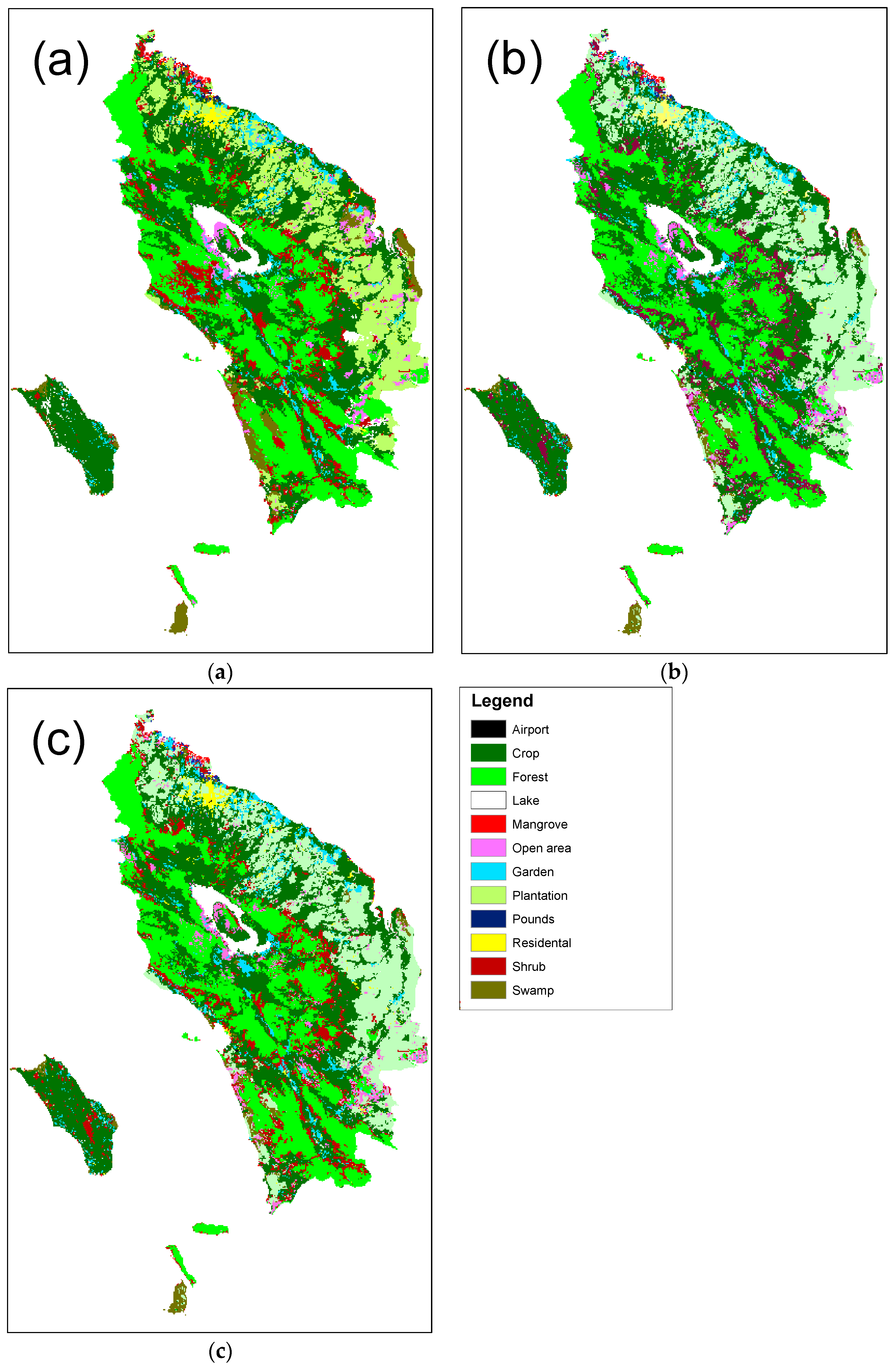
LULC prediction maps show the projected land use changes in 2050 and 2070 (Figure 6). The classifications in 2050 and 2070 are based on the classifications in 2000. To predict a species’ distribution, the land use change represents the percentage change in suitable land cover classification required for the species to survive in the future prediction. The percentages of these changes are presented in Table 6.
The percentages of shrub and garden fields are projected to increase by approximately 0.1547% and 0.3532% from 2000 to 2050 and 0.1768% and 0.3606% from 2000 to 2070, respectively. However, the crop and forest areas are projected to decrease by 1.24848% and 1.6779% from 2000 to 2050, followed by 1.2860% and 1.7256% from 2000 to 2070, respectively. Moreover, most of the classification will change to plantation. In 2050, the percentage of changes to plantation area are projected to increase to 4.1379% by 2050 and 4.1709% by 2070, respectively.
Land use change between 1990 and 2000 in the transition matrix shows that most of the area changed from forest and shrubland into plantations. Two areas with significant changes are forest by 0.045% and shrubland by 0.053% into plantation. However, the highest change was shrubland to crop area at 0.11%. This transition shows that human activities in forest and shrubland are high. The demands of land for human activities change LULC classifications from less profitable (the non-valuable classification: forest and shrubland, which are allotted lower economic profits) to a more profitable classification (valuable classification: plantation such as palm oil and rubber, which provide annual or seasonal income). This condition threatens the species in forest and shrubland by reducing the suitable area for species to survive. Other studies have demonstrated that changes in forest and crop area into oil palm plantation is higher in Indonesia, in particular on Sumatra Island [40,41].
The differences between the land use map from 2000 and those of 2050 and 2070 illustrate the high increases in plantation area of more than 4%, while the other classifications show changes of approximately 0%–1.8%. An increase in one classification indicates a decrease in other classifications. Higher changes of the categories into plantation indicate that the probability for plantation is higher than for the other categories. The changes were acquired by the ANN to weight the categories proportionally for use in the model.
5. Conclusions
The LULC is of critical importance and forms a baseline thematic map for monitoring, resource management, and planning activities. Moreover, the LULC can be used to develop strategies to balance conservation, conflicting uses, and development pressures. In this study, changes in LULC in North Sumatra, Indonesia, are simulated and predicted using the ANN-CA model.
Five criteria, including altitude, slope, aspect, distance from road, and soil type, are derived from a DEM, road map and soil type map, and utilized as exploratory data for training the ANN-CA model. In the simulation of LULC changes between 1990 and 2000, two criteria, altitude and distance from road, show high impacts on LULC changes. The Kappa index also indicates high agreement between the predicted and real LULC maps of 2010. Then, the ANN-CA model is used to predict the LULC changes for the years 2050 and 2070.
The LULC predictions for 2050 and 2070 show high increases in plantation area, which increase by more than 4% from the same category in 2010. Meanwhile, forest and crop areas are projected to decrease by approximately 1.2% and 1.6%, respectively, by 2050, and by approximately 1.2% and 1.7%, respectively, by 2070, relative to the 2010 LULC, indicating the human influences on LULC changing forest and cropland to plantations.
As described, among all regions in Indonesia, North Sumatra is one of the regions with great forest area that has been threatened by climate change and land use change [31]. In fact, North Sumatra has experienced massive development over the last three decades, as industrialization has changed the land use of most areas, followed by the agricultural expansion [30]. Therefore, there is forest degradation as the result of forest disturbance, especially from land conversion [31]. The human interest in land allocation lures the planning in North Sumatra to support the development of the region. Development changes the land to more productive uses, such as agriculture or industrial types, rather than preserving it as forest [30]. For instance, most of the residents choose crop plantations for reforestation rather than hardwood trees in the Lake Toba catchment area [42]. The resident corporations expand their plantations to increase profit and reduce the forest area [33]. This condition demands the LULC perspective to emphasize the future impact of the changes, especially on loss of forest biodiversity.
The ANN-CA model in this study is based on historical information and observes changes supported by explanatory variables. The CA demonstrates that the change of one pixel into another category relies on its neighborhood. The changes will continue until every pixel undergoes the changing process. The ANN-CA model might be more reliable in terms of reduced subjectivity and uncertainty when compared to other methods such as analytic hierarchy process (AHP) and technique for order preference by similarity to ideal solution (TOPSIS) for weighting criteria [43,44]. Moreover, this study illustrates that the ANN-CA model is successfully applied to conduct multiple LULC change simulations within one CA model by considering the complicated interactions and competition among different land use categories.
On the other hand, long-term effects altering the landscape dynamics, as exhibited in [26,45,46], due to climate factors, such as global warming, extreme weather events, etc., and ecological degradation, such as hydrological variation, soil erosion, etc., are not considered in this study. Moreover, this ANN-CA model does not consider planning and development factors in such a way as to determine demands for different land use types from the macro-scale perspective and to examine scenarios representing future development pathways [47,48]. Therefore, it should be noted that predicted future LULC changes obtained in this study are very limited in a conservative manner.
The forest area in North Sumatra, as described, is one of the largest in Indonesia with large preservation forest and conservation forest areas. However, there is forest degradation resulting from forest disturbance, especially from land conversion. The development of the region by human interests changes the land to more productive uses, such as agriculture or industrial types, rather than preserving it as forest. In general, the LULC changes occur as the impact of conflicts over land interests. For instance, the local residents choose crop plantations for reforestation, and corporations expand their plantations to increase profit and thus reduce forested area in the region. This condition demands the LULC perspective to emphasize the future impact of the change, particularly for loss of forest biodiversity. Therefore, the LULC changes predicted by this study can be used in sustainable forest management and regional planning.
In this study, however, other variables, such as climate, policy, regulation or human development, affecting LULC changes are not taken into account. Therefore, future investigation will be improved by including those variables.
Author Contributions
Conceptualization, methodology, analysis, validation, investigation, resources, writing, visualization, M.H.S. and H.S.L.; supervision, H.S.L.
Funding
This research is partly supported by the Grant-in-Aid for Scientific Research (17K06577) from JSPS, Japan.
Acknowledgments
The first author would like to thank the Ministry of Environment and Forestry and Planning Agency, Indonesia, for their support in this research and thanks all CHESS lab members at Hiroshima University for useful discussion and comments.
Conflicts of Interest
The authors declare no conflict of interest.
References
- Anderson, J.R.; Hardy, E.E.; Roach, J.T.; Witmer, R.E. A Land Use and Land Cover Classification System for Use with Remote Sensor Data; United States Department of the Interior: Washington, DC, USA, 1983; p. 28. [Google Scholar]
- Li, X.; Yeh, A.G.-O. Neural-network-based cellular automata for simulating multiple land use changes using GIS. Int. J. Geogr. Inf. Sci. 2002, 16, 323–343. [Google Scholar] [CrossRef]
- Verburg, P.H.; Schot, P.P.; Dijst, M.J.; Veldkamp, A. Land use change modelling: Current practice and research priorities. GeoJournal 2004, 61, 309–324. [Google Scholar] [CrossRef]
- Mertens, B.; Lambin, E.F. Land-Cover-Change Trajectories in Southern Cameroon. Ann. Assoc. Am. Geogr. 2000, 90, 467–494. [Google Scholar] [CrossRef]
- Hathout, S. Land use change analysis and prediction of the suburban corridor of Winnipeg, Manitoba. J. Environ. Manag. 1988, 27, 325–335. [Google Scholar]
- White, R.; Engelen, G. Cellular Automata and Fractal Urban Form: A Cellular Modelling Approach to the Evolution of Urban Land-Use Patterns. Environ. Plan. A Econ. Space 1993, 25, 1175–1199. [Google Scholar] [CrossRef] [Green Version]
- Batty, M.; Xie, Y. From Cells to Cities. Environ. Plan. B Plan. Des. 1994, 21, S31–S48. [Google Scholar] [CrossRef]
- Wu, F. An Experiment on the Generic Polycentricity of Urban Growth in a Cellular Automatic City. Environ. Plan. B Plan. Des. 1998, 25, 731–752. [Google Scholar] [CrossRef]
- Clarke, K.C.; Gaydos, L.J. Loose-coupling a cellular automaton model and GIS: Long-term urban growth prediction for San Francisco and Washington/Baltimore. Int. J. Geogr. Inf. Sci. 1998, 12, 699–714. [Google Scholar]
- Veldkamp, A.; Fresco, L.O. CLUE-CR: An integrated multi-scale model to simulate land use change scenarios in Costa Rica. Ecol. Model. 1996, 91, 231–248. [Google Scholar] [CrossRef]
- Verburg, P.H.; Soepboer, W.; Veldkamp, A.; Limpiada, R.; Espaldon, V.; Mastura, S.S.A. Modeling the Spatial Dynamics of Regional Land Use: The CLUE-S Model. Environ. Manag. 2002, 30, 391–405. [Google Scholar] [CrossRef]
- Fischer, G.; Sun, L. Model based analysis of future land-use development in China. Agric. Ecosyst. Environ. 2001, 85, 163–176. [Google Scholar] [CrossRef]
- Bousquet, F.; Bakam, I.; Proton, H.; Le Page, C. Cormas: Common-Pool Resources and Multi-Agent Systems. In Tasks and Methods in Applied Artificial Intelligence; Pasqual del Pobil, A., Mira, J., Ali, M., Eds.; Springer: Berlin/Heidelberg, Germany, 1998; pp. 826–837. [Google Scholar]
- Rouchier, J.; Bousquet, F.; Requier-Desjardins, M.; Antona, M. A multi-agent model for describing transhumance in North Cameroon: Comparison of different rationality to develop a routine. J. Econ. Dyn. Control 2001, 25, 527–559. [Google Scholar] [CrossRef]
- Ren, Y.; Lü, Y.; Comber, A.; Fu, B.; Harris, P.; Wu, L. Spatially explicit simulation of land use/land cover changes: Current coverage and future prospects. Earth-Sci. Rev. 2019, 190, 398–415. [Google Scholar] [CrossRef]
- Liu, X.; Liang, X.; Li, X.; Xu, X.; Ou, J.; Chen, Y.; Li, S.; Wang, S.; Pei, F. A future land use simulation model (FLUS) for simulating multiple land use scenarios by coupling human and natural effects. Landsc. Urban Plan. 2017, 168, 94–116. [Google Scholar] [CrossRef]
- Batty, M.; Couclelis, H.; Eichen, M. Urban Systems as Cellular Automata. Environ. Plan. B Plan. Des. 1997, 24, 159–164. [Google Scholar] [CrossRef]
- Li, X.; Chen, Y.; Liu, X.; Li, D.; He, J. Concepts, methodologies, and tools of an integrated geographical simulation and optimization system. Int. J. Geogr. Inf. Sci. 2011, 25, 633–655. [Google Scholar] [CrossRef]
- Chen, Y.; Li, X.; Wang, S.; Liu, X. Defining agents’ behaviour based on urban economic theory to simulate complex urban residential dynamics. Int. J. Geogr. Inf. Sci. 2012, 26, 1155–1172. [Google Scholar] [CrossRef]
- Li, X.; Lin, J.; Chen, Y.; Liu, X.; Ai, B. Calibrating cellular automata based on landscape metrics by using genetic algorithms. Int. J. Geogr. Inf. Sci. 2013, 27, 594–613. [Google Scholar] [CrossRef]
- Liu, X.; Hu, G.; Ai, B.; Li, X.; Tian, G.; Chen, Y.; Li, S. Simulating urban dynamics in China using a gradient cellular automata model based on S-shaped curve evolution characteristics. Int. J. Geogr. Inf. Sci. 2018, 32, 73–101. [Google Scholar] [CrossRef]
- Liu, X.; Li, X.; Liu, L.; He, J.; Ai, B. A bottom-up approach to discover transition rules of cellular automata using ant intelligence. Int. J. Geogr. Inf. Sci. 2008, 22, 1247–1269. [Google Scholar] [CrossRef]
- Liu, X.; Li, X.; Shi, X.; Wu, S.; Liu, T. Simulating complex urban development using kernel-based non-linear cellular automata. Ecol. Model. 2008, 211, 169–181. [Google Scholar] [CrossRef]
- Gustafson, E.J.; Shifley, S.R.; Mladenoff, D.J.; Nimerfro, K.K.; He, H.S. Spatial simulation of forest succession and timber harvesting using LANDIS. Can. J. For. Res. 2000, 30, 32–43. [Google Scholar] [CrossRef]
- Kok, K.; Winograd, M. Modelling land-use change for Central America, with special reference to the impact of hurricane Mitch. Ecol. Model. 2002, 149, 53–69. [Google Scholar] [CrossRef]
- Li, X.; Chen, G.; Liu, X.; Liang, X.; Wang, S.; Chen, Y.; Pei, F.; Xu, X. A New Global Land-Use and Land-Cover Change Product at a 1-km Resolution for 2010 to 2100 Based on Human-Environment Interactions. Ann. Am. Assoc. Geogr. 2017, 107, 1040–1059. [Google Scholar] [CrossRef]
- D’Aquino, P.; August, P.; Balmann, A.; Berger, T.; Bousquet, F.; Brondízio, E.; Brown, D.G.; Couclelis, H.; Deadman, P.; Goodchild, M.F.; et al. Agent-Based Models of Land-Use and Land-Cover Change. In LUCC Report Series; Parker, D.C., Berger, T., Manson, S.M., Eds.; LUCC International Project Office: Barcelona, Spain, 2001; Volume 6, p. 140. [Google Scholar]
- Liping, C.; Yujun, S.; Saeed, S. Monitoring and predicting land use and land cover changes using remote sensing and GIS techniques—A case study of a hilly area, Jiangle, China. PLoS ONE 2018, 13, e0200493. [Google Scholar] [CrossRef]
- Lubis, J.P.G.; Nakagoshi, N. Land Use and Land Cover Change Detection using Remote Sensing and Geographic Information System in Bodri Watershed, Central Java, Indonesia. J. Int. Dev. Coop. 2011, 18, 139–151. [Google Scholar]
- Suharsono, P.; Danoedoro, P. Pemetaan Ekologi Bentanglahan Sumatera Utara Berdasarkan Citra Satelit LANDSAT Enhanced Thematic Mapper Plus (ETM+). In Dari Pengolahan Dan Analisis Citra Hingga Pemetaan Dan Pemodelan Spasial; Gadjah Mada University: Yogyakarta, Indonesian, 2004. [Google Scholar]
- Kailola, E.A. Status Lingkungan Hidup Daerah Provinsi Sumatera Utara Tahun. In Badan Lingkungan Hidup Provinsi Sumatera Utara; North Sumatra Living Environment Agency: Medan, Indonesia, 2015. [Google Scholar]
- Hutagalung, F. Persepsi Masyarakat di Sekitar Danau Toba Terkait Rendahnya Tingkat Keberhasilan Reboisasi di Daerah Tangkapan Air Danau Toba. Peronema For. Sci. J. 2014, 4, 115–119. [Google Scholar]
- Ambarita, E.C.; Sitorus, M.S.H. Modal Sosial Komunitas Petani Kemenyan Dalam Pelestarian Hutan Kemenyan Di Desa Pandumaan, Kecamatan Pollung, Kabupaten Humbang Hasundutan. Perspektif Sosiologi 2015, 3, 42–57. [Google Scholar]
- Jayusman. Mengenal Pohon Kemenyan (Styrax spp.); IPB Press: Jakarta, Indonesia, 2014. [Google Scholar]
- Pinem, D.E.; Sianipar, B.B. Purnama Kajian Alokasi Kebutuhan Ruang di Provinsi Sumatera Utara. Jurnal Wilayah Dan Lingkungan 2015, 3, 203–228. [Google Scholar] [CrossRef]
- Omar, N.Q.; Sanusi, S.A.M.; Hussin, W.M.W.; Samat, N.; Mohammed, K.S. Markov-CA model using analytical hierarchy process and multiregression technique. In IOP Conference Series: Earth and Environmental Science; IOP: London, UK, 2014; Volume 20, p. 012008. [Google Scholar]
- Rwanga, S.S.; Ndambuki, J.M. Accuracy Assessment of Land Use/Land Cover Classification Using Remote Sensing and GIS. Int. J. Geosci. 2017, 8, 611–622. [Google Scholar] [CrossRef] [Green Version]
- Sim, J.; Wright, C.C. The Kappa Statistic in Reliability Studies: Use, Interpretation, and Sample Size Requirements. Phys. Ther. 2005, 85, 257–268. [Google Scholar] [Green Version]
- Landis, J.R.; Koch, G.G. The Measurement of Observer Agreement for Categorical Data. Biometrics 1977, 33, 159–174. [Google Scholar] [CrossRef]
- Daulay, A.R.; Eka Intan, K.P.; Barus, B.; Pramudya, N.B. Rice Land Conversion into Plantation Crop and Challenges on Sustainable Land Use System in the East Tanjung Jabung Regency. Procedia Soc. Behav. Sci. 2016, 227, 174–180. [Google Scholar] [CrossRef] [Green Version]
- Setiawan, Y.; Lubis, M.I.; Yusuf, S.M.; Prasetyo, L.B. Identifying Change Trajectory over the Sumatra’s Forestlands Using Moderate Image Resolution Imagery. Procedia Environ. Sci. 2015, 24, 189–198. [Google Scholar] [CrossRef]
- Hutagalung, F.; Utomo, B.; Dalimunthe, A. Public Perception in The Vicinity of Low Level Related Toba Lake Success Reforestation in The Catchment Area Lake Toba. Peronema For. Sci. J. 2014, 4, 115–119. [Google Scholar]
- Cabrera, J.; Lee, H. Impacts of Climate Change on Flood-Prone Areas in Davao Oriental, Philippines. Water 2018, 10, 893. [Google Scholar] [CrossRef]
- Khattiyavong, C.; Lee, H.S. Performance Simulation and Assessment of an Appropriate Wastewater Treatment Technology in a Densely Populated Growing City in a Developing Country: A Case Study in Vientiane, Laos. Water 2019, 11, 1012. [Google Scholar] [CrossRef]
- Bakker, M.M.; Govers, G.; Kosmas, C.; Vanacker, V.; Oost, K.V.; Rounsevell, M. Soil erosion as a driver of land-use change. Agric. Ecosyst. Environ. 2005, 105, 467–481. [Google Scholar] [CrossRef]
- Geist, H.J.; Lambin, E.F. Dynamic Causal Patterns of Desertification. BioScience 2004, 54, 817–829. [Google Scholar] [CrossRef]
- Sohl, T.L.; Sayler, K.L.; Drummond, M.A.; Loveland, T.R. The FORE-SCE model: A practical approach for projecting land cover change using scenario-based modeling. J. Land Use Sci. 2007, 2, 103–126. [Google Scholar] [CrossRef]
- Xiang, W.-N.; Clarke, K.C. The Use of Scenarios in Land-Use Planning. Environ. Plan. B Plan. Des. 2003, 30, 885–909. [Google Scholar] [CrossRef] [Green Version]
Figure 1.
Map of North Sumatra and Indonesia. Administrative areas of North Sumatra are also shown.
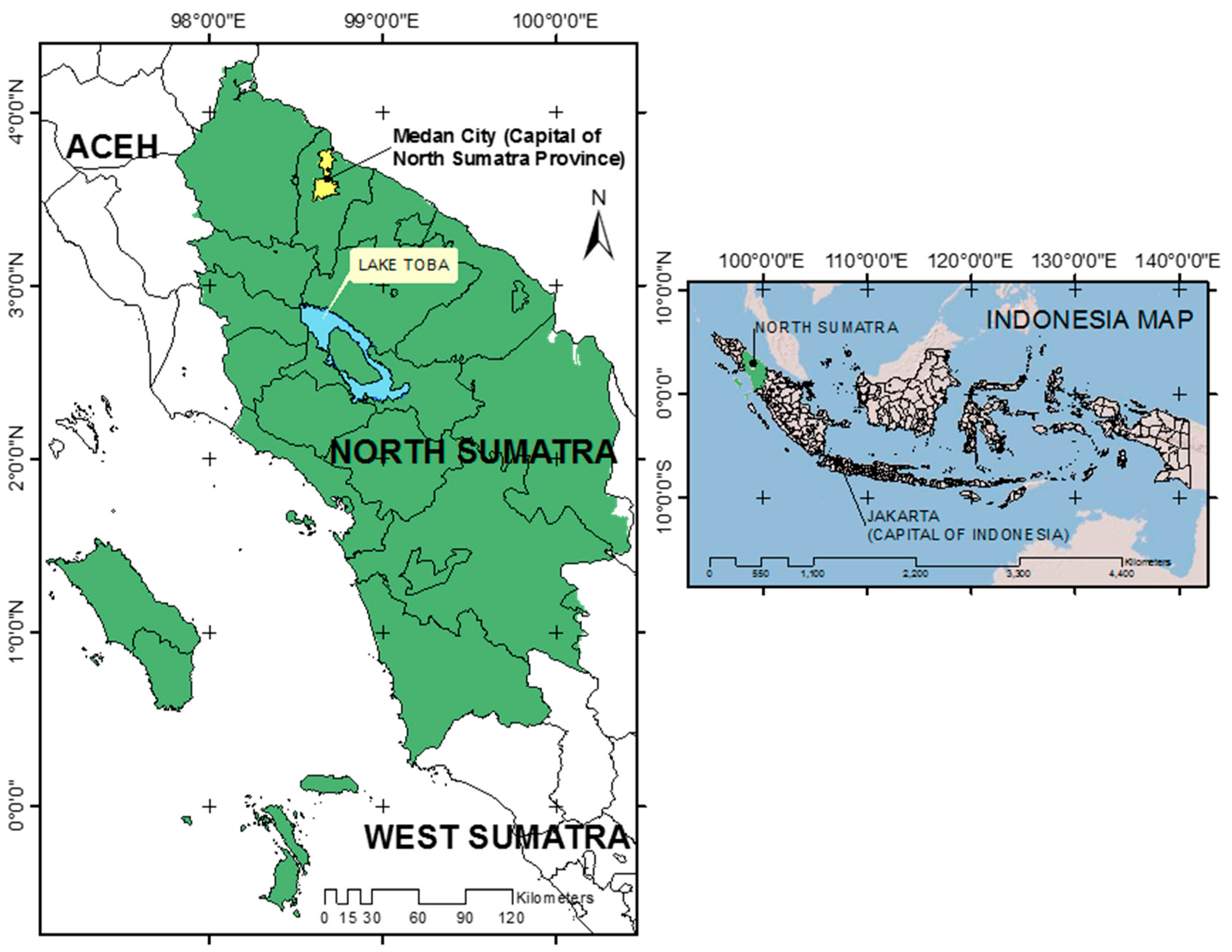
Figure 2.
Artificial-neural-network-based cellular automaton (ANN-CA) model structure for simulating LULC changes.
Figure 2.
Artificial-neural-network-based cellular automaton (ANN-CA) model structure for simulating LULC changes.
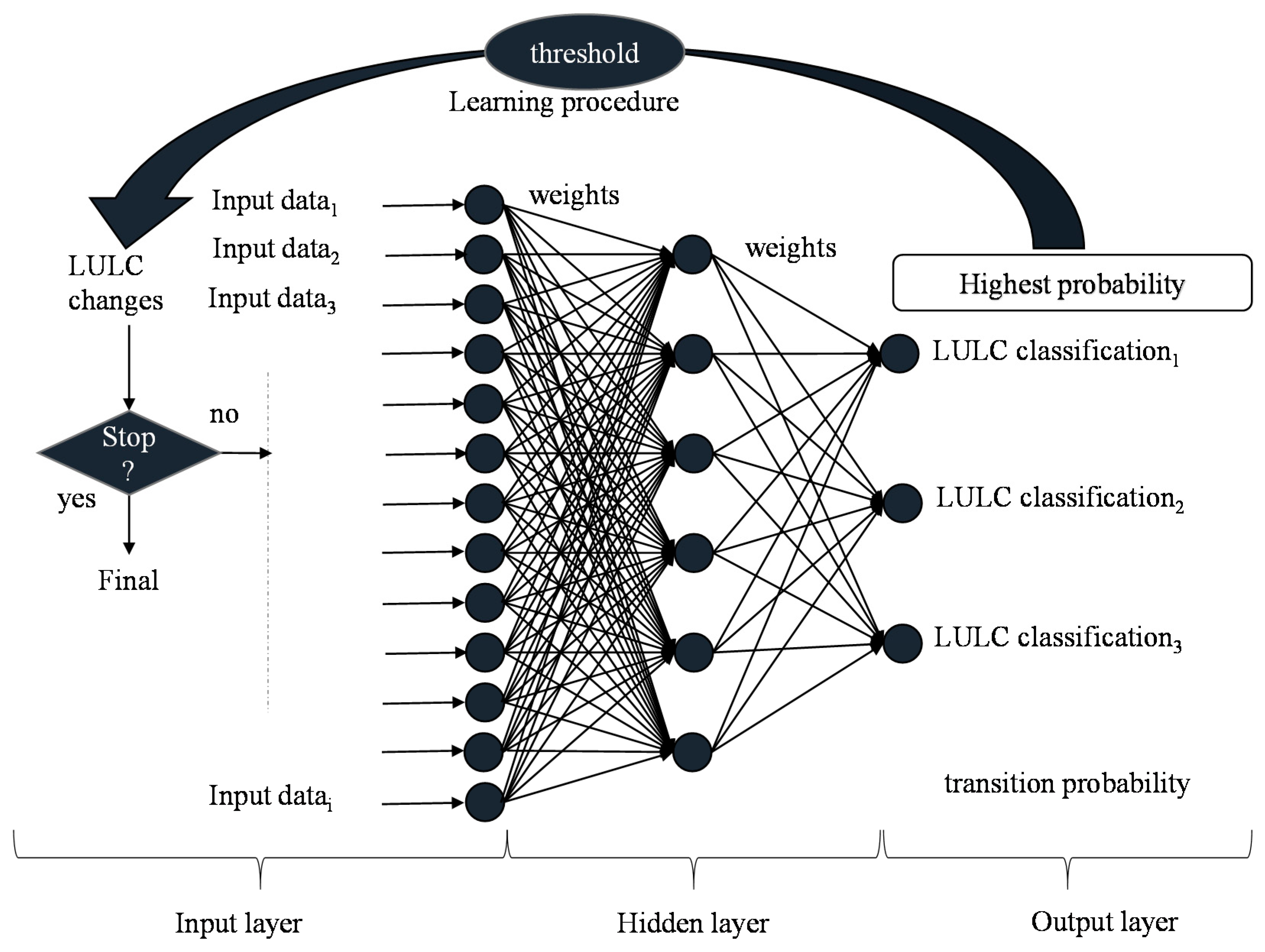
Figure 3.
Procedure for land use change analysis. The altitude and distance from the road are chosen for the exploratory map after the experiments by comparing the values of the Kappa coefficient and the percent of correctness from the other categories.
Figure 3.
Procedure for land use change analysis. The altitude and distance from the road are chosen for the exploratory map after the experiments by comparing the values of the Kappa coefficient and the percent of correctness from the other categories.
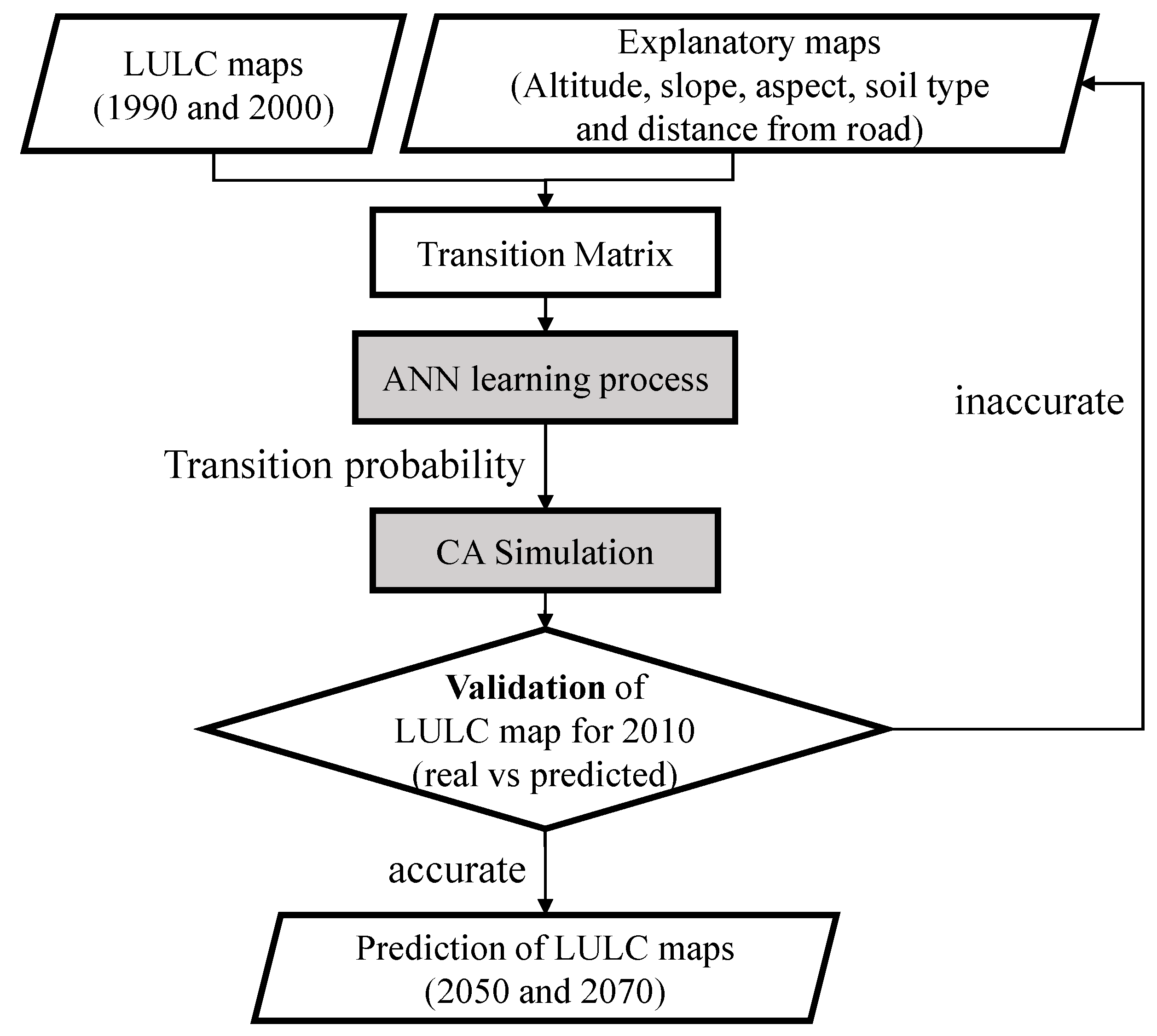
Figure 4.
(a) The altitude and (b) distance from road as the explanatory map for ANN-CA model. Altitude and distance from road are chosen as the explanatory map, since they and their combination result in higher scores for percent of correctness and Kappa index than the other criteria, such as slope, aspect, and urban density.
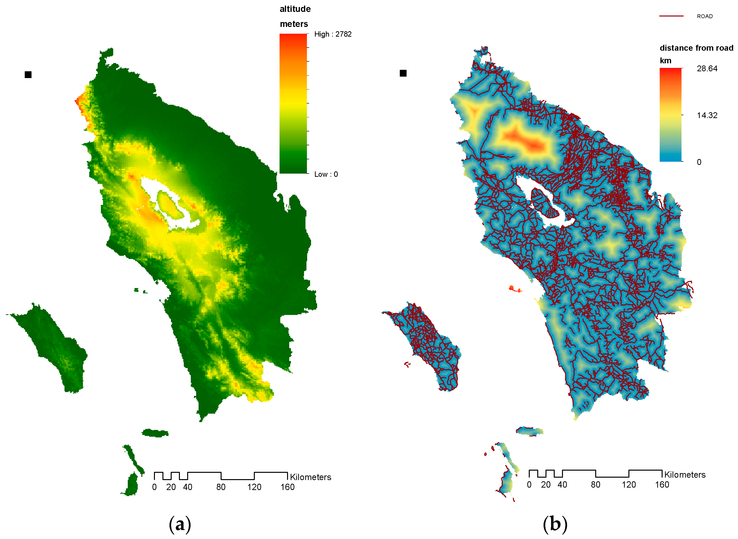
Figure 5.
Comparison between (a) the real and (b) the predicted LULC maps for 2010. The percentage of correctness is 87.28%, and the Kappa index is 0.83.
Figure 5.
Comparison between (a) the real and (b) the predicted LULC maps for 2010. The percentage of correctness is 87.28%, and the Kappa index is 0.83.
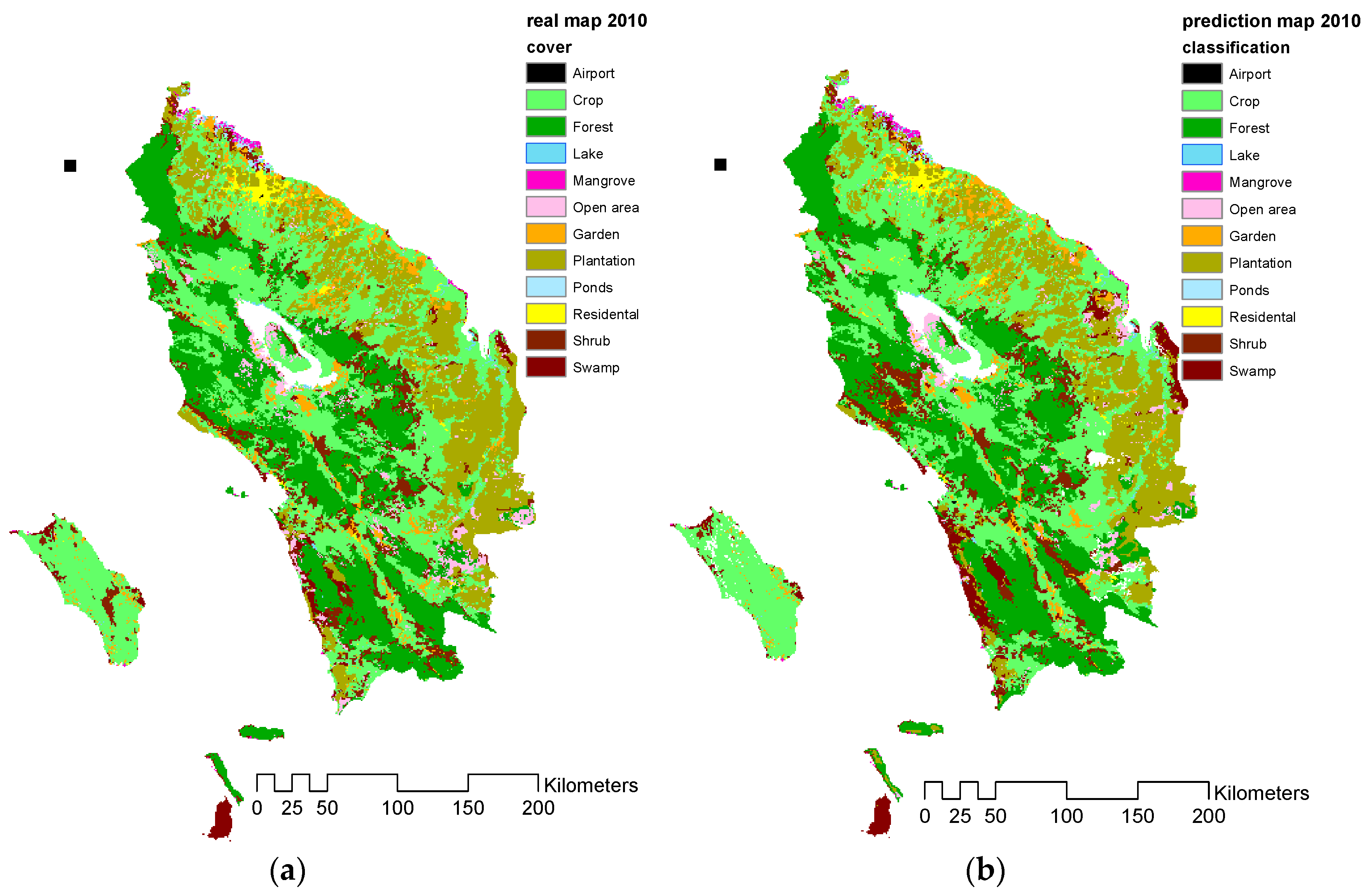
Figure 6.
The LULC classifications based on the suitable land use for Styrax sumatrana. (a) LULC for the year 2000, (b) the predicted LULC in the year 2050, and (c) the predicted LULC in the year 2070.
Figure 6.
The LULC classifications based on the suitable land use for Styrax sumatrana. (a) LULC for the year 2000, (b) the predicted LULC in the year 2050, and (c) the predicted LULC in the year 2070.

Table 1.
Summary of dataset, including digital elevation model (DEM), road map, soil type map, and land use and land cover (LULC) map used in this study.
Table 1.
Summary of dataset, including digital elevation model (DEM), road map, soil type map, and land use and land cover (LULC) map used in this study.
| Data | Criteria | LULC Simulation | Year | Description | Source | Data Format |
|---|---|---|---|---|---|---|
| DEM | Altitude | Exploratory map | 2017 | ASTER GDEM with 30 arc-sec spatial resolution | United State Geological Survey (USGS) (https://earthexplorer.usgs.gov/) | GeoTIFF |
| Slope | Exploratory map | |||||
| Aspect | Exploratory map | |||||
| Road map | Distance from the road | Exploratory map | 2000 | The main road map of North Sumatra | Ministry of Environment and Forestry, Indonesia | shp |
| Soil type | Soil type | Exploratory map | 2000 | A spatial soil type inventory (30 arc seconds) for year 2000 | Food and Agriculture Organization (FAO) (http://www.fao.org/soils-portal/soil-survey/soil-maps-and-databases/harmonized-world-soil-database-v12/en/) | TIFF |
| LULC map | LULC | Input map | 1990 | A satellite image from Landsat, USGS and LAPAN | Ministry of Environment and Forestry, Indonesia (http://webgis.dephut.go.id:8080/kemenhut/index.php/id/fitur/unduhan) | KML |
| 2000 | ||||||
| 2010 |
Table 2.
Twelve classifications for LULC maps.
| No | Classification | Description |
|---|---|---|
| 1 | Airport | The built area for transportation |
| 2 | Crop | The area for crop plants alone and with shrub plants |
| 3 | Forest | The area of primary, secondary and plantation forest |
| 4 | Lake | The area of large-scale water bodies |
| 5 | Mangrove | The area for primary and secondary mangrove forest |
| 6 | Open area | The barren area |
| 7 | Garden field | The area with square and near human settlement |
| 8 | Plantation | The area dominated by oil palm and rubber plant |
| 9 | Pond | The area of small-scale water bodies for fisheries |
| 10 | Residential | Transmigration and permanent residential area |
| 11 | Shrub | Shrub and juvenile plant area |
| 12 | Swamp | Primary and secondary swamp forest area |
Table 3.
Simulation results in terms of the percent of correctness and Kappa coefficient for explanatory data validation with difference combination of criteria.
Table 3.
Simulation results in terms of the percent of correctness and Kappa coefficient for explanatory data validation with difference combination of criteria.
| No | Criteria/Combination | % of Correctness | Kappa |
|---|---|---|---|
| 1 | Alt, road, urban | 86.59 | 0.83 |
| 2 | Alt, urban | 87.48 | 0.83 |
| 3 | Alt, road | 87.82 | 0.83 |
| 4 | Urban, road, | 85.8 | 0.81 |
| 5 | Alt, urban, road, soil type, aspect | 86.85 | 0.82 |
| 6 | Alt, urban, road, soil type, slope, aspect | 87.4 | 0.83 |
| 7 | Aspect, urban, slope | 87.28 | 0.83 |
Table 4.
Transition matrix of LULC classifications from 1990 to 2000 showing the changes in LULC for each classification. The values in the table vary from 0 to 1, with higher values indicating larger changes, except for the diagonal cells with high values, which depict no changes by remaining as the same category.
| Classification | 2000 | Sum | ||||||||||||
|---|---|---|---|---|---|---|---|---|---|---|---|---|---|---|
| Airport | Crop | Forest | Lake | Mangrove | Open Area | Garden | Plantation | Pond | Residential | Shrub | Swamp | |||
| 1990 | Airport | 1 | 0 | 0 | 0 | 0 | 0 | 0 | 0 | 0 | 0 | 0 | 0 | 1 |
| Crop | 0 | 0.96143 | 0.00046 | 0 | 0 | 0.00210 | 0.00631 | 0.02882 | 0.00018 | 0.00063 | 0.00004 | 0.00004 | 1 | |
| Forest | 0 | 0.00908 | 0.92400 | 0 | 0 | 0.01547 | 0.00013 | 0.04580 | 0 | 0 | 0.00493 | 0.00060 | 1 | |
| Lake | 0 | 0.00252 | 0 | 0.99748 | 0 | 0 | 0 | 0 | 0 | 0 | 0 | 0 | 1 | |
| Mangrove | 0 | 0.00521 | 0 | 0 | 0.81250 | 0.04167 | 0 | 0.00521 | 0.11458 | 0 | 0 | 0.02083 | 1 | |
| Open Area | 0 | 0.00417 | 0 | 0 | 0.00139 | 0.97153 | 0 | 0.02292 | 0 | 0 | 0 | 0 | 1 | |
| Garden | 0 | 0.02036 | 0 | 0 | 0 | 0.00750 | 0.93283 | 0.03108 | 0 | 0.00822 | 0 | 0 | 1 | |
| Plantation | 0 | 0.09766 | 0 | 0 | 0 | 0.01163 | 0 | 0.88856 | 0.00017 | 0.00009 | 0.00190 | 0 | 1 | |
| Pond | 0 | 0 | 0 | 0 | 0 | 0 | 0 | 0 | 1 | 0 | 0 | 0 | 1 | |
| Residential | 0 | 0 | 0 | 0 | 0 | 0 | 0.00571 | 0 | 0 | 0.99429 | 0 | 0 | 1 | |
| Shrub | 0 | 0.11184 | 0.00144 | 0 | 0 | 0.00497 | 0 | 0.05318 | 0 | 0 | 0.82833 | 0.00026 | 1 | |
| Swamp | 0 | 0.03147 | 0.00305 | 0 | 0.00025 | 0.05279 | 0.00685 | 0.15685 | 0.00812 | 0 | 0.03325 | 0.70736 | 1 | |
| Sum | 1.0 | 1.24374 | 0.92894 | 0.99748 | 0.81414 | 1.10765 | 0.95184 | 1.23242 | 1.12305 | 1.00322 | 0.86843 | 0.72909 | 12.0 | |
Table 5.
Comparison of changes between the predicted and the real maps in 2010 from the initial year in 2000. A positive value indicates the increase in the classification, whereas the negative values illustrate the decrease in the corresponding classifications. The differences between the predicted and the real maps in 2010 show the deviation values. The positive values indicate overestimations, while the negative values illustrate the underestimations of the changes.
| Classification | LULC Change Ratio | ||
|---|---|---|---|
| The Predicted (2010)–The Real (2010) | The Predicted (2010)–The Real (2000) | The Real (2010)–The Real (2000) | |
| Airport | 0.0001 | 0.0000 | −0.0001 |
| Crop | 1.1763 | 0.1986 | −0.9777 |
| Forest | 0.9279 | −0.5885 | −1.5164 |
| Lake | −0.0133 | −0.0173 | −0.0040 |
| Mangrove | 0.0740 | −0.0222 | −0.0962 |
| Open area | −0.8128 | −0.2665 | 0.5464 |
| Garden | −0.6965 | −0.0864 | 0.6102 |
| Plantation | −1.8071 | 1.1732 | 2.9804 |
| Ponds | −0.0438 | −0.0234 | 0.0203 |
| Residential | −0.0621 | −0.0456 | 0.0165 |
| Shrub | −0.2222 | −0.1752 | 0.0471 |
| Swamp | 1.4796 | −0.1468 | −1.6264 |
Table 6.
Percentage of land use land cover changes. A positive value indicates the increase in the classification, whereas the negative values illustrate the decrease in corresponding classifications.
Table 6.
Percentage of land use land cover changes. A positive value indicates the increase in the classification, whereas the negative values illustrate the decrease in corresponding classifications.
| Classifications | LULC Changes (%) | ||||
|---|---|---|---|---|---|
| 2070–2050 | 2070–2000 | 2050–2000 | 2000–1990 | 2010–2000 | |
| Airport | 0.0000 | −0.0001 | −0.0001 | 0.0001 | −0.0001 |
| Crop | −0.0012 | −1.2860 | −1.2848 | 1.3730 | −0.9777 |
| Forest | −0.0477 | −1.7256 | −1.6779 | −1.9777 | −1.5164 |
| Lake | 0.0000 | −0.0444 | −0.0444 | 0.0023 | −0.0040 |
| Mangrove | 0.0000 | −0.1084 | −0.1084 | −0.0817 | −0.0962 |
| Open area | −0.0098 | 0.3616 | 0.3714 | 0.9826 | 0.5464 |
| Garden field | 0.0073 | 0.3606 | 0.3532 | 0.0485 | 0.6102 |
| Plantation | 0.0330 | 4.1709 | 4.1379 | 2.1559 | 2.9804 |
| Pond | 0.0000 | 0.0081 | 0.0081 | 0.1031 | 0.0203 |
| Residential | −0.0012 | −0.1218 | −0.1206 | 0.0534 | 0.0165 |
| Shrub | 0.0220 | 0.1768 | 0.1547 | −1.2761 | 0.0471 |
| Swamp | −0.0024 | −1.7916 | −1.7891 | −1.3834 | −1.6264 |
© 2019 by the authors. Licensee MDPI, Basel, Switzerland. This article is an open access article distributed under the terms and conditions of the Creative Commons Attribution (CC BY) license (http://creativecommons.org/licenses/by/4.0/).
Share and Cite
MDPI and ACS Style
Saputra, M.H.; Lee, H.S. Prediction of Land Use and Land Cover Changes for North Sumatra, Indonesia, Using an Artificial-Neural-Network-Based Cellular Automaton. Sustainability 2019, 11, 3024. https://doi.org/10.3390/su11113024
AMA Style
Saputra MH, Lee HS. Prediction of Land Use and Land Cover Changes for North Sumatra, Indonesia, Using an Artificial-Neural-Network-Based Cellular Automaton. Sustainability. 2019; 11(11):3024. https://doi.org/10.3390/su11113024
Chicago/Turabian StyleSaputra, Muhammad Hadi, and Han Soo Lee. 2019. "Prediction of Land Use and Land Cover Changes for North Sumatra, Indonesia, Using an Artificial-Neural-Network-Based Cellular Automaton" Sustainability 11, no. 11: 3024. https://doi.org/10.3390/su11113024
Note that from the first issue of 2016, this journal uses article numbers instead of page numbers. See further details here.