The Underground Economy and Carbon Dioxide (CO₂) Emissions in China

Abstract

China aims to reduce carbon dioxide (CO₂) intensity by 40–45% compared to its level in 2005 by 2020. The underground economy accounts for a significant proportion of China’s economy, but is not included in official statistics. Therefore, the nexus of CO₂ and the underground economy in China is worthy of exploration. To this end, this paper identifies the extent to which the underground economy affects CO₂ emissions through the panel data of 30 provinces in China from 1998 to 2016. Many studies have focused on the quantification of the relationship between CO₂ emissions and economic development. However, the insights provided by those studies have generally ignored the underground economy. With full consideration of the scale of the underground economy, this research concludes that similar to previous studies, the inversely N-shaped environmental Kuznets curve (EKC) still holds for the income-CO₂ nexus in China. Furthermore, a threshold regression analysis shows that the structural and technological effects are environment-beneficial and drive the EKC downward by their threshold effects. The empirical techniques in this paper can also be applied for similar research on other emerging economies that are confronted with the difficulties of achieving sustainable development.

1. Introduction

During the past few decades, climate change has been a challenging problem all over the world [1]. As the primary greenhouse gas, carbon dioxide (CO₂) has been extensively recognized to be a common cause of global environmental issues [2]. China started to promote its industrialization and urbanization since 1978. The rapid industrialization and urbanization, however, have dramatically increased the CO₂ emissions in China [3]. Meanwhile, multiple developed countries have put pressures on China in climate change conferences [4]. Under such circumstances, at the Copenhagen climate agreement, the Chinese government set an ambitious target of reducing carbon intensity by 40–45% by 2020 compared to the level at 2005.

In some emerging and developing countries, considerable underground economies have fostered lots of environmental and climate problems to a rather large extent [5]. The underground economy, also called informal/black/shadow/non-observable economy, is commonly defined in the existing literature (e.g., Edgar [6] and Schneider [7]) as ‘all economic activities that contribute to the officially calculated/observed gross national product but are currently unregistered [5]’. Because the informal economy’s scale is not accounted for in official economic statistics, it tends to be higher than expected in China [8].

The hidden income of the urban household in China is not less than 4 trillion and 800 billion yuan [9] and the overall unobserved economy scale accounts for as much as 25%–49% of the gross domestic product (GDP) [10]. Therefore, if there exist pollution and energy-intensive industries among the underground economy, then, the underground economy can lead to nontrivial environmental issues (e.g., the increase of CO₂ and air pollution emissions) due to the comparatively loose environmental regulations in China [11]. Since China’s irrational industrial structure heavily relies on the secondary industry (mainly consisting of manufacturing and heavy industry) which is usually pollution- and energy-intensive, the underground economy may cause a surge in CO₂ emissions [12]. Besides, the underground economy can hinder environmental regulations and weaken the regulatory effects of developing countries [5]. Knowing these issues is helpful for policymakers to better coordinate CO₂ mitigation and the underground economic regulations. In this context, it is necessary to account for the underground economy when studying the relationship between the economic development and CO₂ emissions in China [13]. Additionally, the marginal effects of underground economic scale on carbon emissions level is worthy of estimation. Surprisingly, there is still a lack of empirical research on the underground economy–CO₂ nexus of China.

This study particularly contributes to the literature by overcoming the gaps of prior researches. This study’s main contribution is threefold. First, the study re-examines the EKC of China’s provincial-level CO₂ emissions by incorporating the underground economy into the analyzing framework through the random coefficients approach. To the best of the author’s knowledge, this is the first research work that has incorporated the underground economy into the analysis of CO₂ Kuznets curve, and found province-specific evidence supporting the income-CO₂ nexus. Second, the study empirically estimates the marginal effects of the underground economic scale on CO₂ emissions level by the threshold regression technique for the first time. This study clearly reveals a linear positive correlation between underground economic scale and CO₂ emissions in China. Third, through the threshold regression approach, the industrial structure and technical progress are verified as two of the driving factors for the ECK of CO₂ emissions in China. It is found that these two factors are nonlinearly related to the CO₂ emissions level depending on the personal income level. This is consistent with the theoretical expectation of EKC.

The remainder of the paper is organized as follows: Section 2 reviews past research on EKC and the underground economy. Section 3 introduces the theoretical foundation for this study. Section 4 describes the details of the variable, source of the data, empirical methodology and statistical inference strategies used in the paper. Section 5 illustrates and analyzes the model estimation results, then Section 6 further discusses the results. Section 7 concludes the whole research and presents suggestions.

2. Literature Review

2.1. EKC Hypothesis

Grossman and Krueger [14] introduced the EKC hypothesis, suggesting the existence of an inverse U-shaped relationship between pollutants and economy growth/income. Stern [15] and Holtz-Eakin and Selden [16] then testified the EKC hypothesis by CO₂ emissions data. Zhang and Lin [17] explored the EKC and evaluate the urbanization’s effectiveness on CO₂ emissions in the eastern, western, and central parts of China. Moreover, Kaika and Zervas [18,19] argued that other than increasing income, technical progress and international trade are also driving factors for the CO₂ EKC. Yin et al. [20] verified the beneficial effects of technological advancement and environmental regulations on CO₂ emission reduction. They concluded an inverse U-shape CO₂ EKC in China. In recent years, advance methods were also adopted for EKC studies. Taskin and Zaim [21] examined CO₂ emissions in 52 countries from 1975 to 1990 through nonparametric regression. They claimed an inverted N-shape relationship between personal income and CO₂ emissions with double turning points: $5000 and $12,000 per capita. Maddison [22] explored the EKCs for carbon, sulfur and nitrogen dioxide as well as volatile organic compounds in 135 countries. He detected the spatial interactions between the emissions of local and adjacent countries with spatial statistic tools. By the spatial panel data method, Zheng et al. [23] and Kang et al. [24] verified an inversely N-shaped EKC for CO₂ emissions in China. Similarly, Zhou et al. [25] and Ge et al. [26] testified inverse N-shape EKCs for sulfur dioxide and nitrogen oxide emissions in China using spatial panel data techniques. Xu et al. [27] investigated the correlations among income, household fuel consumption, and CO₂ emissions through the EKC model at both the regional and national level and validate the EKC assumption in China. Haseeb et al. [28] estimated the impact of economic growth, financial development and other socio-economic factors on CO₂ emissions in the presence of the EKC framework for BRICS economies, new evidence was found to support the EKC hypothesis in BRICS economies.

Like any other theory, the EKC hypothesis has raised critiques and doubts among academia. Different opinions and critiques mainly focus on the shape, the sample and the adopted methods of EKC studies.

Some scholars argued against the EKC of the classical inverse U-shape, they believed that the inverse U-shape does not hold when a longer time interval is evaluated for the curve [29]. For instance, Millimet et al. [30] claimed that the inverse U-shaped EKC was essentially derived from an N-shaped EKC. They further elaborated their idea: Environmental deterioration increases in the early stage of the development in a country. After reaching the threshold level of income, the deterioration decreases and then increases with income. Taskin and Zaim [21] found an inverted N-shaped nexus between CO₂ emissions and economic growth for 52 countries from 1975 to 1990 by the nonparametric regression approach. In addition, Zheng et al. [23] and Kang et al. [24] applied the spatial panel data approach and concluded an inverted N-shaped relationship between CO₂ emissions and economic growth in China.

Many of the early EKC research works made the conclusion of a unique EKC existing among different countries/regions merely based on the investigation of cross-sectional data, however, cross-sectional data has been criticized for its invalidity on EKC hypothesis verification [31,32,33]. Because as the economy keeps growing, a group of regions may go through environmental improvement, while other regions (in the same sample population) experience environmental degeneration. An inverted-U shape EKC can be derived from the cross-sectional regression on the sample that mixed these two different groups. Nevertheless, such an inverse U-shape curve does not depict the path of any group of this sample [34].

Bradford et al. [35] hold the view that personal income and per capita pollution emissions, as well as the logarithmic transformations of them, are usually non-stationary unit root processes. Therefore, nonstationary econometric techniques (i.e., panel unit root and panel co-integration tests) were adopted for the verification of EKC with panel data [36,37,38,39]. However, the pre-assumption for the validity of panel unit root tests (i.e., independent and identically distributed sampling) is usually not practical in most empirical research. Nonlinear transformations would change the stochastic characters of a unit root process, therefore, the commonly applied logarithmic transformations of the dependent and independent variable in the unit root process are problematic [40]. Prior studies generally ignored these issues when empirically using panel unit root tests [34].

2.2. The Underground Economy and Its Environmental Impacts

Kostakis [41] examined the underground economy and corruption’s impacts on private consumption and conclude that the underground economy and corruption could be substitutes concerning its effect on real consumption growth of individuals. Hajilee et al. [42] analyzed the impact of the underground economy on the financial market in the short- and long-run by using the annual data (1980–2013) for 18 merging economies. They argue that the underground economy has significant asymmetric impacts on the financial market in the short-run and no effects in the long-run.

There is only a limited number of works in the literature that have studied the relationship between the underground economy and environmental quality, and the previous work mainly focused on theoretical construction. Scholars generally believe that the underground economy can worsen environmental pollution. After analyzing the issues of polluting informal sectors of Mexico, Blackman et al. [43] argued that owing to the wide application of low technology, the informal sectors are major sources of pollution and the size of pollution emissions in these underground economic sectors is significantly environment-beneficial. Biswas et al. [5] developed a theoretical model that incorporates the environmental pollution, corruption and underground economy into an integrated framework to reveal the mechanism of how the underground economy aggravates environmental deterioration under a certain level of corruption. They found that the control of corruption can mitigate the impact of the underground economy on environmental pollution. After scrutinizing the informal economy’s effectiveness on multiple pollution indices by the annual data of Turkey, Elgin and Oztunali [13] argued that the small-scale informal economy always has a relatively higher pollution level and vice versa.

Other extant works of literature also explored and verified that pollutant emissions are closely related to the underground economy (e.g., Baksi and Bose [44] and Croitoru and Sarraf [45]).

3. Theoretical Framework

This section introduces the theoretical framework on which the research is based.

3.1. EKC Model

Originally, the Environmental Kuznets Curve is an empirical hypothesis that depicts an inverse U-shape curve for the nexus of environmental quality and economic development. More specifically, at an early stage of the development, production expansion and wealth accumulation are preferred over environmental quality, thus, resource consumption, pollution emissions and environment degeneration emerge as economic growth. After reaching the threshold level of development, the environmental quality begins to improve [14]. The reason for the environmental improvement might be the pollution reduction, technological advancement, industrial structural upgrade and the public’s demand for a better environment to be promoted by economic development [22]. Generally, when the wealth has reached a specific level, the public tends to trade economic efficiency for environmental quality through technological, economic and political ways [46].

The following econometric model is commonly applied to empirically verify the existence of EKC and the shape [47]:

$$Y=\alpha +{\beta }_{1}X+{\beta }_2{X}^2+{\beta }_3{X}^3+{\beta }_{4}Z+\epsilon$$

(1)

where, Y is the indicator of environmental quality, X is the economic development measured by per capita GDP (Gross Domestic Product), and Z is the set of control variables that represent other influential factors of the environment. This polynomial function offers an empirical tool for testing and estimating EKC: (1) β₁ = β₂ = β₃ = 0: Y and X are not related; (2) β₁ > 0, β₂ = β₃ = 0: a positive relationship between Y and X; (3) β₁ < 0, β₂ = β₃ = 0: a negative relationship between Y and X; (4) β₁ > 0, β₂ < 0 and β₃ = 0: an inverse-U shape nexus (i.e., the classical EKC); (5) β₁ < 0, β₂ > 0 and β₃ = 0: a U-shaped nexus; (6) β₁ < 0, β₂ > 0 and β₃ < 0: an inversely N-shaped curve; (7) β₁ > 0, β₂ < 0 and β₃ > 0: an N-shape curve.

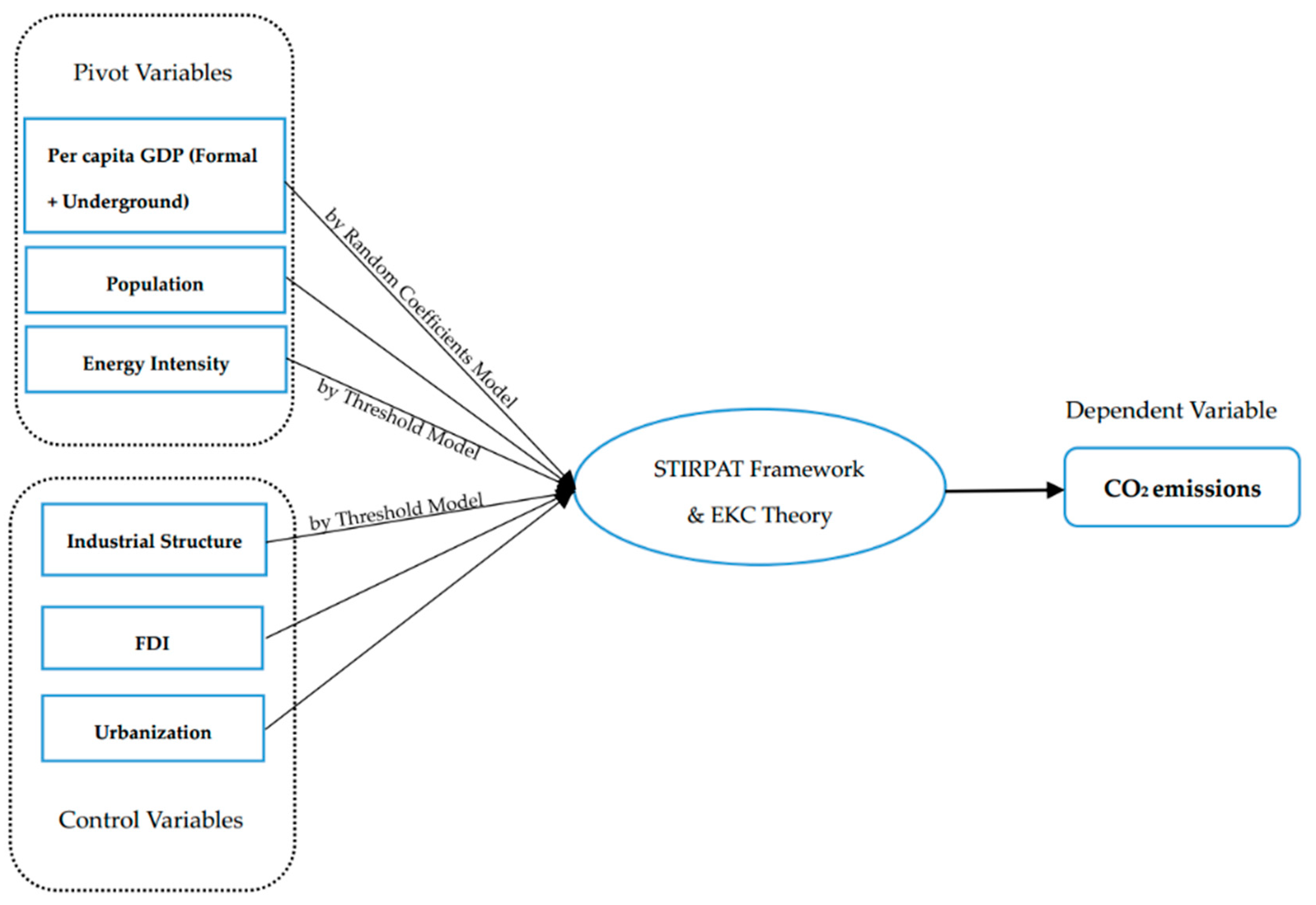
3.2. STIRPAT Model

Dietz and Rosa [48] developed a stochastic version of the IPAT (Impact, Population, Affluence, and Technology) concept, which is known as the STIRPAT model. Later on, York et al. [49] refined the STIRPAT framework and expressed it by the empirical form:

$$I_i={\alpha }_i{P}_i^b{A}_i^c{T}_i^d{\epsilon }_i$$

(2)

In Equation (2), I indicates the environmental impact, and P, A, and T represent the population, economic development and technology influences, respectively. The subscript i indicates the ith observation (usually regions) and the value of a variable varies across observations. ε is the random error term that enables statistical estimation for the coefficients α, b, c and d in the empirical function.

According to the purpose of this study, the total per capita GDP, abbreviated as GDPT (GDPT = per capita GDP + per capita informal GDP (abbreviated as GDPN)), is defined as the index of the economic development level; as routine, energy intensity (EI, energy consumption per unit of output) is used to reflect the technology impacts [46]; the annual resident population size is used as the indicator of the population effects; Environmental impact is indexed by the amount of CO₂ emissions.

Besides, China has maintained the largest foreign capital scale for many years among developing countries. The continuous injection of foreign direct investment (FDI) promotes the technical and management level of local enterprises and stimulates the economic growth as well as export trade of China [50]. Meanwhile, the impact of FDI on Chinas pollution and environmental quality has been paid more attention by scholars (e.g., Wang and Jin [51]; Bao et al. [52] and Dean et al. [53]). Since 2015, the Chinese government started to promote the optimization of the industrial structure for energy-saving and emission-reduction purpose in the long term. The gradually optimized industrial structure is believed to be environment-beneficial in China. The transmission of production factors between industries would take effects on the emissions level [47,54]. Other than that, China has been boosting the infrastructure construction in urban areas and sprawling its cities for decades, thus urbanization is another significant influencing factor of environmental quality [36,55,56]. Therefore, the analytical framework also incorporates the effects of FDI (fdi), industrial structure (str) and urbanization (urb).

The STIRPAT model is highly flexible to various functional forms and permits the addition of other variables [49] to control for the impacts of factors other than development, population and technology. Thus, the logarithmic extended STIRPAT model is adopted to satisfy the needs of the study:

$$\ln C{O}_2=b\ln GDPT+{\beta }_1\ln P+{\beta }_2\ln EI+{\beta }_{3}fdi+{\beta }_{4}str+{\beta }_{5}urb+\epsilon$$

(3)

$$\ln C{O}_2=b_1\ln GDPT+b_2{(\ln GDPT)}^2+{\beta }_1\ln P+{\beta }_2\ln EI+{\beta }_{3}fdi+{\beta }_{4}str+{\beta }_{5}urb+\epsilon$$

(4)

$$\ln C{O}_2=b_1\ln GDPT+b_2{(\ln GDPT)}^2+b_3{(\ln GDPT)}^3+{\beta }_1\ln P+{\beta }_2\ln EI+{\beta }_{3}fdi+{\beta }_{4}str+{\beta }_{5}urb+\epsilon$$

(5)

The combined use of quadratic and cubic income terms in the model enables a more thorough investigation of CO₂ EKC. In the STIRPAT framework, linear and higher order terms of lnGDPT, lnP and lnEI are the pivot variables while other independent variables can be seen as control variables. In sum, the theoretical framework with its characteristics is shown in Figure 1.

4. Methodology and Data (Variables)

4.1. Measuring the Underground Economy Scale

Activities of the underground economy are carried out with secretive manners and not recorded by official statistics, so it is difficult to accurately explore these activities. Despite various difficulties, different methods have been developed by some scholars to quantitatively evaluate the scale/size of the underground economy. The main applicable accounting methods are the currency demand method and production factor method. Although the currency demand method is a comparatively ideal method to measure the scale of China’s underground economy [57], it is unable to estimate the scale at the provincial level. Thus, this study adopts the production factor method [58] to measure the underground economy’s scale in each province.

The informal economy is not strictly isolated from the formal economy. The income from the formal economic sector can be used to purchase products in the informal economic sector, while gray income from the informal sector may be legally consumed. Based on this connection, the income received from the underground economy can be indirectly obtained. Therefore, the total income in the informal economic sector can be inferred by the difference between the income and expenditure of the whole society. Further, once the share of informal income in the underground economy scale is known, the scale of the underground economy can be inferred (it is assumed that the informal economic and the formal economic sectors are similar in terms of factors of production structure) [57,58].

According to the principle of macroeconomic accounting [58]:

$$I=C+S$$

(6)

Here, I, C and S refer to income, consumption, and savings in an economy. Further [58],

$$IU=E+AS-(UI·UP+RI·RP)$$

(7)

In Equation (7), IU indicates the total income in the underground economic sector; E, AS, UI, UP, RI and RP indicate the total household expenditure, annual increase of residents’ savings, per capita income of urban residents, urban population, per capita income of rural residents and rural population respectively [58].

Because the production factor method assumed that the factors of production structures in the informal economic and the formal economic sectors are similar, the income-GDP ratio of underground economic sector equals the income-GDP ratio of the formal economic sector [57,58] which can be expressed by Equation (8):

$$\frac{IU}{NGDP}=\frac{IN}{GDP}$$

(8)

where NGDP, IN, and GDP are the scale of the underground economy (the unobserved GDP), income in the formal economic sector and the formal economic scale (the official real GDP) respectively. The official statistics of residents’ consumption expenditures, saving and income, as well as provincial GDP, are easily accessible, thus the scale of underground economic scale can be directly estimated through Equations (7) and (8).

4.2. The Random Coefficients Model

Most of the EKC studies have restricted the coefficients of per capita income to be the same for every observation (countries, provinces, cities, etc.) because of the application of the traditional cross-section/penal data model. In the context of the great diversity of political, social, geographical and economic situations across regions, this restriction hardly makes any sense. The adoption of the random coefficients model can overcome the heterogeneous issue. As depicted by Equation (9) [59]:

$$y_{it}=x_{it}^{\prime }{\beta }_i+{\epsilon }_{it}=x_{it}^{\prime }(\beta +{\upsilon }_i)+{\epsilon }_{it}=x_{it}^{\prime }{\beta }_i+(x_{it}^{\prime }{\upsilon }_i+{\epsilon }_{it})$$

(9)

where ${\beta }_i=\beta +{\upsilon }_i$ and ${\beta }_i=({\beta }_0,{\beta }_{i1},\dots ,{\beta }_{ik})$ are assumed subjecting to the same distribution. υ_i is a random vector that is subject to $E({\upsilon }_i|x_i)=0$. β is a constant parameter vector that provides the average CO₂-income nexus. Since ${\beta }_{i1},\dots ,{\beta }_{ik}$ can vary across regions, the nexus of CO₂-income experienced by individual regions can be different from the average relationship [59].

4.3. The Threshold Regression

The threshold regression model is designed to capture the structural break in the relationship between economic variables. The relationship can be described by a nonlinear model of individual observations which could be divided into different classes based on the value of the observed threshold variable. Consider a general single-threshold model [60]:

$$y_{it}={\beta }_1^{\prime }{X}_{it}I(q_{it}\le \gamma )+{\beta }_2^{\prime }{X}_{it}I(q_{it}>\gamma )+Z_{it}{\beta }_3^{\prime }+{\mu }_i+{\epsilon }_{it}$$

(10)

where the I(·) is the indicator function and γ is the threshold parameter that divides the equation into two ‘regimes’. The regimes are distinguished by different regression slopes, β₁ and β₂. X_it and Z_it are regime dependent and regime independent variables. An alternative compact way of writing Equation (10) is $y_{it}=\{\begin{array}{c}{\beta }_1^{\prime }{X}_{it}+{\mu }_i+{\epsilon }_{it},q_{it}\le \gamma \\ {\beta }_2^{\prime }{X}_{it}+{\mu }_i+{\epsilon }_{it},q_{it}>\gamma \end{array}$ [60].

The dependent variable y_it and the threshold variable q_it are scalers, and the independent variable X_it and Z_it are k-dimensional vectors. μ_i is the individual effect and ε_it is the error term.

The threshold parameter γ can be estimated by least-squares, which is easy to achieve by minimizing the residual sum of squares (RSS). One can search through a subset of the threshold variable q_it and the estimator of γ is the value which minimizes the RSS. Given γ, the slope parameter β can be estimated by ordinary least-squares (OLS) [60]. Specifically, the average of Equation (10) over time (index of t) is [60]

$${\overline{y}}_i^{}={\beta }_{}^{\prime }{\overline{X}}_i^{}(\gamma )+{\beta }_3^{\prime }{\overline{Z}}_i^{}+{\mu }_i+{\overline{\epsilon }}_i^{}$$

(11)

where ${\overline{y}}_i=\frac{1}{T}{\displaystyle {\sum }_{t=1}^T{y}_{it}},{\overline{\epsilon }}_i=\frac{1}{T}{\displaystyle {\sum }_{t=1}^T{\epsilon }_{it}},{\overline{Z}}_i=\frac{1}{T}{\displaystyle {\sum }_{t=1}^T{Z}_{it}}$ and ${\overline{X}}_i(\gamma )=\frac{1}{T}{\displaystyle {\sum }_{t=1}^T{X}_{it}}(\gamma )=\{\begin{array}{c}\frac{1}{T}{\displaystyle {\sum }_{t=1}^T{X}_{it}}I,q_{it}\le \gamma \\ \frac{1}{T}{\displaystyle {\sum }_{t=1}^T{X}_{it}}I,q_{it}>\gamma \end{array}$.

Taking the difference between Equations (10) and (11) produces [60]

$$y_{it}^{*}={\beta }_{}^{\prime }{X}_{it}^{*}(\gamma )+{\beta }_3^{\prime }{Z}_{it}^{*}+{\epsilon }_{it}^{*}$$

(12)

Here, $y_{it}^{*}=y_{it}^{}-{\overline{y}}_i,X_{it}^{*}(\gamma )=X_{it}^{}(\gamma )-{\overline{X}}_i(\gamma ),Z_{it}^{*}=Z_{it}^{}-{\overline{Z}}_i$ and ${\epsilon }_{it}^{*}={\epsilon }_{it}^{}-{\overline{\epsilon }}_i$. Then the estimation of $\beta (\gamma )$ can be obtained by OLS and furthermore, the ${\widehat{\epsilon }}^{*}(\gamma )$ (estimator of ${\epsilon }^{*}$) can be derived.

It is critical to test if the threshold is statistically significant in the empirical analysis. The null hypothesis of the test is that no threshold exists, namely, the difference between β₁ and β₂ is statistically insignificant (H₀: β₁ = β₂).

The test of H₀ is conducted by a likelihood ratio of a Chi-square distribution with the bootstrap procedure [61]. And so on, one can deal with the double and multiple-threshold regressions in the same way.

4.4. Measuring CO₂ Emissions from Energy Consumption

Fossil fuel combustion and electric power consumption are the main sources of CO₂ emissions from human activities. Due to the lack of direct monitoring and measuring means, a majority of the research measures the CO₂ emissions of China through the method provided by the Intergovernmental Panel on Climate Change (IPCC) [62]. This method calculates the CO₂ emissions through energy consumptions:

$$C{O}_2=\frac{44}{12}{\displaystyle \sum _{i=1}^{7}E{F}_{i}Con{v}_{i}Con{s}_i}$$

(13)

where the values of i (1–7) denote 7 kinds of energy including raw coal, coke, fuel oil, diesel, kerosene, gasoline, and electricity. The fraction 44/12 is the molar ratio of CO₂ to carbon. The Cons_i indicates the consumption of i-th energy which needs to be converted to its standard coal equivalent by multiplication with the conversion coefficient (Conv_i), while EF_i denotes the carbon emission factor of i-th energy.

Table 1. The CO₂ emission factors and standard coal equivalent conversion coefficients.

Energy Type	Raw Coal	Coke	Fuel Oil	Diesel	Kerosene	Gasoline	Electricity
Emission factor	0.7559	0.8550	0.6185	0.5921	0.5714	0.5538	0.2720
Conversion coefficient (tce/t)	0.7143	0.9714	1.4286	1.4571	1.4714	1.4714	-

Note: The unit of CO₂ emission factor of electricity is 10,000 tC/kWh. Resource: IPCC [62].

lists all the carbon emission factors and the conversion coefficients for i-th energy.

4.5. Variables and Data Resource

This research estimates the impacts of the underground economic scale on CO₂ emissions and investigates the CO₂ EKC with the inclusion of the underground economy in China, via a panel of 19 years (1998–2016) of provincial data (the data of Tibet autonomous region, Taiwan province, Hong Kong and Macau special administrative regions are not available). The author takes the indicators of proportion of urban population, ratio of FDI to GDP, real per capita GDP, and population size to reflect the urbanization, foreign capital inflow, economic development, and population. The proportion of the secondary industry [20,63,64] and energy intensity [46] are defined as the indicators of economic structure and technology impacts.

Every kind of energy consumption and the standard coal consumption (kg of coal equivalent, used for calculating energy intensity) were obtained from the China Energy Statistical Yearbook. FDI and the secondary industry output were collected from the China City Statistical Yearbook in the EPS data bank. Personal income, GDP, urban population and total population were obtained from the China Statistical Yearbook. The per capita GDP was converted into the 1995 constant price.

As for the data used to calculate the scale of the underground economy, the total income of urban personnel in 1998–2001, 2015 and 2016 are obtained from the EPS databank, residents’ savings deposit of 1998–2001, 2015 and 2016 are obtained from the EPS data bank, and these indicators of 2002–2014 are obtained from the National Statistics Bureau of China [65]. The total consumption expenditure of residents is also obtained from the National Statistics Bureau of China. Per capita income of rural residents is obtained from the China Labor Statistical Yearbook; the rural population is obtained from the China City Statistical Yearbook. Definitions and descriptive statistics of the variables are listed in

Table 2. The definitions and descriptive statistics of the variables.

Variable	Definition (unit)	Mean	Std. Dev.	Min	Max
lnGDPT	Total (underground + formal) per capita GDP (100 yuan)	5.435	0.845	3.354	7.596
lnGDPN	Underground per capita GDP (100 yuan)	4.188	0.981	1.286	6.762
fdi	Ratio of FDI to GDP (%)	2.765	2.698	0.001	21.188
str	Proportion of secondary industry (%)	45.325	7.853	19.262	59.045
lnPOP	Total Population (10 thousand)	8.143	0.763	6.221	9.306
urb	Proportion of urban population (%)	47.414	15.621	21.890	89.600
lnEI	Energy intensity (tons of coal equivalent/billion yuan)	9.639	0.506	8.669	10.928
lnCO2	Carbon dioxides emissions (10,000 tons)	10.155	0.894	6.904	12.030

Note: lnGDPT, lnGDPN, lnPOP, lnEI and lnCO₂ are processed with natural logarithm transformation. GDPN is calculated through the production factor method introduced in Section 4.1. Per capita CO₂ emissions is the other commonly used indicator. The population is one of the independent variables in all the regression models so there will be no differences in the estimates of all parameters whether the study uses the per capita or total CO₂ emissions as the indicator.

.

According to the study purpose, total per capita GDP (including its powers), underground per capita GDP, energy intensity and secondary industry proportion are the core explanatory variables, and the remaining variables are control variables in all empirical models.

5. Results

5.1. The EKC Estimation

In the EKC studies, if the per capita GDP and its’ quadratic and cubic terms are included as the independent variables of the traditional panel data regression model, then each region (province/city) will have the same shaped EKC, while the intercept (fixed effects) will enable the EKC to shift up and down vertically for different regions. However, there is no reason to assume that different regions in China are experiencing the same CO₂-income relationship, given the differences in socio-economics, culture, geography, climate, etc. that exist across these regions. Therefore, this study adopts an alternative and less restrictive random coefficients model that shows the cross-provincial heterogeneities in the shape of the income-CO₂ nexus.

All the empirical results in this study are generated through Stata 15.

Table 3. The random coefficients model results.

Dependent Variable: lnCO2	Cubic Model	Quadratic Model	Linear Model
lnGDPT	−9.430 ***	0.249	0.329 ***
	(−2.92)	(0.76)	(4.68)
(lnGDPT)2	1.819 ***	0.008
	(2.90)	(0.24)
(lnGDPT)3	−0.113 ***
	(−2.77)
fdi	−0.016 *	−0.01	−0.008
	(−1.74)	(−0.78)	(−0.60)
str	0.014 ***	0.018 ***	0.016 ***
	(3.43)	(4.26)	(3.69)
lnPOP	0.631	0.410	0.386
	(0.82)	(0.42)	(0.45)
urb	0.040 ***	0.037 ***	0.037 ***
	(3.91)	(3.65)	(4.27)
lnEI	0.379 ***	0.431 ***	0.466 ***
	(3.02)	(3.46)	(4.39)
Test of parameter constancy (χ2)	17,749.03 ***	15,448.34 ***	14,487.28 ***
Observations	570	570	570

T-statistics in parentheses, * p < 0.10, ** p < 0.05, *** p < 0.010. The linear, quadratic and cubic specifications are based around Equations (3)–(5) respectively.

presents estimates of Equations (3)–(5) by the random coefficients approach. The linear, squared and cubic income coefficients in the cubic model are highly significant, thus the cubic model specification is superior to the quadratic and linear specifications because the linear and quadratic models are naturally nested in the cubic model. The χ²-statistics (test of parameter constancy with the null hypothesis: β_1j = β_2j = … = β_mj) overwhelmingly reject that the independent variables are the same for each province. Hence, in order to know the extent to which such an “average” nonlinear (cubic) nexus is meaningful/representative, the province-specific estimations were conducted (shown in Appendix

Table A1. The province-specific coefficients (the cubic model of Table 3).

	lnGDPT	(lnGDPT)2	(lnGDPT)3		lnGDPT	(lnGDPT)2	(lnGDPT)3
Beijing	−9.211 **	1.282 *	−0.059	Henan	−1.066	0.388	−0.037
	(−2.27)	(1.87)	(−1.54)		(−0.19)	(0.34)	(−0.47)
Tianjin	−0.127	0.138	−0.012	Hubei	−7.089	1.510	−0.100
	(−0.04)	(0.24)	(−0.38)		(−1.39)	(1.47)	(−1.45)
Hebei	−16.347 **	3.232 **	−0.206 **	Hunan	−0.761	0.151	−0.006
	(−2.41)	(2.43)	(−2.36)		(−0.14)	(0.14)	(−0.08)
Shanxi	−2.352	0.552	−0.041	Guangdong	−8.852 **	1.647 **	−0.099 **
	(−0.41)	(0.47)	(−0.53)		(−1.96)	(2.14)	(−2.27)
Inner Mongolia	−9.219 **	1.836 **	−0.110 **	Guangxi	3.374	−0.591	0.037
	(−2.12)	(2.17)	(−2.04)		(0.68)	(−0.58)	(0.54)
Liaoning	−40.051 ***	7.308 ***	−0.442 ***	Hainan	−13.229 **	2.440 *	−0.141 *
	(−7.48)	(7.74)	(−7.94)		(−1.95)	(1.87)	(−1.69)
Jilin	−14.965 ***	2.894 ***	−0.183 ***	Chongqing	−20.888 ***	3.913 ***	−0.239 ***
	(−2.59)	(2.62)	(−2.62)		(−3.16)	(3.12)	(−2.99)
Heilongjiang	−6.408	1.219	−0.071	Sichuan	−1.644	0.385	−0.030
	(−0.84)	(0.85)	(−0.79)		(−0.31)	(0.36)	(−0.41)
Shanghai	−0.920	0.157	−0.008	Guizhou	−6.496	1.605 *	−0.115 *
	(−0.39)	(0.44)	(−0.42)		(−1.52)	(1.73)	(−1.78)
Jiangsu	−8.606 *	1.460 *	−0.076 *	Yunnan	−7.414	1.779	−0.133
	(−1.94)	(1.88)	(−1.68)		(−1.21)	(1.45)	(−1.64)
Zhejiang	−13.700 ***	2.454 ***	−0.141 ***	Shaanxi	−16.758 ***	3.414 ***	−0.230 ***
	(−3.60)	(3.81)	(−3.89)		(−4.68)	(4.61)	(−4.54)
Anhui	−10.857 **	2.231 **	−0.148 **	Gansu	11.129 ***	−2.469 ***	0.185 ***
	(−2.44)	(2.45)	(−2.45)		(3.38)	(−3.34)	(3.40)
Fujian	−14.921 **	2.670 **	−0.154 **	Qinghai	−20.965 ***	4.178 ***	−0.267 ***
	(−2.48)	(2.49)	(−2.42)		(−3.85)	(3.76)	(−3.58)
Jiangxi	5.052	−1.151 *	0.085 *	Ningxia	−2.108	0.711	−0.060
	(1.56)	(−1.66)	(1.73)		(−0.35)	(0.59)	(−0.74)
Shandong	−11.244 **	2.187 ***	−0.138 ***	Xinjiang	−36.255 ***	7.051 ***	−0.449 ***
	(−2.39)	(2.62)	(−2.75)		(−5.01)	(4.98)	(−4.85)

T-statistics in parentheses, * p < 0.10, ** p < 0.05, *** p < 0.010. Estimations of other variables (fdi, str, lnPOP, urb, and lnEI) are omitted.

and

Table A2. The province-specific coefficients (cubic model with only pivot variables, M4 of Table 6).

	lnGDPT	(lnGDPT)2	(lnGDPT)3		lnGDPT	(lnGDPT)2	(lnGDPT)3
Beijing	−21.546 ***	3.648 ***	−0.203 ***	Henan	−12.340 ***	2.821 ***	−0.199 ***
	(−3.73)	(3.85)	(−3.92)		(−2.71)	(3.02)	(−3.12)
Tianjin	−9.420 **	1.725 **	−0.099 ***	Hubei	−22.595 ***	4.496 ***	−0.286 ***
	(−1.99)	(2.33)	(−2.57)		(−4.52)	(4.54)	(−4.37)
Hebei	−22.232 ***	4.483 ***	−0.290 ***	Hunan	−9.703 **	2.000 **	−0.125 **
	(−4.35)	(4.42)	(−4.33)		(−2.47)	(2.50)	(−2.31)
Shanxi	−10.704 **	2.234 **	−0.147 **	Guangdong	−18.273 ***	3.251 ***	−0.185 ***
	(−2.38)	(2.49)	(−2.46)		(−3.02)	(3.18)	(−3.21)
Inner Mongolia	−12.738 ***	2.517 ***	−0.152 ***	Guangxi	−9.817 **	2.107 **	−0.136 **
	(−4.45)	(4.55)	(−4.28)		(−2.33)	(2.42)	(−2.28)
Liaoning	−21.762 ***	4.009 ***	−0.241 ***	Hainan	−8.142	1.630	−0.098
	(−3.77)	(3.99)	(−4.11)		(−1.27)	(1.34)	(−1.28)
Jilin	−23.774 ***	4.638 ***	−0.292 ***	Chongqing	−21.708 ***	4.213 ***	−0.262 ***
	(−3.80)	(3.90)	(−3.87)		(−4.22)	(4.41)	(−4.43)
Heilongjiang	−17.118 ***	3.336 ***	−0.207 ***	Sichuan	−9.628 **	2.164 **	−0.148 **
	(−2.73)	(2.93)	(−2.98)		(−2.01)	(2.23)	(−2.27)
Shanghai	−6.193	0.936	−0.046	Guizhou	−8.481 ***	2.116 ***	−0.157 ***
	(−1.55)	(1.55)	(−1.51)		(−2.66)	(3.02)	(−3.13)
Jiangsu	−7.806	1.350	−0.071	Yunnan	−17.281***	3.598 ***	−0.240 ***
	(−1.58)	(1.57)	(−1.43)		(−3.49)	(3.63)	(−3.58)
Zhejiang	−22.920 ***	4.001 ***	−0.226 ***	Shaanxi	−26.105 ***	5.143 ***	−0.323 ***
	(−4.32)	(4.49)	(−4.55)		(−5.44)	(5.32)	(−4.99)
Anhui	−22.480 ***	4.618 ***	−0.306 ***	Gansu	−5.924 *	1.403 *	−0.097 *
	(−8.91)	(9.13)	(−9.01)		(−1.8)	(1.95)	(−1.85)
Fujian	−33.054 ***	5.914 ***	−0.342 ***	Qinghai	−31.678 ***	6.416 ***	−0.419 ***
	(−5.25)	(5.38)	(−5.31)		(−7.05)	(7.14)	(−7.02)
Jiangxi	−3.271	0.783	−0.053	Ningxia	−10.398 *	2.404 **	−0.168 **
	(−0.85)	(0.97)	(−0.96)		(−1.93)	(2.23)	(−2.34)
Shandong	−14.839 ***	2.863	−0.170	Xinjiang	−26.038 ***	4.764 ***	−0.280 ***
	(−3.07)	(3.35)	(−3.38)		(−4.14)	(3.96)	(−3.62)

T-statistics in parentheses, * p < 0.10, ** p < 0.05, *** p < 0.010. Estimations of other variables (lnPOP and lnEI) are omitted.

). As one can see, despite the heterogeneities across the provinces, only a small part of them are not subject to cubic relationships. Therefore, the following analysis of the GDPT-CO₂ emissions nexus is based around the cubic specification result.

Evidence from the cubic model result highlights signs of the three income terms: negative (−0.113), positive (1.819) and negative (−9.430). This depicts an inversely N-shaped dynamics, which would imply potential EKC dynamics for the GDPT-CO₂ relationship with double turning points well inside the total per capita income range (see Table 2, the lnGDPT ranges from 3.354 to 7.596 while the corresponding lnGDPT of the N-shape’s lower and higher peak are approximately 4.369 and 6.371). To put this in a practical way, in China, the developed provinces (generally with a GDPT over 58,470 Yuan, the second turning point) are currently experiencing a monotonic decrease in CO₂ emissions while the developing regions are experiencing an increase and the increasing trend would be curbed when the total per capita income reaches around 58,470 Yuan (the 1995 constant prices), then the emissions would start to decrease.

The explanations for the environmental quality improvements after income reaching a threshold (the transitions from second phase to the third phase in the inverse-N dynamic) includes the following: people are willing to pay more for environmental quality as their income rises [35]; increasing levels of income lead to peoples’ environmental awareness which brings higher environmental pressures on the political agenda [66]; the economic composition alters with an increase of income, while the secondary industry loses more importance against services [67]; higher levels of wealth are more often associated with higher levels of technological eco-efficiency, led by changes in material and energy consumption patterns [68].

5.2. Driving Forces and the Underground Economic Impacts

The EKC can be regarded as a simplified description of multiple socioeconomic factors influencing environmental quality in general and the CO₂ emissions in particular [68]. Rothman [69] and Torras and Boyce [70] integrate several factors into their analysis framework to show that the relationship between economic development and environmental quality depends on the effectiveness of the structure, technology advancement and the scale of the economy. The Scale effects tend to aggravate environmental degradation but the structural (when the tertiary industry dominates) and technological effects can offset this effect, so the environmental quality starts to improve at higher income levels, as suggested by the EKC theory.

In the EKC study, the threshold regression technique makes the examination of the threshold effects led by endogenous factors (e.g., technology, economic structure, etc.) suitable from an econometric perspective. Another side benefit of this method is that marginal effects of underground economic scale on CO₂ emissions can be verified and estimated by indicating the lnGDPT term as the threshold parameter in the indicator function. In this way, the potential interaction and mixed effects between the underground and total economic scale can be overcome.

Table 4. The tests for threshold effects and threshold estimates.

.	Economic Structure (str) As the Regime Dependent Variable	Technology (lnEI) as the Regime Dependent Variable
Test for single threshold
F1	46.73	66.86
P-value	0.038	0.006
(10%, 5%, 1% critical values)	36.9721, 44.2496, 61.4470	34.212, 40.132, 65.269
Test for double threshold
F2	36.79	45.70
P-value	0.048	0.018
(10%, 5%, 1% critical values)	32.426, 36.044, 49.296	29.862, 37.052, 52.730
Test for triple-threshold
F3	28.56	41.19
P-value	0.608	0.656
(10%, 5%, 1% critical values)	63.668, 73.516, 92.938	93.692, 105.639, 148.572
Threshold estimates (γ1, γ2)	4.782, 5.635	4.796, 5.633

Notes: The threshold estimates (γ₁, γ₂) are the results from Equations (14) and (15).

provides the results from threshold tests (F₁, F₂, and F₃, along with their bootstrapped p-values) based on statistical inference introduced in Section 4.3. The regression models with the triple-threshold are overwhelmingly rejected by their F-statistics (with p-values of 0.608 and 0.656). On the other hand, the F-tests (F₁) for a single threshold are strongly significant (with p-values of 0.038 and 0.006), while the F-tests (F₂) for a double threshold are also significant (with p-values of 0.048 and 0.018). This provides convincing evidence that there are two thresholds (structural breakpoints) in the empirical relationship. For the remainder of the analysis, this paper works with the double threshold models that can be written as the piecewise function.

$$\begin{array}{l}\ln C{O}_2={\beta }_1^{}str·I(\ln GDPT\le {\gamma }_1)+{\beta }_2^{}str·I({\gamma }_1<\ln GDPT\le {\gamma }_2)+{\beta }_3^{}str·I({\gamma }_2<\ln GDPT)\\ +{\beta }_4^{}\ln GDPN+{\beta }_5^{}\ln POP+{\beta }_6^{}\ln EI+{\beta }_7^{}fdi+{\beta }_8^{}urb+{\mu }_i+{\epsilon }_{it}\end{array}$$

(14)

$$\begin{array}{l}\ln C{O}_2={\beta }_1^{}\ln EI·I(\ln GDPT\le {\gamma }_1)+{\beta }_2^{}\ln EI·I({\gamma }_1<\ln GDPT\le {\gamma }_2)+{\beta }_3^{}\ln EI·I({\gamma }_2<\ln GDPT)\\ +{\beta }_4^{}\ln GDPN+{\beta }_5^{}\ln POP+{\beta }_6^{}str+{\beta }_7^{}fdi+{\beta }_8^{}urb+{\mu }_i+{\epsilon }_{it}\end{array}$$

(15)

It is interesting to note the estimated threshold values are almost the same for both Equations (14) and (15). Estimated coefficients and their OLS t-statistics are listed in

Table 5. The regression estimates: the double threshold model.

	Economic Structure (str) as the Regime Dependent Variable				Technology (lnEI) as the Regime Dependent Variable
lnGDPN	0.168 ***	lnPOP	1.302 ***	lnGDPN	0.159 ***	lnPOP	1.249 ***
	(8.47)		(11.36)		(8.16)		(11.13)
fdi	–0.016 ***	urb	0.036 ***	fdi	−0.017 ***	urb	0.034 ***
	(−3.88)		(14.45)		(−4.07)		(14.11)
lnEI	0.350 ***	str1(β1)	0.006 ***	str	0.010 ***	lnEI1(β1)	0.323 ***
	(7.56)		(2.62)		(5.46)		(7.15)
		str2(β2)	0.010 ***			lnEI2(β2)	0.343 ***
Observations	570		(5.23)	Observations	570		(7.59)
R2	0.917	str3(β3)	0.013 ***	R2	0.921	lnEI3(β3)	0.363 ***
Adjusted-R2	0.911		(7.29)	Adjusted-R2	0.915		(7.99)
aic	−587.6			aic	−612.5
bic	−548.5			bic	−573.4

Notes: T-statistics in parentheses, * p < 0.10, ** p < 0.05, *** p < 0.01. The results are from Equations (14) and (15).

. Parameter estimates are similar in two different specifications of the regime-dependent variable, which suggests that the threshold regression results are robust. The coefficient of primary interest is the one on the underground economic scale (lnGDPN), and its point estimates in both models are around 0.16, which suggests that the CO₂ emissions are positively related to the scale of the underground economy. Ceteris paribus, a 10% increase in the per capita underground economy would lead to a 1.6% increase in the CO₂ emission level in China. In general, there exist many waste emissions activities in the underground economic sectors, for example, resource extraction, transportation by scrapped vehicles, as well as the production in small-scale and informal factories. These firms are usually beyond the supervision of the environmental department [5]. Hence, a larger scale of the underground economy implies a higher level of CO₂ emissions.

The other interest is on economic structure and technological efficiency. Their parameter estimates suggest that the CO₂ emission level is positively and non-linearly related to the secondary industry ratio and energy intensity, with low per capita income level provinces (the provinces with an lnGDPT lower than 4.7, 10,994.72 RMB) having smaller coefficients (str: 0.006 vs. 0.010; lnEI: 0.323 vs. 0.343) than the typical provinces (the provinces with an lnGDPT between 4.7 and 5.6). Not surprisingly, the provinces with high-income levels (the provinces with lnGDPT higher than 5.6, 27,042.64 RMB) have the highest coefficient of 0.013 and 0.363. Since the secondary industry is energy- and pollution-intensive, the higher the share of secondary industry in GDP is, the higher the level of CO₂ emissions would be. Technological progress (energy intensity, the technological effects index, is negatively related to the level of technological advancement) has evident impacts on the upgrade of the energy consumption structure and the energy efficiency of a country. Generally, the more progressive the technology is, the fewer the resources consumed for producing the same output would be and the lower the energy intensity would be, and thus, the lower corresponding CO₂ emissions would be [20,71].

In fact, Chinese provinces with a higher level of income are usually associated with a lower proportion of secondary industry and higher technological eco-efficiency. Overall, the secondary industry ratio and energy intensity have been decreasing during the sampled period, thus the structural and technological effects drive a continuous reduction in CO₂ emissions. Moreover, with the increase of total income, the structural and technological effects become more and more obvious. Specifically, after the income (lnGDPT) reaches 4782 (11,934.28 RMB), the structural effect is roughly 66% greater than its initial level and 116% greater than the initial level when the income reaches 5635 (28,005.89 RMB). Similarly, after the income reaches the first threshold, the technical effect is about 6% greater than its initial level, and 12% greater than its initial level after income reaches the second threshold. Parenthetically, it is worth noting that the structural breaking points (thresholds) of the structural and technological effects lie between the inverse-N EKC’s turning points. This indicates that the industrial structure and technology tend to exert beneficial effects before the CO₂ emissions decrease.

5.3. Robustness Check

Statistical results can be sensitive to model specifications and, thus far, the random coefficients and threshold regression modes are still not widely applied in environmental economics research. Besides, policy suggestions heavily rely on the robustness of the empirical results. Therefore, this section conducts the robustness check by different model specifications that incorporate different/no control variables (str, urb, and fdi), and the results are reported in

Table 6. The random coefficients model of different specifications.

Variables	M1	M2	M3	M4
lnGDPT	−15.737 ***	−9.912 ***	−16.970 ***	−16.266 ***
	(−5.94)	(−3.06)	(−6.09)	(−6.05)
(lnGDPT)2	3.071 ***	1.953 ***	3.324 ***	3.186 ***
	(6.28)	(3.16)	(6.25)	(6.42)
(lnGDPT)3	−0.191 ***	−0.120 ***	−0.212 ***	−0.199 ***
	(−6.20)	(−3.00)	(−6.13)	(−6.32)
lnPOP	1.722 *	1.811	0.818	1.908 *
	(1.90)	(1.52)	(0.92)	(1.89)
lnEI	0.430 ***	0.308 **	0.480 ***	0.420 ***
	(3.96)	(2.38)	(5.32)	(4.23)
fdi	−0.008
	(−0.70)
str		0.013 ***
		(3.07)
urb			0.039 ***
			(4.33)

T-statistics in parentheses, * p < 0.10, ** p < 0.05, *** p < 0.010. M1-M4 are based on the Equation (5) but only incorporate fdi, str, urb and no control variables respectively.

and

Table 7. The threshold model of different specifications.

Variables	Economic Structure (str) as the Regime Dependent Variable			Technology (lnEI) as the Regime Dependent Variable
	M1	M2	M3	M4	M5	M6	M7
lnGDPN	0.347 ***	0.321 ***	0.175 ***	0.329 ***	0.320 ***	0.179 ***	0.308 ***
	(18.02)	(16.23)	(8.80)	(16.80)	(16.57)	(9.03)	(15.58)
lnPOP	1.518 ***	1.295 ***	1.379 ***	1.290 ***	1.068 ***	1.269 ***	1.432 ***
	(11.75)	(9.57)	(12.57)	(10.37)	(8.16)	(11.96)	(11.44)
lnEI	0.161 ***	0.103 **	0.385 ***
	(3.06)	(2.03)	(8.12)
fdi		−0.024***			−0.023 ***
		(−4.83)			(−4.70)
urb			0.040 ***			0.036 ***
			(16.61)			(14.52)
str							0.011 ***
							(5.36)
Thresholds (γ1 γ2)	4.954	4.796	5.308	4.796	4.796	4.782	4.769
	5.670	5.633	6.048	5.566	5.566	5.651	5.635
str1(β1)	0.005 **	0.004	0.011 ***
str2(β2)	0.011 ***	0.011 ***	0.014 ***
str3(β3)	0.016 ***	0.016 ***	0.017 ***
lnEI1(β1)				0.176 ***	0.161 ***	0.439 ***	0.098 **
lnEI2(β2)				0.208 ***	0.196 ***	0.461 ***	0.126 **
lnEI3(β3)				0.244 ***	0.232 ***	0.484 ***	0.160 ***
Observations	570	570	570	570	570	570	570
R2	0.879	0.884	0.914	0.882	0.887	0.915	0.887

T-statistics in parentheses, * p < 0.10, ** p < 0.05, *** p < 0.010. M1–M3 are based on Equation (14) but only incorporate no control variables, fdi, and urb respectively. M4-M7 are based on Equation (15) but only incorporate no control variables, fdi, str, and urb respectively.

.

The results in Table 6 suggest that the cubic relationship between income and carbon emissions is valid under different model specifications. Besides, the province-specific coefficient estimations also indicate that the cubic relationship holds in the majority provinces of China (see Appendix Table A2, the province-specific estimations of M1–M3 specifications are omitted due to the page limits and redundancy). Thus, the “average” inversely N-shaped EKC can conclude the overall income-CO₂ nexus in China.

The threshold regression results of different specifications in Table 7 shows that the underground economy’s positive effects on the CO₂ emission level are not sensitive to the model specifications. There should still be double structural breaking points in the GDPT. The escalation of economy structure’s and energy intensity’s effects are robust. To conclude, the empirical findings of Section 5.1 and Section 5.2 are reliable.

6. Discussion

6.1. Income-Carbon Dioxides Nexus

Although the academia has comprehensively analyzed the socioeconomic factors’ impacts on carbon emissions from various angles, most of the literature has failed to consider the underground economy when studying the subject. This study investigates the CO₂ emissions and economic development with full consideration of the underground economy and provincial heterogeneities in China. Overall, the cubic regression results conclude that an inverted N-shaped EKC holds for the income-CO₂ relation in China, which is similar to the views in Zhou et al. [25] and Kang et al. [24] but different from the points of Yin et al. [20]. Yin et al. [20] have concluded a classical EKC, namely an inversely U-shaped EKC, for CO₂ emissions in China based on the investigation of provincial panel data for 29 provinces, and this is because they considered a simpler model in their empirical estimation. By contrast, this research incorporated the cubic income terms in the regression model to make the specification more general so that the model specifications can be carried out more thoroughly by statistical inferences. Besides, the investigation of each specific province provides a more concrete and solid support for China’s cubic overall income-CO₂ nexus. The inverse N-shape dynamic with double turning points shows that China’s developed provinces are on the third downward phase of China’s CO₂ EKC, namely, the carbon emission pressure alleviates as income increases in the regions.

6.2. Underground Economy’s Impacts on CO₂ Emissions

The adverse environmental effects of the underground economy in China is validated by the empirical results. Blackman and Bannister [72] and Blackman et al. [43] have reached similar results in their studies by analyzing the data and cases in Mexico. The underlying mechanism of the adverse effects is that the underground economic sectors in developing countries are mainly composed of unlicensed small firms characterized by low-tech and high-emission, which are one of the major contributors of the environmental pressures in these countries [72]. In terms of China’s reality, owing to the irrational industrial composition that particularly depends on the energy as well as pollution-intensive industries, especially the heavy and secondary industries, the informal economy can drastically decrease the environmental quality [12]. In addition, over the past few decades, China has been the biggest developing country in the world, and in developing countries, informal transportation also causes a large number of exhaust emissions because the old and poorly maintained vehicles in the informal transportation sector often hardly meet environmental standards.

6.3. Structural and Technological Effects

The results also verified the economic structural effects as a driving force of the CO₂ EKC in China. Environmental quality usually improves along with the production factors’ outflow from the traditional industry (Primary and secondary industry) to service (tertiary) industry that is less energy- and pollution-intensive. According to China’s National Statistics Bureau, wealthy/developed provinces have experienced declines in the share of secondary industry, whereas those developing/less wealthy provinces experienced increases and then declines during the sampled period because China has been optimizing the industrial structure and promoting the industrial upgrading reform. This conclusion is in line with the mechanism mentioned by Syrquin and Chenery [73] and Suri and Chapman [74]: the secondary industry-GDP ratio rises at an early time for pursuing the industrialization owing to wealth accumulation, then the ratio declines due to the industrial restructuring in an efficient and low polluting way.

In this study, Technological effects are the other verified driving force of the CO₂ EKC dynamics in China. Similar conclusions can be found in Zhou et al. [25] and Ge et al. [26]. In accordance with the facts of China, one can explain the effectiveness of technological progress (decline of energy intensity) on CO₂ emission reduction in three aspects: the escalation of energy industrialization, surging investment and preferential policy toward new energy industries, as well as the technological advancement in exhaust gas emission reduction (e.g., the end-of-pipe abatement technology) [17,75]. Based on the REN21 Global Status Report [76], China has developed a considerable amount of new energies like hydropower, biofuels, solar power, and wind power, which are cleaner and more sustainable. At the end of the 12th Five-Year Plan (2011–2015), the carbon intensity in 2015 decreased by 10% compared to 2010.

Compared to previous studies with similar views on economic, structural and technological effects, the difference lies in how the structural changes and technological progress help the CO₂ emissions abatement. Industrial structural updates and technological advancements have been found to reduce the atmospheric pollutant emissions at a constant rate (with conventional estimation approach) in past research [20,25,26,64,73], whereas this study argues that the structural and technological escalations have gradually enhanced the environment-beneficial effects with income growth. Specifically, the structural and technological effects become larger than before in magnitude once the income level reaches the thresholds (the enhancement of the effects happen twice because there are double thresholds during the sample period). The analysis reveals such a nonlinear structure- and technology-CO₂ nexus through the threshold regression technique that is more adequate to the EKC theory and the underlying mechanism.

It should be noted that the study has only discussed the second turning point and the transition from the second stage to the third stage in the inverse-N CO₂ Kuznets Curve. The author tentatively put forward that the ‘Industrial restructuring’ proposed by He and Zhang [77] may account for the first turning point as well as the first downward stage of the inversely-N shaped dynamic curve. In China, at the low-income level, ‘Industrial restructuring’ consists of an increase in the share of the heavy industry, the decline of technological progress, and fluctuations of energy price. All these factors could contribute to the increase of CO₂ emissions in China. As for ‘Industrial restructuring’, macroeconomic fluctuations and loose of environmental regulations can lead to the emergence of such restructuring effects [77]. Due to the lack of relevant indices, this research is unable to empirically verify these explanations.

7. Conclusions

Empirical studies on the underground economy and its environmental effects in developing countries are scarce. It is necessary to examine the nexus of China’s underground economy and CO₂ emissions in order to better coordinate carbon mitigation and underground economic regulations. This study investigates the income-CO₂ emissions relationship in China from a novel perspective by condensing the underground economy into the EKC framework. From the statistical estimations and empirical analysis, this paper draws some relevant conclusions and lists them by items:

(1) The underground economic scale has adverse effects on the CO₂ emissions abatement in China, as expected. (2) After incorporating the underground economic factor, the inversely N-shaped EKC still holds for the income-CO₂ emissions relation in China. The carbon emission pressures are self-alleviating in developed provinces since they are currently in the third (downward) stage of the inverse ‘N’ dynamic curve. (3) The technological and industrial structure effects are two of the driving factors of the CO₂ EKC in China. The economic scale tends to deteriorate the environment but the technology and industrial structure counteract the detrimental effect [69,70]. For the first time, China’s CO₂-income nexus is explored in each province and province-specific evidence is found to support the overall CO₂-income relationship; the environment-beneficial effects of technology and structure are detected to have threshold effects in China: they would reduce the environmental degradation (CO₂ emissions in this study) more and more for higher income levels, as expected by the EKC hypothesis.

Based on the previous conclusions, this study put forward some well-targeted policy recommendations: (1) Take effective measures to control the scale of the informal economy and strengthen the supervision of activities in informal economic sectors. Because the underground economy exerts negative impacts on the reduction of CO₂ emissions, the central government is encouraged to reduce enterprises’ tax burden so that the capital outflow to informal economic sectors can shrink. (2) Optimize and promote the upgrading of the industrial structure. Indeed, the secondary industry has made a great contribution to China’s economic growth but it has also lead to environmental pressures. The authorities need to get rid of the idea of ‘first pollute and then govern’. (3) Accelerate the development of green technology and improve energy efficiency. A low energy efficiency level wastes more resources but generates more CO₂ as well as other pollution emissions. Less developed provinces are expected to expand the technology investment and take advantage of technological threshold effects. (4) Actively enact policies to reduce pollution emissions and mitigate environmental degradation instead of favoring the EKC. The Chinese government needs to imperatively adopt tighter environmental regulations for directing the income-CO₂ emissions nexus toward a downward trend. In this way, the environmental quality will improve with the economic development eventually.

Although there are novel discoveries revealed by the study, there are also limitations. This paper has only discussed the second turning point and the transition from the second upward stage to the third downward stage in the inverse-N CO₂ Kuznets Curve. The ‘industrial restructuring’ [77] may account for the first turning point and the first downward stage of the inverse-N dynamic. In this regard, further studies with adequate indicators of China’s environmental regulation, heavy industry, and energy price are expected to empirically examine the ‘industrial restructuring’ effects and to explore the underlying mechanism behind the first turning point and the downward phase.

References

- Ballantyne, A.G.; Wibeck, V.; Neset, T.-S. Images of climate change—A pilot study of young people’s perceptions of ICT-based climate visualization. Clim. Chang. 2016, 134, 73–85. [Google Scholar] [CrossRef]
- Karl, T.R.; Trenberth, K.E. Modern Global Climate Change. Science 2003, 302, 1719–1723. [Google Scholar] [CrossRef]
- Stern, D.I.; Zha, D. Economic growth and particulate pollution concentrations in China. Environ. Econ. Policy Stud. 2016, 18, 327–338. [Google Scholar] [CrossRef]
- Lewis, J.I. China’s strategic priorities in international climate change negotiations. Wash. Q. 2007, 31, 155–174. [Google Scholar] [CrossRef]
- Biswas, A.K.; Farzanegan, M.R.; Thum, M. Pollution, shadow economy and corruption: Theory and evidence. Ecol. Econ. 2012, 75, 114–125. [Google Scholar] [CrossRef]
- Edgar, E.L. THE underground economy and the currency enigma. Public Financ. Financ. Publiques 1994, 49, 119–136. [Google Scholar]
- Schneider, F. Measuring the Size and Development of the Shadow Economy. Can the Causes be Found and the Obstacles be Overcome? In Essays on Economic Psychology; Springer: Berlin, Germany, 1994. [Google Scholar]
- Huang, P.C.C. China’s Neglected Informal Economy Reality and Theory. Mod. China 2009, 35, 405–438. [Google Scholar] [CrossRef]
- Wang, X. Grey Income and Resident Income Gap. Tax. China 2007, 48–49. (in Chinese). [Google Scholar] [CrossRef]
- Li, J. Measuring the Unobservable Economy Based on National Accounts. J. Cent. Univ. Financ. Econ. 2008, 28, 24–28. (in Chinese). [Google Scholar]
- Mazhar, U.; Elgin, C. Environmental regulation, pollution and the informal economy. SBP Res. Bull. 2013, 9, 62–81. [Google Scholar]
- Yu, C.; Gao, H. The effect of environmental regulation on environmental pollution in China—Based on the hidden economy perspective. China Ind. Econ. 2015, 32, 21–35. [Google Scholar]
- Elgin, C.; Oztunali, O. Pollution and informal economy. Econ. Syst. 2014, 38, 333–349. [Google Scholar] [CrossRef]
- Grossman, G.M.; Krueger, A.B. Economic Growth and the Environment. Nber Work. Pap. 1995, 110, 353–377. [Google Scholar] [CrossRef]
- Stern, D.I. Innovation and spillovers in regions: Evidence from European patent data. Glob. Environ. Chang. 2006, 16, 207–220. [Google Scholar] [CrossRef]
- Holtz-Eakin, D.; Selden, T.M. Stoking the fires? CO2 emissions and economic growth. J. Public Econ. 1995, 57, 85–101. [Google Scholar] [CrossRef]
- Zhang, C.; Lin, Y. Panel estimation for urbanization, energy consumption and CO2 emissions: A regional analysis in China. Energy Policy 2012, 49, 488–498. [Google Scholar] [CrossRef]
- Kaika, D.; Zervas, E. The Environmental Kuznets Curve (EKC) theory—Part A: Concept, causes and the CO2 emissions case. Energy Policy 2013, 62, 1392–1402. [Google Scholar] [CrossRef]
- Kaika, D.; Zervas, E. The environmental Kuznets curve (EKC) theory. Part B Critical issues. Energy Policy 2013, 62, 1403–1411. [Google Scholar] [CrossRef]
- Yin, J.; Zheng, M.; Chen, J. The effects of environmental regulation and technical progress on CO2 Kuznets curve: An evidence from China. Energy Policy 2015, 77, 97–108. [Google Scholar] [CrossRef]
- Taskin, F.; Zaim, O. Searching for a Kuznets curve in environmental efficiency using kernel estimation. Econ. Lett. 2000, 68, 217–223. [Google Scholar] [CrossRef]
- Maddison, D. Environmental Kuznets curves: A spatial econometric approach. J. Environ. Econ. Manag. 2006, 51, 218–230. [Google Scholar] [CrossRef]
- Zheng, X.; Yu, Y.; Wang, J.; Deng, H. Identifying the determinants and spatial nexus of provincial carbon intensity in China: A dynamic spatial panel approach. Reg. Environ. Chang. 2014, 14, 1651–1661. [Google Scholar] [CrossRef]
- Kang, Y.-Q.; Zhao, T.; Yang, Y.-Y. Environmental Kuznets curve for CO2 emissions in China: A spatial panel data approach. Ecol. Indic. 2016, 63, 231–239. [Google Scholar] [CrossRef]
- Zhou, Z.; Ye, X.; Ge, X. The Impacts of Technical Progress on Sulfur Dioxide Kuznets Curve in China: A Spatial Panel Data Approach. Sustainability 2017, 9, 674. [Google Scholar] [CrossRef]
- Ge, X.; Zhou, Z.; Zhou, Y.; Ye, X.; Liu, S. A Spatial Panel Data Analysis of Economic Growth, Urbanization, and NOx Emissions in China. Int. J. Environ. Res. Public Health 2018, 15, 725. [Google Scholar] [CrossRef]
- Xu, B.; Zhong, R.; Liu, Y. Comparison of CO2 emissions reduction efficiency of household fuel consumption in China. Sustainability 2019, 11, 979. [Google Scholar] [CrossRef]
- Haseeb, A.; Xia, E.; Baloch, M.A.; Abbas, K. Financial development, globalization, and CO2 emission in the presence of EKC: Evidence from BRICS countries. Environ. Sci. Pollut. Res. 2018, 25, 31283–31296. [Google Scholar] [CrossRef]
- Levinson, A. The ups and downs of the environmental Kuznets curve. Recent Adv. Environ. Econ. 2002, 119–139. [Google Scholar] [CrossRef]
- Millimet, D.L.; List, J.A.; Stengos, T. The Environmental Kuznets Curve: Real Progress or Misspecified Models? Rev. Econ. Stat. 2003, 85, 1038–1047. [Google Scholar] [CrossRef]
- List, J.A.; Gallet, C.A. The environmental Kuznets curve: Does one size fit all? Ecol. Econ. 1999, 31, 409–423. [Google Scholar] [CrossRef]
- Stern, D.I. Progress on the Environmental Kuznets Curve? Environ. Dev. Econ. 1998, 3, 173–196. [Google Scholar] [CrossRef]
- Unruh, G.C.; Moomaw, W.R. An alternative analysis of apparent EKC-type transitions. Ecol. Econ. 1998, 25, 221–229. [Google Scholar] [CrossRef]
- Franklin, R.S.; Ruth, M. Growing Up and Cleaning Up: The Environmental Kuznets Curve Redux. Appl. Geogr. 2012, 32, 29–39. [Google Scholar] [CrossRef]
- Bradford, D.F.; Schlieckert, R.; Shore, S.H. The Environmental Kuznets Curve: Exploring a Fresh Specification. Contrib. Econ. Anal. Policy 2000, 4, 1073. [Google Scholar]
- Cole, M.A.; Neumayer, E. Examining the Impact of Demographic Factors on Air Pollution. Popul. Environ. 2004, 26, 5–21. [Google Scholar] [CrossRef]
- Perman, R.; Stern, D.I. Evidence from panel unit root and cointegration tests that the Environmental Kuznets Curve does not exist. Aust. J. Agric. Resour. Econ. 2003, 47, 325–347. [Google Scholar] [CrossRef]
- Poumanyvong, P.; Kaneko, S. Does urbanization lead to less energy use and lower CO2 emissions? A cross-country analysis. Ecol. Econ. 2010, 70, 434–444. [Google Scholar] [CrossRef]
- Dinda, S.; Coondoo, D. Income and emission: A panel data-based cointegration analysis. Mpra Pap. 2006, 57, 167–181. [Google Scholar] [CrossRef]
- Wagner, M. The carbon Kuznets curve: A cloudy picture emitted by bad econometrics? Resour. Energy Econ. 2008, 30, 388–408. [Google Scholar] [CrossRef]
- Kostakis, I. The impact of shadow economy and/or corruption on private consumption: Further evidence from selected Eurozone economies. Eurasian Econ. Rev. 2017, 7, 411–434. [Google Scholar] [CrossRef]
- Hajilee, M.; Stringer, D.Y.; Metghalchi, M. Financial market inclusion, shadow economy and economic growth: New evidence from emerging economies. Q. Rev. Econ. Financ. 2017, 66, S1062976916301600. [Google Scholar] [CrossRef]
- Blackman, A.; Shih, J.-S.; Evans, D.; Batz, M.; Newbold, S.; Cook, J. The benefits and costs of informal sector pollution control: Mexican brick kilns. Environ. Dev. Econ. 2006, 11, 603–627. [Google Scholar] [CrossRef]
- Baksi, S.; Bose, P. Environmental Regulation in the Presence of An Informal Sector, University of Winnipeg Department of Economics Working Paper; University of Winnipe: Winnipeg, MB, Canada, 2010; Volume 3. [Google Scholar]
- Croitoru, L.; Sarraf, M. Benefits and costs of the informal sector: The case of brick kilns in Bangladesh. J. Environ. Prot. 2012, 3, 476–484. [Google Scholar] [CrossRef]
- Martínez-Zarzoso, I.; Bengochea-Morancho, A.; Morales-Lage, R. The impact of population on CO2 emissions: Evidence from European countries. Environ. Resour. Econ. 2007, 38, 497–512. [Google Scholar] [CrossRef]
- Dinda, S. Environmental Kuznets Curve Hypothesis: A Survey. Ecol. Econ. 2004, 49, 431–455. [Google Scholar] [CrossRef]
- Dietz, T.; Rosa, E.A. Effects of Population and Affluence on CO2 Emissions. Proc. Natl. Acad. Sci. USA 1997, 94, 175–179. [Google Scholar] [CrossRef]
- York, R.; Rosa, E.A.; Dietz, T. STIRPAT, IPAT and ImPACT: Analytic tools for unpacking the driving forces of environmental impacts. Ecol. Econ. 2003, 46, 351–365. [Google Scholar] [CrossRef]
- Cheung, K.-Y.; Ping, L. Spillover effects of FDI on innovation in China: Evidence from the provincial data. China Econ. Rev. 2004, 15, 25–44. [Google Scholar] [CrossRef]
- Wang, H.; Jin, Y. Industrial Ownership and Environmental Performance: Evidence from China; The World Bank: Washington, DC, USA, 2002. [Google Scholar]
- Bao, Q.; Chen, Y.; Song, L. Foreign direct investment and environmental pollution in China: A simultaneous equations estimation. Environ. Dev. Econ. 2011, 16, 71–92. [Google Scholar] [CrossRef]
- Dean, J.M.; Lovely, M.E.; Wang, H. Are Foreign Investors Attracted to Weak Environmental Regulations? Evaluating the Evidence from China; The World Bank: Washington, DC, USA, 2005. [Google Scholar]
- Stern, D.I. The Rise and Fall of the Environmental Kuznets Curve. World Dev. 2004, 32, 1419–1439. [Google Scholar] [CrossRef]
- Parikh, J.; Shukla, V. Urbanization, energy use and greenhouse effects in economic development. Angew. Chem. 1995, 54, 3932–3936. [Google Scholar] [CrossRef]
- Chen, H.; Jia, B.; Lau, S.S.Y. Sustainable urban form for Chinese compact cities: Challenges of a rapid urbanized economy. Habitat Int. 2008, 32, 28–40. [Google Scholar] [CrossRef]
- Li, J.; Xu, G. Investigation for the Unobserved Economy in China. Stat. Res. 2005, 22, 21–26. (In Chinese) [Google Scholar]
- Liu, H.; Xia, F. Estimate the Informal Economic Size in China: The Production Factor Method. Financ. Res. 2004, 25, 16–19. (In Chinese) [Google Scholar]
- Cole, M. Re-examining the pollution-income relationship: A random coefficients approach. Econ. Bull. 2005, 14, 1–7. [Google Scholar]
- Hansen, B.E. Threshold effects in non-dynamic panels: Estimation, testing, and inference. J. Econom. 1999, 93, 345–368. [Google Scholar] [CrossRef]
- Hansen, B.E. Inference When a Nuisance Parameter Is Not Identified Under the Null Hypothesis. Econometrica 1996, 64, 413–430. [Google Scholar] [CrossRef]
- Intergovernmental Panel on Climate Change (IPCC). Synthesis Report; Cambridge University Press: Cambridge, UK, 2007.
- Wang, P.; Wu, W.; Zhu, B.; Wei, Y. Examining the impact factors of energy-related CO2 emissions using the STIRPAT model in Guangdong Province, China. Appl. Energy 2013, 106, 65–71. [Google Scholar] [CrossRef]
- Qiang, W.; Wu, S.D.; Zeng, Y.E.; Wu, B.W. Exploring the relationship between urbanization, energy consumption, and CO 2 emissions in different provinces of China. Renew. Sustain. Energy Rev. 2016, 54, 1563–1579. [Google Scholar]
- National Statistics Bureau of China. Available online: http://data.stats.gov.cn/easyquery.htm?cn=E0103 (accessed on 10 October 2018).
- Perman, R.; Ma, Y.; Mcgilvray, J. Natural Resource and Environmental Economics; Pearson Education: London, UK, 2003. [Google Scholar]
- Cole, M.A. Limits to growth, sustainable development and environmental Kuznets curves: An examination of the environmental impact on economic development. Sustain. Dev. 2015, 7, 87–97. [Google Scholar] [CrossRef]
- Canas, Â.; Ferrão, P.; Conceição, P. A new environmental Kuznets curve? Relationship between direct material input and income per capita: Evidence from industrialised countries. Ecol. Econ. 2003, 46, 217–229. [Google Scholar] [CrossRef]
- Rothman, D.S. Environmental Kuznets curves—Real progress or passing the buck? A case for consumption-based approaches. Ecol. Econ. 1998, 25, 177–194. [Google Scholar] [CrossRef]
- Torras, M.; Boyce, J.K. Income, inequality, and pollution: A reassessment of the environmental Kuznets Curve. Ecol. Econ. 1998, 25, 147–160. [Google Scholar] [CrossRef]
- Ai, H.; Deng, Z.; Yang, X. The effect estimation and channel testing of the technological progress on China’s regional environmental performance. Ecol. Indic. 2015, 51, 67–78. [Google Scholar] [CrossRef]
- Blackman, A.; Bannister, G.J. Community pressure and clean technology in the informal sector: An econometric analysis of the adoption of propane by traditional mexican brickmakers. J. Environ. Econ. Manag. 1998, 35, 1–21. [Google Scholar] [CrossRef]
- Syrquin, M.; Chenery, H.B. Patterns of Development, 1950 to 1983; The World Bank: Washington, DC, USA, 1989; p. e867. [Google Scholar]
- Suri, V.; Chapman, D. Economic growth, trade and energy: Implications for the environmental Kuznets curve. Ecol. Econ. 1998, 25, 195–208. [Google Scholar] [CrossRef]
- Wang, Y.; Han, R.; Kubota, J. Is there an Environmental Kuznets Curve for SO2 emissions? A semi-parametric panel data analysis for China. Renew. Sustain. Energy Rev. 2016, 54, 1182–1188. [Google Scholar] [CrossRef]
- REN21 Secretariat. Renewables 2014: Global Status Report; REN21 Secretariat: Paris, France, 2014. [Google Scholar]
- He, X.; Zhang, Y. Influence Factors and Environmental Kuznets Curve Relink Effect of Chinese Industry’s Carbon Dioxide Emission—Empirical Research Based on STIRPAT Model with Industrial Dynamic Panel Data. China Ind. Econ. 2012, 26–35. (In Chinese) [Google Scholar] [CrossRef]