Article

Measuring Fuel Poverty in Italy: A Comparison between Different Indicators

Power System Development Department, Ricerca sul Sistema Energetico - RSE S.p.A., via Rubattino 54, 20134 Milano, Italy
*
Author to whom correspondence should be addressed.
Sustainability 2019, 11(10), 2732; https://doi.org/10.3390/su11102732
Submission received: 18 April 2019 / Revised: 2 May 2019 / Accepted: 7 May 2019 / Published: 14 May 2019
(This article belongs to the Section Sustainable Engineering and Science)

Abstract

:
Fuel poverty is a cutting-edge topic in the broader framework of the human dimensions of energy use. Fuel poverty research activities couple the demand side with the supply side and scale up the “household scale” towards the “country scale”. This paper contributes to the present-day discussion regarding suitable indicators to quantify the incidence of fuel poverty and, in particular, it considers an Italian case study. The Italian case is peculiar, in terms of climatic conditions (encompassing a very broad range of conditions), dwelling types (in terms of construction periods and urban areas), and the many socio-demographic dimensions present. So far, a comprehensive assessment of fuel poverty in Italy is elusive and, to cover this gap in knowledge, this paper proposes a comparison between different types of indicators. To this end, different indicators taken from the literature have been considered and a novel indicator, based on the “minimum thermal comfort” constraint, has been further developed. All the proposed measures of fuel poverty have been applied to the “Household Budget Survey” (reference year: 2015) and the results have been coupled with a segmentation of Italian households, previously proposed by the authors. Using this method, the “household scale” has been scaled up to consider the whole “country scale”, in the process of identifying vulnerable households. The obtained results are of practical importance and provide a rational basis for policy-makers when planning strategies to tackle the incidence of fuel poverty in Italy.

1. Introduction

In early 1979, Isherwood and Hancock [1] outlined the concept of energy poverty. Subsequently, in 1991, Brenda Boardman published the book “Fuel poverty: from cold homes to affordable warmth” [2]. This book represented a real milestone, as it initiated research studies regarding “energy poverty” and “fuel poverty”. Since 1991, many studies have been devoted to the “energy poverty” and “fuel poverty” concepts, as these situations determine a poor quality of life and might affect health conditions. Before proceeding further, it should be noted that important differences between the “energy poverty” and “fuel poverty” concepts exist [3]. Both concepts involve energy consumption at the “household scale” in the residential sector; on one hand, the “energy poverty” concept regards the issues of energy access and, on the other hand, the “fuel poverty” concept regards the issues of heating homes in wealthy countries. As this paper focuses on the Italian case study, the “fuel poverty” concept is applied from now on. As anticipated, since 1991, an increasing number of papers regarding fuel poverty have been published (see, for example, the special issue introduced by Liddell’s editorial [4]). Unfortunately, despite the ongoing studies, three main issues are still far from being solved [3,4,5,6]: (1) The formulation of shared strategies to tackle the incidence of “energy/fuel poverty” at the household scale; (2) a shared definition of “energy/fuel poverty”; and (3) the formulation of suitable indicators to measure “energy/fuel poverty”. The formulation of suitable strategies will not be covered in this paper, and the reader may refer to the special issue introduced by Liddell’s editorial [4]. Regarding the definition of “energy/fuel poverty”, the study proposed by Castaño-Rosa et al. [7] contained a good literature survey. They stated that, despite some countries having no official definition of fuel poverty (i.e., Austria, Croatia, Czech Republic, Demark, Estonia, Finland, Germany, Hungary, and Italy), others have an official definition and/or an approach to quantify vulnerable costumers (i.e., France, Cyprus, Ireland, Scotland, Slovakia, Bulgaria, Spain, and England). The proposed paper considers the Italian case study, where an official definition of fuel poverty is still elusive; the proposed case study is peculiar in terms of climatic conditions (encompassing a broad range of climates), dwelling types, and socio-demographic and economic dimensions. As a shared definition is not available thus far, the European Observatory on Energy Poverty [8] is quoted here: "Energy poverty occurs when a household suffers from a lack of adequate energy services in the home". Instead, this paper contributes to the existing discussion regarding suitable indicators and, in the following, a brief literature survey is proposed to better fit the proposed paper within the existing body of knowledge.
When considering fuel poverty measures, the starting point is the research proposed by Heindl [9], who classified energy poverty indicators as follows: (i) Non-income-based objective/quantitative indicators; (ii) income-based objective/quantitative indicators; (iii) subjective/qualitative indicators; and (iv) subjective/qualitative indicators. From a theoretical point of view, to have a complete picture of fuel poverty issues, these indicators should be applied all at once; from a practical point of view, three objective/income-based indicators are generally considered: (i) The “10% indicator”; (ii) the “minimum income standard (MIS) indicator”; and (iii) the “low income/high cost indicator”. According to the “10% indicator” (which dates back to the 1980s [2]), a household is classified as fuel poor if more than 10% of the income is devoted to energy supply. Despite this measure having the great advantage of simplicity, it suffers from different shortcomings: (i) It is highly related to energy prices (which are variable with time); (ii) the 10% threshold is related to the UK economic situation in the 1980s; (iii) the income value is not considered; (iv) socio-demographic and geographic dimensions are not considered; and (v) the dwelling characteristics and type are not taken into account. These limitations are severe and, for example, Heindl [9] noted that the “10% indicator” is an outlier, compared with fuel poverty estimation by the other measures. It is worth noting that the use of full income was questioned by some authors and, possibly, the use of net income should be applied [10,11]. Some of these shortcomings are overcome by the MIS indicator, first defined by Moore [11] and applied in the forthcoming years [12]; according to this measure, a household is classified as fuel poor if it does not have enough income to pay for the “basic” energy costs, after covering housing and other needs. On one hand, this measure overcomes some of the above-mentioned limitations; on the other hand, a main disadvantage exists: The analytical representation of the relationships between the “Minimum Income Standard” value and the dwelling characteristics and socio-demographic variables. Finally, the low income/high cost indicator [13] identifies a fuel poor situation to be when the household income is lower than a “poverty threshold” and the energy-consumption expenditure is higher than a certain threshold. On one hand, this measure is quite precise, taking into account the different dimensions of fuel poverty; on the other hand, some shortcomings still exist. In this respect, Preston et al. [14] listed some of the main disadvantages of the low income/high cost indicator: (i) Two thresholds should be defined; (ii) it rules out the effects of energy expenditure/consumption reduction (i.e., energy-efficiency measures); (iii) rather than being based on the actual energy consumption/expenditure, it is based on a theoretical cost (i.e., the requested energy consumption/expenditure to ensure certain internal conditions); and (iv) this indicator might not consider the most vulnerable people (i.e., the elderly—see [15]). It is also worth noting that the low income/high cost indicator suggests the use of energy-efficiency measures to tackle fuel poverty issues; unfortunately, these measures, from a practical point of view, are of poor use when considering low-income households (namely, after energy efficiency measures, problems paying utility bills will still exist) [16]. Besides the above-mentioned indicators, some other measures have been proposed, and even applied: (i) The after fuel cost poverty indicator [9,13,17], which defines a fuel poor household to be when its income, after energy-consumption and household expenditures, is below a minimum value (defined based on the household variables); (ii) the hidden energy poverty indicator [16], which identifies fuel poor households to be when the energy expenditure is below half the median expenditure of those households having similar characteristics; and (iii) some self-reported qualitative measures of household conditions [8].
Based on the difficulties of the existing state-of-the-art, “fuel poverty” indicators need to be based on the “household scale” and, subsequently, need to be scaled up to consider the whole “country scale”, possibly taking into account the fuel-mix perspective [18,19,20]. In the scaling-up process, from the “household scale” toward the “country scale”, the geographical dimension of “energy/fuel poverty” and its relationship with socio-demographic dimensions, need to be considered. This multi-scale approach is considered within this paper, by applying different indicators of fuel poverty to a household segmentation, based on a nationally-representative survey. In particular, different indicators taken from the literature have been compared, and a novel indicator, based on the “minimum thermal comfort” constraint, has been further developed [21]. This indicator is supposed to overcome the limitations of the generally applied approaches, discussed above and in [8,22]. The minimum thermal comfort constraint indicator compares, for different households, the minimum energy expenditure (to reach a minimum level of comfort conditions) with the annual real energy expenditure. The former represents the theoretical household thermal requirement (for heating purposes) and is obtained by applying a lumped parameter model to the whole Italian building stock; conversely, the latter is based on data available in the nationally-representative survey, the “Household Budget Survey” (reference year: 2015), performed by the Italian National Institute of Statistics [23]). Thus, the “minimum thermal comfort” constraint indicator couples the demand side and the supply side. It is important to observe that this study only relates to the use of energy for heating purposes, according to the typical research framework on fuel poverty. Different indicators are applied to the nationally-representative survey, the “Household Budget Survey” [23], and the results are presented from an aggregated point of view, by using the segmentation of the Italian households, proposed by Besagni et al. [24], which takes into account the socio-demographic dimensions of fuel poverty [25]. It should be noted that the proposed assessment of fuel poverty scales up the “household scale” to consider the whole “country scale”, by using the nationally-representative survey.
In summary, this paper contributes to the existing discussion regarding the incidence of fuel poverty in Italy and might serve as basis for policymakers when planning investments aimed at tackling the incidence of fuel poverty, by taking into account the many changes that characterize the “household scale”. This paper proceeds as follows. Section 2 describes the approach, while Section 3 discusses the results. Finally, the main outcomes and outlooks are presented and discussed.

2. Research Design and Methods

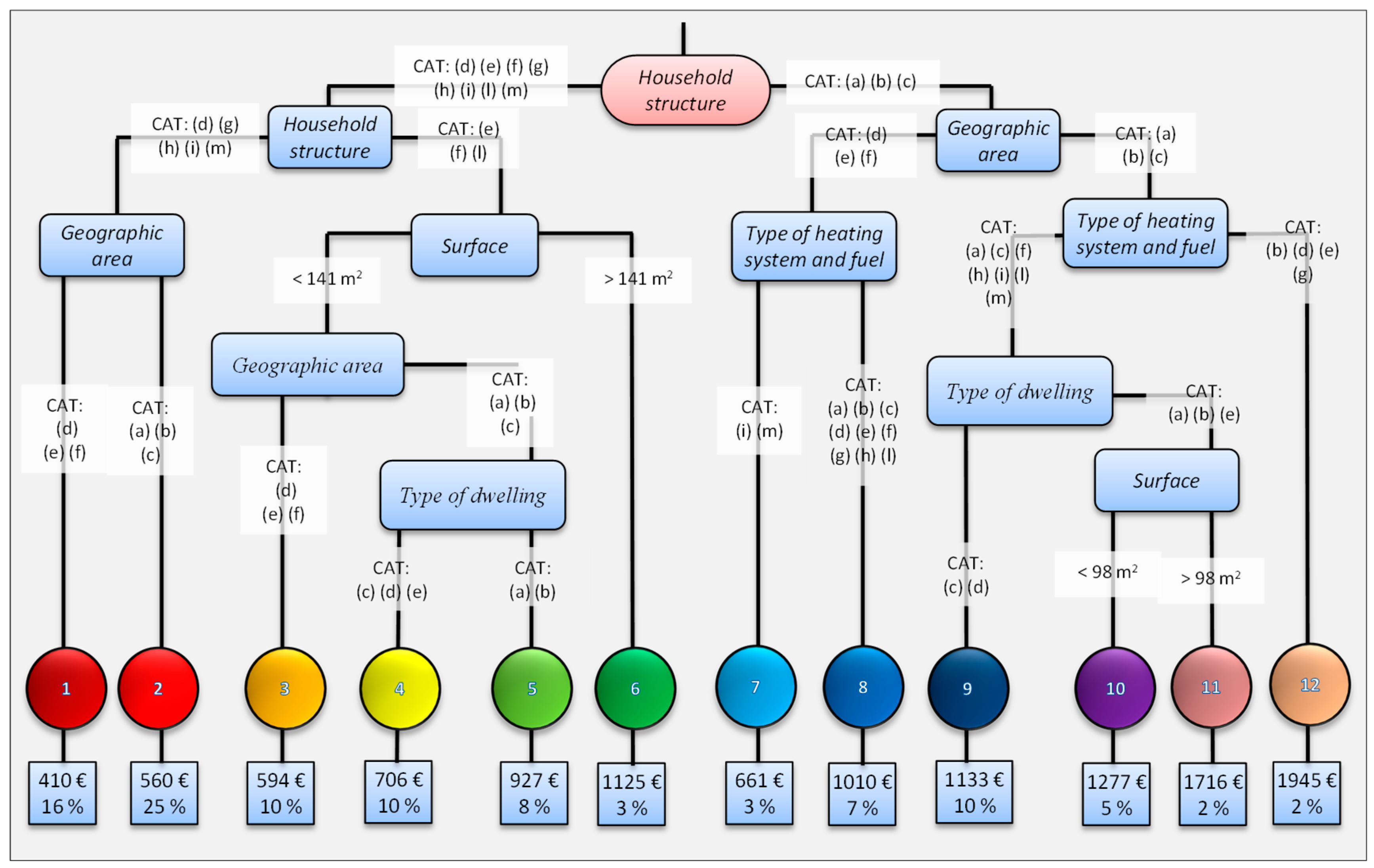
2.1. Dataset and Household Segmentation

The “Household Budget Survey: microdata for research purposes” (reference year: 2015, [23]) is applied in this research. This dataset was obtained by the Italian National Institute of Statistics (ISTAT) and is representative of the whole Italian population. The data were collected from 15,015 households, in 502 different municipalities; for each household, more than 1264 variables are available concerning socio-demographic information, dwelling characteristics, appliances, and monthly expenditures. In our previous studies [24,25], different statistical methods have been used to determine the relationship between the energy expenditure and the household variables. In particular, it was found that building variables are significant determinants in defining the thermal energy expenditures/consumptions; on the other hand, socio-economic variables are significant determinants with respect to the electrical energy expenditures. Subsequently, a segmentation of the Italian families has been obtained to study the energy consumption patterns in Italy, by using a segmentation-tree approach (see the outcomes of [24]).
In this paper, the outcome of household segmentation (concerning the total per-capital annual energy expenditure) obtained by Besagni and Borgarello [24] is applied. Household segmentation summarizes the combination of the prevailing factors influencing energy expenditure patterns. This information is of particular interest, as it may show additional details when compared with regression methods and summarize the energy consumption patterns within Italian households. This household segmentation is displayed in Figure 1, and the classification is based on the following variables (listed in Table 1): Household structures (2 splits), geographic area (3 splits), heating type and system (2 splits), floor surface (2 splits), and dwelling type (2 splits). In Figure 1, it can be observed that the first, and most important, splitting is based on the household structure and the splitting divide between “single-person-based households” and “non-single-person-based households”; subsequently, the geographical dimension and the dwelling characteristics are used. It is worth noting that, in the segmentation tree, socio-demographic and building variables have been used; conversely, no appliance variables have been applied; this result suggests that, despite the fact that appliance variables are important in determining higher energy expenditures when comparing different households, they cannot be used to select homogeneous groups of households. Further details regarding statistical methods, thresholds, and interpretation of the results were provided in [24,25], which the reader may refer to.

2.2. Measures of Fuel Poverty

In order to contribute to the existing discussion on suitable indicators to quantify the incidence of fuel poverty at the “country scale” in Italy, eight indicators have been applied to the data available in the “Household Budget Survey: microdata for research purposes” and, subsequently, the outcomes of the results have been presented based on the household segmentation (see Figure 1). In particular, seven indicators taken from the literature (#1–#7, in the following) have been applied and a novel indicator (#8, in the following), based on the minimum thermal comfort constraint, has been further developed:
  • Criterion #1. Energy expenditure is lower than half of the median [26];
  • Criterion #2. Incidence of energy expenditure on the total household expenditure is higher than double of the median [26];
  • Criterion #3. Condition of absolute poverty: This criterion has been used as, in the dataset, no information concerning the income of the households is available to apply income-based criteria;
  • Criterion #4. Energy expenditure is higher than double of the median [27];
  • Criterion #5. Energy expenditure is higher, compared with food expenditure [27];
  • Criterion #6. Household having scarce economic resources—this criterion has been used as, in the dataset, no information concerning the income of the households is available to apply income-based criteria;
  • Criterion #7. Household having insufficient economic resources—this criterion has been used as, in the dataset, no information concerning the income of the households is available to apply income-based criteria; and
  • Criterion #8. Households having thermal energy expenditure below the limit to reach a minimum comfort condition [21]. This indicator considers the thermal energy expenditure for heating purposes. The inclusion of the cooling load within fuel poverty definition has not been considered so far, to our knowledge, but would be a promising step forward with the respect to the present body of knowledge and an interesting point of view for future studies.

2.3. “Minimum Thermal Comfort Constraint” Criterion: Details and Implementation

As discussed in the introduction, the “minimum thermal comfort” criterion is supposed to overcome some of the limitations of the existing indicators (namely, the “10% indicator”, the “minimum income standard indicator”, and the “low income/high cost indicator”), as it considers the demand side by detailed lumped parameter modeling (which was a shortcoming in the low income/high cost indicator). The main advantage of the “minimum thermal comfort” measure is that it does not need to assess the condition of energy vulnerability based on a priori thresholds, but is defined according to the specific properties of each dwelling (i.e., period of construction of the dwelling, region of residence, number of members of the family, and so on). In particular, the “minimum thermal comfort” criterion was developed by integrating different modeling approaches in a four-step procedure. First, a lumped parameter model is applied to compute the annual “baseline thermal energy requirement” for the different household types. Second, the “baseline thermal energy requirements” are converted into the “minimal thermal energy requirements (based on comfort constraints)”. Third, the “minimal thermal energy requirements” are converted into “minimal thermal energy expenditures”. Finally, the data provided in the “Household Budget Survey: microdata for research” are post-processed to compute the annual “real thermal energy expenditures”. At this point, the annual “real thermal energy expenditures” are compared with the “minimal thermal energy expenditures”, to evaluate fuel-poor households.

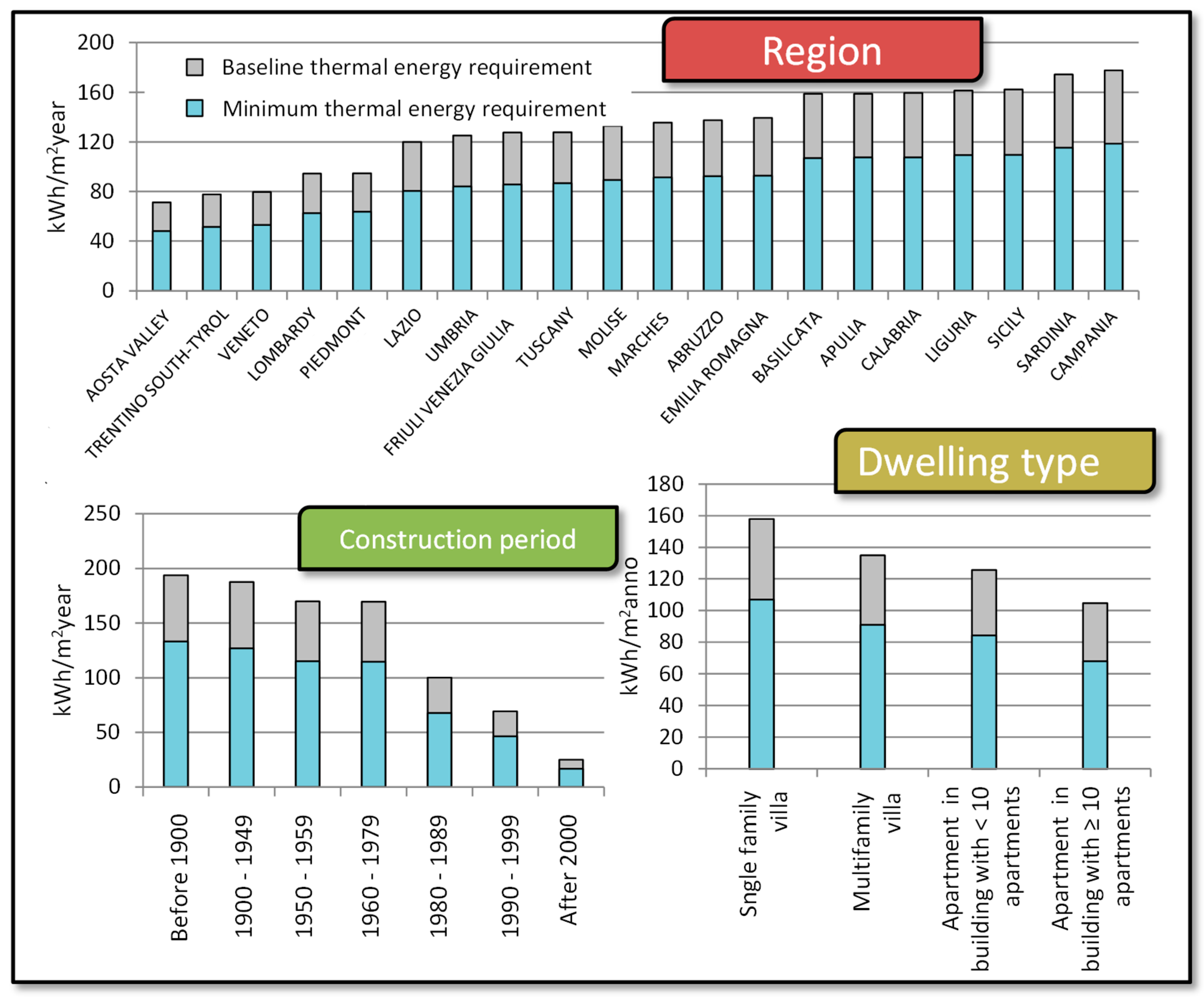
2.3.1. Baseline Thermal Energy Requirement

The lumped parameter model described in UNI-EN-ISO 13790:2008 [28] allows computing of the annual heating requirements (FBaseline). Capozza et al. [29] and Ballarini et al. [30] applied this method to obtain the annual baseline household heating requirements (FBaseline,Capozza—see Table 15 in [29]) for 140 residential buildings representative of the Italian building stock, classified in terms of dwelling type, construction period, and climatic zone, and defined as follows:
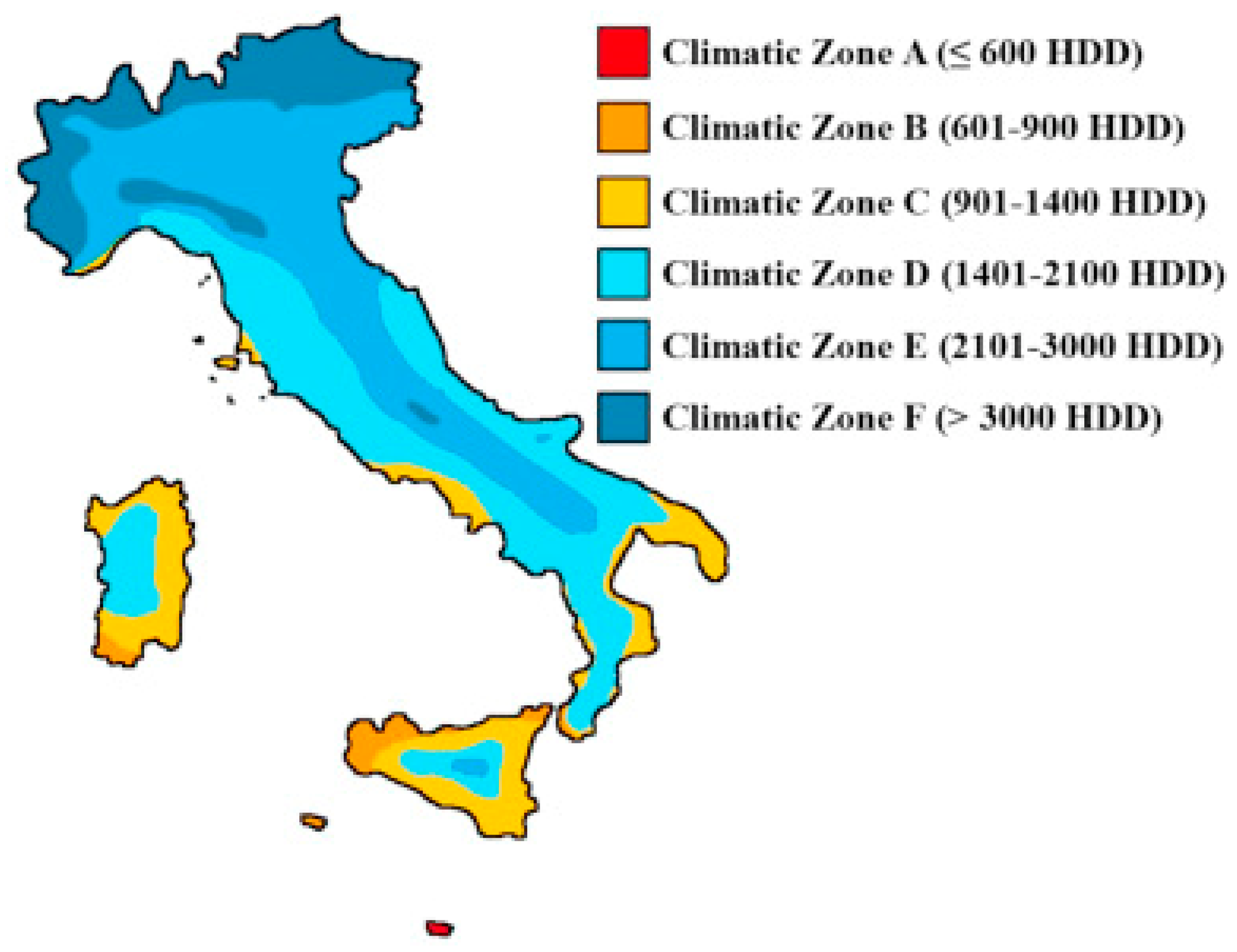
  • Climatic zone, classified based on the heating degree days (HDD), as reported in the Italian regulation [17] (Figure 3): (a) Zone “B” (600 < HDD ≤ 900); (b) zone “C” (900 < HDD ≤ 1400); (c) zone “D” (1400 < HDD ≤ 2100); (d) zone “E” (2100 < HDD ≤ 3000); and (e) zone “F” (HDD > 3000). Zone “A” (≤ 600 HDD) was not considered, as it is not representative [25]. The heating period, for the different climatic zones, and the number of hours when the heating system was turned on, are selected based on the current regulations in Italy [31].
  • Dwelling type: (a) Single-family house (B1); (b) terraced house (B2); (c) multi-family house (B3); and (d) apartment block (B4).
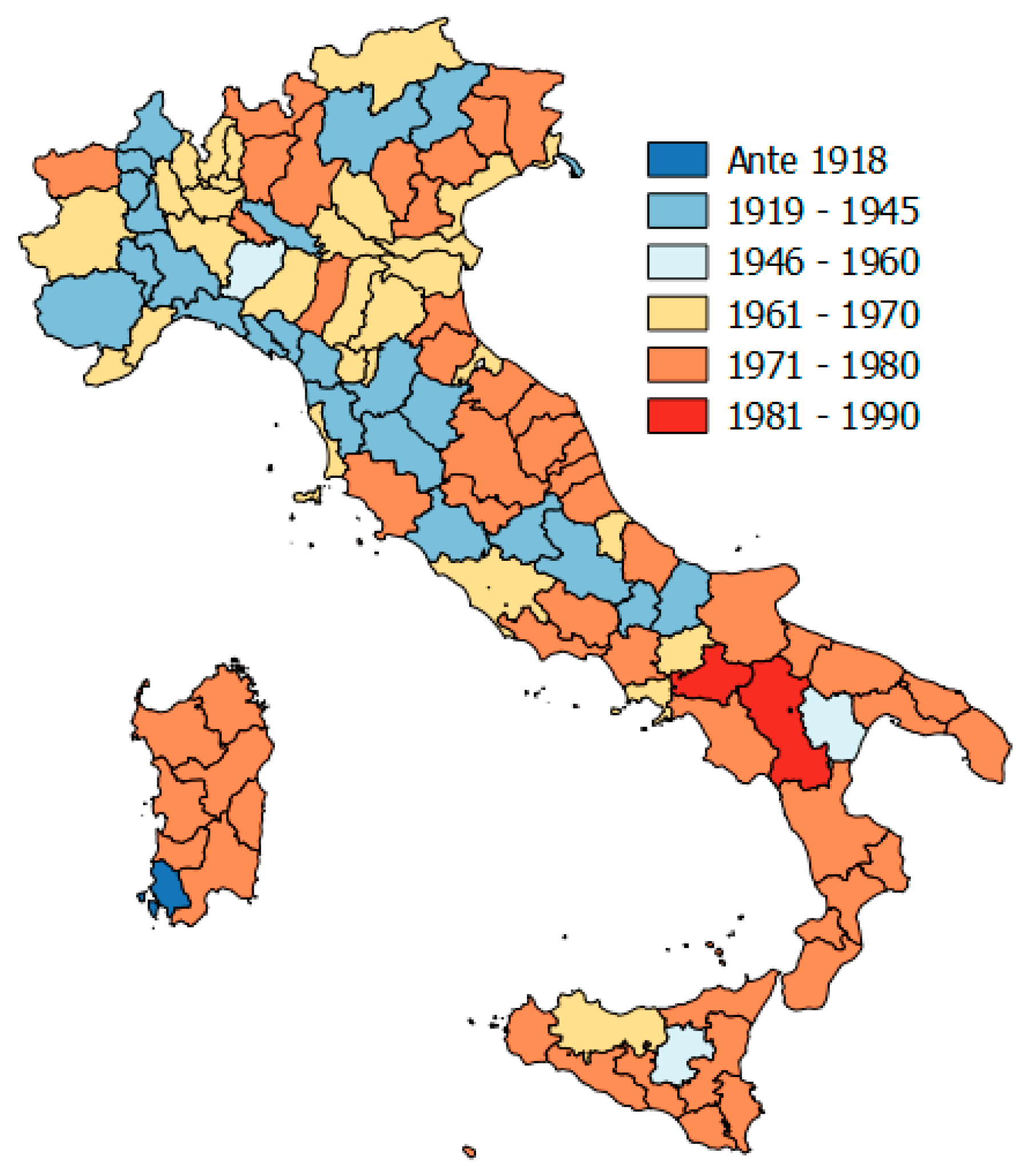
  • Construction period (see Figure 4): (a) Ante-1920 (V1), (b) 1921–1945 (V2), (c) 1946–1960 (V3), (d) 1961–1975 (V4), (e) 1976–1990 (V5), (f) 1991–2005 (V6), and (g) 2005–ongoing (V7);
The above-mentioned 140 dwelling types are characterized by different thermophysical properties (i.e., thermal transmission coefficients of the glazed and opaque components, geometrical details, and so on); these input data are listed in [32]. The meteorological data, for the different zones, have been implemented, based on the data in [33].
The annual baseline household heating requirements computed by Capozza et al. [29] refer to 2006; conversely, the “Household Budget Survey” considers the 2015 situation. For this reason, a calibration procedure is needed and Faiella et al. [21] suggested a calibration, based on the overall Italian energy consumption ( C 2006 = 29.54   Mtep and C 2015 = 23.73   Mtep ). The household heating requirements computed by Capozza et al. [29] are corrected, as in Equation (1):
F Baseline , Capozza , 2015 = F Baseline , Capozza   C 2015 C 2006 .
It is worth noting that the data used by Capozza et al. [29] cannot be coupled, as they are, with the “Household Budget Survey” dataset (see the tables provided by Besagni and Borgarello [24]): In order to assign a heating requirement to every household in the dataset, the variables selected by Capozza et al. [29] and the variables in the “Household Budget Survey” dataset need to be matched. To this end, the following criteria have been applied, following Besagni and Borgarello [25]:
  • Geographic region: The geographic locations employed by Capozza et al. [29] concern the above-mentioned climatic zones; conversely, in the dataset, different Italian regions were used. As the climatic zones are based on HDDs, the annual baseline household heating requirement for the different regions ( F Baseline , 2015 , region k ), were computed by a weighted average, based on the extension of the climatic bands inside the different regions. The extension of the climatic areas is approximated by counting the number of municipalities (nm), in each region, corresponding to the different climatic zones:
    F Baseline , 2015 , region k = j = 1 5 F Baseline , Capozza , 2015 , j · nm k , j j = 1 5 nm k , j ,
    where j is the j-climatic area and k is the k-region.
  • Construction period: V1 is matched with “Before 1900”; V2 is matched with “Between 1900 and 1949”; V3 is matched with “Between 1950 and 1959”; V4 is matched with “Between 1960 and 1969” and “Between 1970 and 1979”; V5 is matched with “Between 1980 and 1989”; V6 is matched with “Between 1990 and 1999”; and V7 is matched with “Between 2000 and 2009” and “After 2009”.
  • Dwelling type: B1 is matched with “Single family villa”; B2 is matched with “Multifamily villa”; B3 is matched with “Apartments in building with less than 10 apartments” and “other”; and B4 is matched with “Apartments in building with 10 or more apartments”.

2.3.2. Minimum Thermal Energy Requirement

In the previous section, the baseline thermal energy requirements were computed. These data need to be converted into minimum thermal energy requirements, based on which two corrections are applied. The first correction, related to the crowding effect, is applied. Hence, to account for the influence of the number of occupants and the size of the building on energy consumption for heating purposes, the correction defined in Equation (3) should be applied (based on [24]):
F Baseline , 2015 , region k , IA = F Baseline , 2015 , region k [ 1 + α ( IA eff - IA std IA std ) ] ,
where α = -0.06 and the heat requirement corrected for the crowding effect (the left side of Equation (3)), may either increase or decrease as a function of IAeff (related to the household variables) and IAstd (constant value). These parameters depend on the number of occupants (Noccupants) and the surface of the dwelling (Adwelling), as follows:
IA eff = N occupants A dwelling ,
IA std = N occupants , standard - value A dwelling , standard - value = 1 40 .
The second correction is related to the comfort conditions (CC) inside the household: The expected levels of comfort are defined based on the European standard EN 15251 [34] and are divided into three categories, based on operating temperatures (TOp,eff) [35]:
  • CC1: High comfort conditions → T Op , Eff = 20.5 ° C ;
  • CC2: Normal comfort conditions → T Op , Eff = 18.6 ° C ; and
  • CC3: Low comfort conditions → T Op , Eff = 17.5 ° C .
As with Faiella et al. [21], the conditions CC3 were selected. Thus, the left side of Equation (3) is corrected by Equation (6):
F Baseline , 2015 , region k , MIN = F Baseline , 2015 , region k , IA [ 1 + γ ( T Op , Eff T Op , STD ) ] ,
where TOp,eff is the standard operating temperature, equal to 20 °C, while γ = 0.13 [1/°C]. This procedure was applied to all the households in the dataset. As an outcome, Figure 5 displays the comparison between the baseline thermal energy requirement and the minimum thermal energy requirement. In particular, Figure 5 presents the results in terms of construction period, dwelling type, and geographic region. Finally, the minimum heating requirements per unit area can be assigned to the different households in the dataset, by multiplying their value for the corresponding floor area:
F Baseline , 2015 , region k , MIN , S = F Baseline , 2015 , region k , MIN × A dwelling .

2.3.3. Minimum Thermal Energy Expenditure

In the “Household Budget Survey” dataset, expenditure data are available; thus, the heating requirements should be converted into corresponding expenditures. To this end, the data obtained in Equation (8) have been converted into equivalent standard cubic meters of natural gas (NG), as follows:
NG = F Baseline , 2015 , region k , MIN , S ω GN ,
where ω GN = 0.914 [ Sm 3 / kWh ] (reference technology: convectional boiler); from a theoretical point of view, ω GN depends on the type of energy conversion system, the altitude of the municipality, the climate zone, and the number of heating system operation days. Finally, the equivalent standard cubic meters of natural gas are converted into thermal expenditure (SComfort,MIN,i) by considering the cost of natural gas in the reference year 2015 [36]. In this procedure, the costs for Sardinia were supposed equal to the ones for Sicily. The hypothesis underlying Equation (8) is that the heat requirement is completely satisfied by using natural gas; this assumption is supported by the fact that, in Italy, the main source of energy for the heating of the home and water is gas, used by >70% of all households. Future studies could improve this estimate by considering the different sources of thermal energy.

2.3.4. Real Thermal Energy Expenditure

In the “Household Budget Survey” dataset, expenditures were provided in terms of monthly data and considered the following components: (a) Gas from a network, (b) central heating, (c) district heating, (d) liquid gases, (e) liquid fuels, (f) coal, and (g) solid fuels. As stated above, in Italy, the main source of energy for heating purposes and domestic hot water is gas and, thus, the comparison with the outcome of Equation (8) can be considered acceptable, at least as a first approximation. It is known that the demand side determining the heating/cooling loads in buildings consists of the household side and an ambient side. The former is intrinsically present in the statistical dataset; conversely, the latter has been discussed by Besagni and Boregarello [24]. In particular, in [24], a method to convert the monthly energy expenditures into annual energy expenditures has been proposed (see Appendix A of [24]); the same procedure was applied in this paper to obtain the SReal,i data.

3. Results

The fuel poverty indicators, presented in Section 2.2 and Section 2.3, were applied to the household segmentation presented in Figure 1. The results of this analysis are displayed in Table 2 and Figure 6 and Figure 7. Table 2 displays the percentage of families satisfying the different conditions within each cluster and provides an overview regrading vulnerability in the Italian households. Figure 6 displays the distribution of vulnerable households, according to the different criteria inside each cluster. Finally, Figure 7 displays the percentage of households, within each cluster, satisfying a certain number of indicators. According to the data in Table 2, the following syntactic outcomes can be drawn for the different criteria:
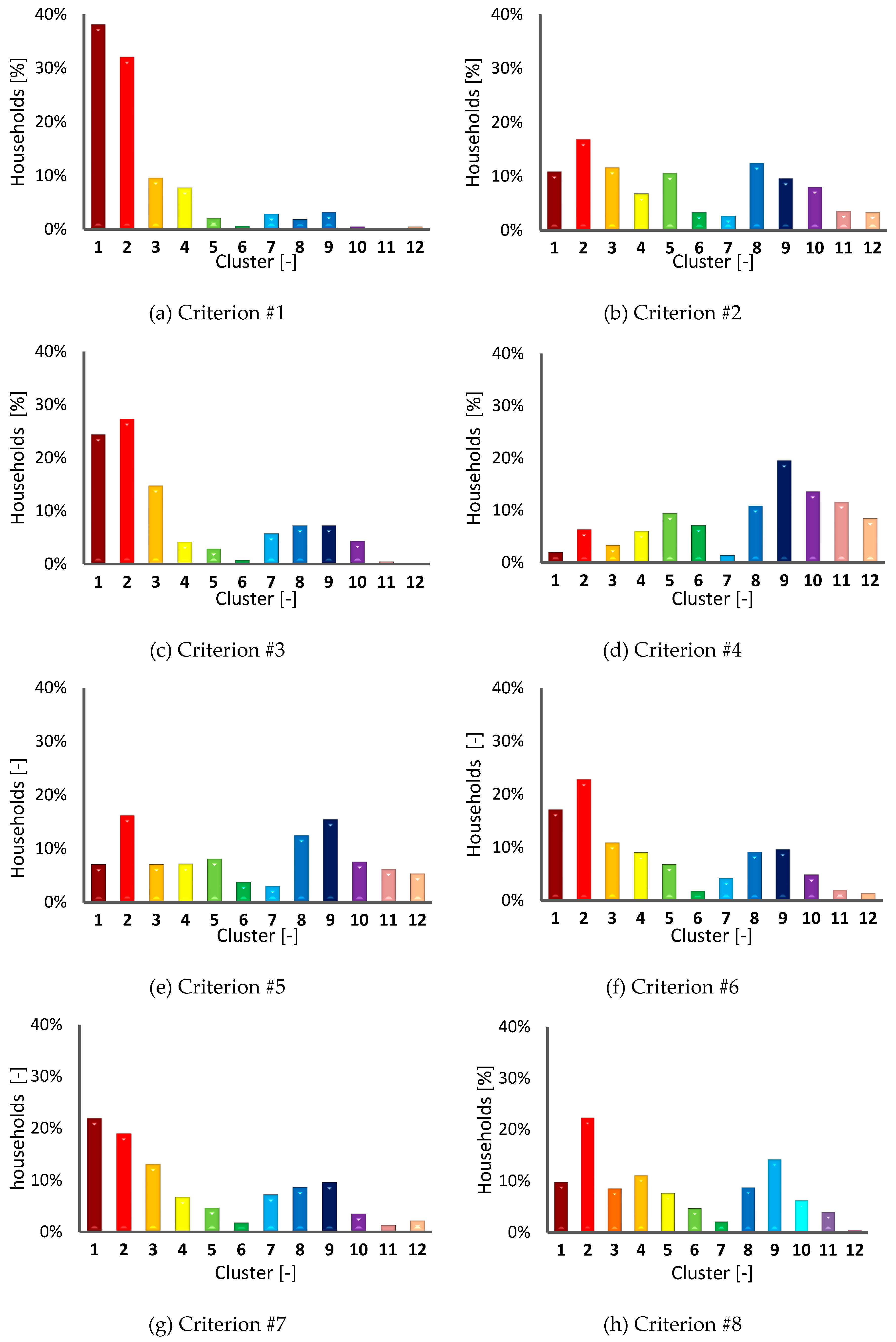
  • Criterion #1. Cluster #1 (39.7%), cluster #2 (21.2%), cluster #3 (16.2%), and cluster #7 (16.2%) contain a high percentage of households satisfying this criterion;
  • Criterion #2. Cluster #12 (31.9%), cluster #10 (25.2%), cluster #8 (24.2%), and cluster #11 (22.1%) contain a high percentage of households satisfying this criterion;
  • Criterion #3. Cluster #7 (10.1%), cluster #1 (8.2%) and cluster #3 (8.0%) contain a high percentage of household satisfying this criterion;
  • Criterion #4. Cluster #12 (50.9%) and cluster #11 (45.1%) contain a high percentage of households satisfying this criterion;
  • Criterion #5. Cluster #12 (22.6%), cluster #11 (17.0%), cluster #8 (10.7%) and cluster #10 (10.6%) contain a high percentage of households satisfying this criterion;
  • Criterion #6. Cluster #7 (53.0%), cluster #8 (46.5%), cluster #3 (42.0%) and cluster #1 (40.9%) contain a high percentage of households satisfying this criterion;
  • Criterion #7. Cluster #7 (18.2%), cluster #12 (11.1%), cluster #1 (10.6%) and cluster #3 (10.2%) contain a high percentage of households satisfying this criterion; and
  • Criterion #8. Cluster #7 (44.7%), cluster #11 (11.1%) and cluster #6 (43.0%) and cluster#3 (41.5%) contain a high percentage of households satisfying this criterion.
Considering the data in Figure 2, some insights into the results can be drawn, based on two perspectives: (a) Looking at the most vulnerable clusters for a given criterion and (b) looking at the most critical criterion for a given cluster.
Concerning the most vulnerable clusters for a given criterion, the main results are as follows: The indicator that evaluates whether energy expenditure is less than half the median suggested an higher incidence of fuel poverty within cluster #1; conversely, the indicators regarding the incidence of energy expenditure on the other expenditures suggested an higher risk of fuel poverty in cluster #12 (namely, the incidence of energy expenditure on total expenditure, energy expenditure above twice the average, and energy expenditure higher than food expenditure). On the other hand, the remaining indicators suggested a higher incidence of fuel poverty within cluster #7 (i.e., absolute poverty, scarce economic resources, insufficient economic resources, and comfort-based indicators).
Concerning the most critical criteria for a given cluster, the main results are as follows: In cluster #1, the greatest vulnerability factor was related to the economic variables; in cluster #2, cluster #5, and cluster #9, the greatest vulnerability factor was related to the comfort-based criterion; cluster #3 was similar to cluster #1, but the possibility of not reaching heat requirements was slightly higher; in cluster #4, there was a larger share of households with insufficient economic resources; cluster #6 proved that it is difficult to achieve adequate thermal comfort, even when households exhibited high energy expenditure (see the data in Figure 1); in cluster #7, the highest levels of risk of fuel poverty were identified for two indicators: (a) Decrease in the economic resources criterion and (b) the thermal comfort criterion. It can be observed that the households in cluster #8 used an high share of their available income to achieve adequate energy comfort conditions, and the risk of not achieving comfort conditions was relevant; cluster #9 was among the clusters with a lower level of vulnerability; also, in cluster #10, a non-negligible vulnerability was observed with respect to the comfort-based criterion; cluster #11 exhibited a relevant incidence of high energy expenditures, with respect to the total expenditures; cluster#12 was associated with a relevant incidence of fuel poverty incidence, when considering different indicators.
Further insights in above-discussed results can be provided by looking at the data in Figure 6. The households with annual per-capita energy expenditures lower than half of the median were mostly located within cluster #1 and cluster #2; households with high incidence of energy expenditure on the total expenditure were mainly located within cluster #2, and, subsequently, within cluster #1, cluster #3, cluster #5, and cluster #8; with respect to the absolute poverty indicator, higher incidence is observed within cluster #1, cluster #2, and cluster #3. The higher share of household with energy expenditure above twice the median was within inside cluster #9; households spending more for energy rather than food were mainly located within cluster #2, cluster #9, and cluster #8; the distributions of households with scarce and insufficient economic resources were similar, and were mainly located within cluster #1 and cluster #2. The thermal comfort indicator outlined a more critical situation within cluster #2. A further insight may be proposed by observing the whole set of indicators. To this end, Figure 7 provides a graphical representation of the percentage of families, within each cluster, that satisfy at least two, three, or four criteria. In this respect, cluster #11, cluster #12, and cluster #10 were the ones with higher incidences of fuel poverty issues, as they had a higher share of households satisfying at least three indicators at the same time. When we increased the constraints to four indicators satisfied at the same time, the most vulnerable clusters were cluster #12, cluster #8, and, subsequently, clusters #10 and #11. Generally speaking, the proposed analysis shows that there were some groups of households where the level of vulnerability, with respect to fuel poverty, was quite low (i.e., cluster #4); conversely, other groups had a high risk of fuel poverty issues (cluster #12 and cluster #7).

4. Conclusions

Using a nationally-representative sample of Italian households (reference year: 2015), this paper contributes to the existing discussion on fuel poverty in Italy. The proposed case study is particularly interesting, as the Italian country is peculiar in terms of climatic conditions, dwelling types, and its many socio-demographic dimensions. To this end, different indicators have been applied to a national household segmentation: Both indicators taken from the literature, as well as a novel indicator based on the “minimum thermal comfort” constraint, have been applied. The proposed analysis shows that there are some groups where the level of vulnerability, with respect to fuel poverty, is quite low (i.e., cluster #4 in Figure 1), and others in which the risk is high (i.e., clusters #12 and #7 in Figure 1). It is worth noting that this analysis is a preliminary assessment and future studies should be applied by using additional datasets, especially those including income data. From a practical point of view, this study suggests that there is a section of the Italian households more vulnerable, with respect to fuel poverty issues, compared to the other sections. This outcome is of fundamental importance to assist policy-makers in developing incentives to tackle fuel poverty issues at the household level. From a practical point of view, this paper provides guidelines regarding the household types which incentives to tackle fuel poverty issues should give higher priority. It is worth noting that the proposed study suffers from some limitations that should be further addressed in the future: (i) That natural gas energy sources are only used in the computational procedure; (ii) the lack of data regarding precise income values; (iii) the employed dataset covers only one reference year; and (iv) the use of energy for cooling purposes is not considered. All these limitations may be tackled, in forthcoming activities, by coupling the employed dataset with additional ones.

Author Contributions

The contribution of the authors is described in the followings. Conceptualization, M.B. and G.B.; methodology, M.B. and G.B.; formal analysis, G.B.; investigation, G.B.; writing—original draft preparation, G.B.; writing—review and editing, M.B. and G.B.

Funding

This work has been financed by the Research Fund for the Italian Electrical System, in compliance with the Decree of Minister of Economic Development April 16, 2018.

Conflicts of Interest

The authors declare no conflict of interest.

References

  1. Isherwood, R.M.; Hancock, B.C. Household Expenditure On fuel: Distributional Aspects; Economic Adviser’s OfficeDHSS: London, UK, 1979. [Google Scholar]
  2. Boardman, B. Fuel poverty: From Cold Homes to Affordable Warmth; Pinter Pub. Limited: London, UK, 1991. [Google Scholar]
  3. Li, K.; Lloyd, B.; Liang, X.J.; Wei, Y.M. Energy poor or fuel poor: What are the differences? Energy Policy 2014, 68, 476–481. [Google Scholar] [CrossRef]
  4. Liddell, C.M. Fuel poverty comes of age: Commemorating 21 years of research and policy. Energy Policy 2012, 49, 2–5. [Google Scholar] [CrossRef]
  5. Herrero, S.T. Energy poverty indicators: A critical review of methods. Indoor Built Environ. 2017, 26, 1018–1031. [Google Scholar] [CrossRef]
  6. Karásek, J.; Pojar, J. Programme to reduce energy poverty in the Czech Republic. Energy Policy 2018, 115, 131–137. [Google Scholar] [CrossRef]
  7. Castaño-Rosa, R.; Solís-Guzmán, J.; Rubio-Bellido, C.; Marrero, M. Towards a multiple-indicator approach to Energy Poverty in the European Union: A review. Energy Build. 2019, 193, 36–48. [Google Scholar] [CrossRef]
  8. European Observatory on Energy Poverty (EPOV). Available online: www.energypoverty.eu (accessed on 1 April 2019).
  9. Heindl, P. Measuring fuel poverty: General considerations and application to German household data. FinanzArchiv Public Financ. Anal. 2015, 71, 178–215. [Google Scholar] [CrossRef]
  10. Hills, J. Fuel Poverty: The Problem and Its Measurement—Interim Report of the Fuel Poverty Review; CASE Report; Deparment for Energy and Climate Change: London, UK, 2011.
  11. Moore, R. Definitions of fuel poverty: Implications for policy. Energy Policy 2012, 49, 19–26. [Google Scholar] [CrossRef]
  12. Bradshaw, J.; Middleton, S.; Davis, A.; Oldfield, N.; Smith, N.; Cusworth, L.; Williams, J. A Minimum Income Standard for Britain: What people Think; Joseph Rowntree Foundation: York, UK, 2008. [Google Scholar]
  13. Hills, J. Fuel Getting the Measure of Fuel Poverty. Final Report of the Fuel Poverty Review; CASE Report; Centre for the Analysis of Social Exclusion: London, UK, 2012. [Google Scholar]
  14. Preston, I.; White, V.; Blacklaws, K.; Hirsh, D. Fuel Poverty: Fuel and Poverty: A Rapid Evidence; CASE Report; Assessment for the Joseph Rowntree Foundation Centre for Sustainable Energy: Bristol, UK, 2014. [Google Scholar]
  15. Middlemiss, L. A critical analysis of the new politics of fuel poverty in England. Crit. Soc. Policy 2017, 37, 425–443. [Google Scholar] [CrossRef]
  16. Rademaekers, K.; Yearwood, J.; Ferreira, A.; Pye, S.; Ian Hamilton, P.; Agnolucci, D.G.; Karásek, J.; Anisimova, N. Selecting Indicators to Measure Energy Poverty Rotterdam; Framework Contract ENER/A4/516-2014; Trinomics: Rotterdam, The Netherlands, 2016. [Google Scholar]
  17. Romero, J.C.; Linares, P.; López Otero, X.; Labandeira, X.; Pérez Alonso, A. Energy Poverty in Spain, Economic Analysis and Proposals for Action; Economics for Energy: Madrid, Spain, 2015. [Google Scholar]
  18. Zhao, Q.R.; Chen, Q.H.; Xiao, Y.T.; Tian, G.Q.; Chu, X.L.; Liu, Q.M. Saving forests through development? Fuelwood consumption and the energy-ladder hypothesis in rural Southern China. Transform. Bus. Econ. 2017, 16, 199–219. [Google Scholar]
  19. Baležentis, T.; Štreimikienė, D.; Melnikienė, R.; Zeng, S.Z. Prospects of green growth in the electricity sector in Baltic States: Pinch analysis based on ecological footprint. Resour. Conserv. Recycl. 2019, 142, 37–48. [Google Scholar] [CrossRef]
  20. Zeng, S.Z.; Baležentis, T.; Streimikiene, D. Review of and Comparative Assessment of Energy Security in Baltic States. Renew. Sustain. Energy Rev. 2017, 76, 185–192. [Google Scholar] [CrossRef]
  21. Faiella, I.; Lavecchia, L.; Borgarello, M. Una Nuova Misura Della Povertà Energetica Delle Famiglie (A New Measure of Households’ Energy Poverty). Questioni di Economica e Finanza (Occasional Papers) 2017, 404, 1–16. [Google Scholar]
  22. Romero, J.C.; Linares, P.; López, X. The policy implications of energy poverty indicators. Energy Policy 2018, 115, 98–108. [Google Scholar] [CrossRef]
  23. Italian National Institute of Statistics (ISTAT). Household Budget Survey: Microdata for Research Purposes (Reference Year: 2015); ISTAT: Rome, Italy, 2017. [Google Scholar]
  24. Besagni, G.; Borgarello, M. The determinants of residential energy expenditure in Italy. Energy 2019, 165, 369–386. [Google Scholar] [CrossRef]
  25. Besagni, G.; Borgarello, M. The socio-demographic and geographical dimensions of fuel poverty in Italy. Energy Res. Soc. Sci. 2019, 49, 192–203. [Google Scholar] [CrossRef]
  26. EUROSTAT, 2010 Household Budget Survey. Available online: https://ec.europa.eu/eurostat/web/microdata/household-budget-survey (accessed on 1 April 2019).
  27. Ürge-Vorsatz, D.; Herrero, S.T. Building synergies between climate change mitigation and energy poverty alleviation. Energy Policy 2012, 49, 83–90. [Google Scholar] [CrossRef]
  28. UNI EN ISO 13790:2008. Prestazione energetica degli edifici—Calcolo del fabbisogno di energia per il riscaldamento e il raffrescamento. 2008. [Google Scholar]
  29. Capozza, A.; Carrara, F.; Gobbi, E.; Madonna, F.; Ravasio, F.; Panzeri, A. Analisi tecnico-economica di interventi di riqualificazione energetica del parco edilizio residenziale Italiano; RdS Report 14002104; RdS: Milan, Italy, 2013. [Google Scholar]
  30. Ballarini, I.; Corrado, V.; Madonna, F.; Paduos, S.; Ravasio, F. Energy refurbishment of the Italian residential building stock: Energy and cost analysis through the application of the building typology. Energy Policy 2017, 105, 148–160. [Google Scholar] [CrossRef]
  31. D.P.R. 16 aprile 2013, n 74. 2013. Regolamento recante norme per la progettazione, l’installazione, l’esercizio e la manutenzione degli impianti termici degli edifici ai fini del contenimento dei consumi di energia, in attuazione dell’art. 4, comma 4, della legge 9 gennaio 1991, Gazzetta Ufficiale della Repubblica Italiana. Available online: www.gazzettaufficiale.it/eli/id/2013/06/27/13G00114/sg (accessed on 1 April 2019).
  32. Madonna, F.; Corrado, V. Studio sulla riqualificazione energetica di edifici residenziali; RdS Report 14002701; RdS: Milan, Italy, 2014. [Google Scholar]
  33. Mazzarella, L. Dati climatici G. de Giorgio. In Proceedings of the Giornata di Studio Giovanni De Giorgio; Politecnico di Milano: Milan, Italy, 1997. [Google Scholar]
  34. Comité Européen de Normalisation. CEN Standard EN15251—Indoor Environmental Input Parameters for Design and Assessment of Energy Performance of Buildings—Addressing Indoor Air Quality, Thermal Environment, Lighting and Acoustics; Comité Européen de Normalisation: Brussels, Belgium, 2007. [Google Scholar]
  35. Madonna, F.; Quaglia, P. Riqualificazioni energetiche: Benefici di comfort e costi; Internal Report; Ricerca sul Sistema Energetico - RSE S.p.A.: Milan, Italy, 2016. [Google Scholar]
  36. Autorità di Regolazione per Energia Reti e Ambiente (ARERA). Available online: www.arera.it (accessed on 1 April 2019).
Figure 1. Household segmentation (total per-capital annual energy expenditure) obtained by Besagni and Borgarello [24]. Code names of the splits are listed in Table 1.
Sustainability 11 02732 g001
Figure 2. Descriptive analysis of the floor area.
Sustainability 11 02732 g002
Figure 3. Climatic regions in Italy [30].
Sustainability 11 02732 g003
Figure 4. Period of construction of buildings in Italy.
Sustainability 11 02732 g004
Figure 5. Baseline and the minimum thermal energy requirements. The details for obtaining these data are provided in Section 2.3.1 and Section 2.3.2.
Sustainability 11 02732 g005
Figure 6. Applications of fuel poverty criteria to the household segmentation: Distribution of households that meet a certain criterion within each cluster (Refer to Figure 1 for the cluster classification within the national household segmentation).
Sustainability 11 02732 g006
Figure 7. Percentage of households satisfying a certain number of indicators in each cluster.
Sustainability 11 02732 g007
Table 1. Code names of the variables in Figure 1 with their summary statistics. * HRP = Household Representative Person. ** Summary statistics evaluated on the whole data-set. *** See Figure 2 for a detailed descriptive analysis.
VariableSummary Statistics ** and Code Names for Figure 1
Household structure *(a) Single person 18–34 years (391), (b) Single person 35–64 years (1817), (c) Single person 65 years and more (2240), (d) Couple without children with HRP 18–34 years (178), (e) Couple without children with HRP 35-64 years (1350), (f) Couple without children with HRP 65 years and more (2164), (g) Couple with 1 child (2276), (h) Couple with 2 children (2184), (i) Couple with 3 children or more (495), (l) Mono parent family (1033), (m) Others (885)
Geographic location(a) North-west (3284), (b) North-east (3382), (c) Centre (2791), (d) South (4385), (e) Sicily (753), (f) Sardinia (418)
Type of dwelling(a) Single family villa (2738), (b) Multifamily villa (4587), (c) Apartments in building with less than 10 apartments (3733), (d) Apartments in building with 10 or more apartments (3939), (e) Other (16)
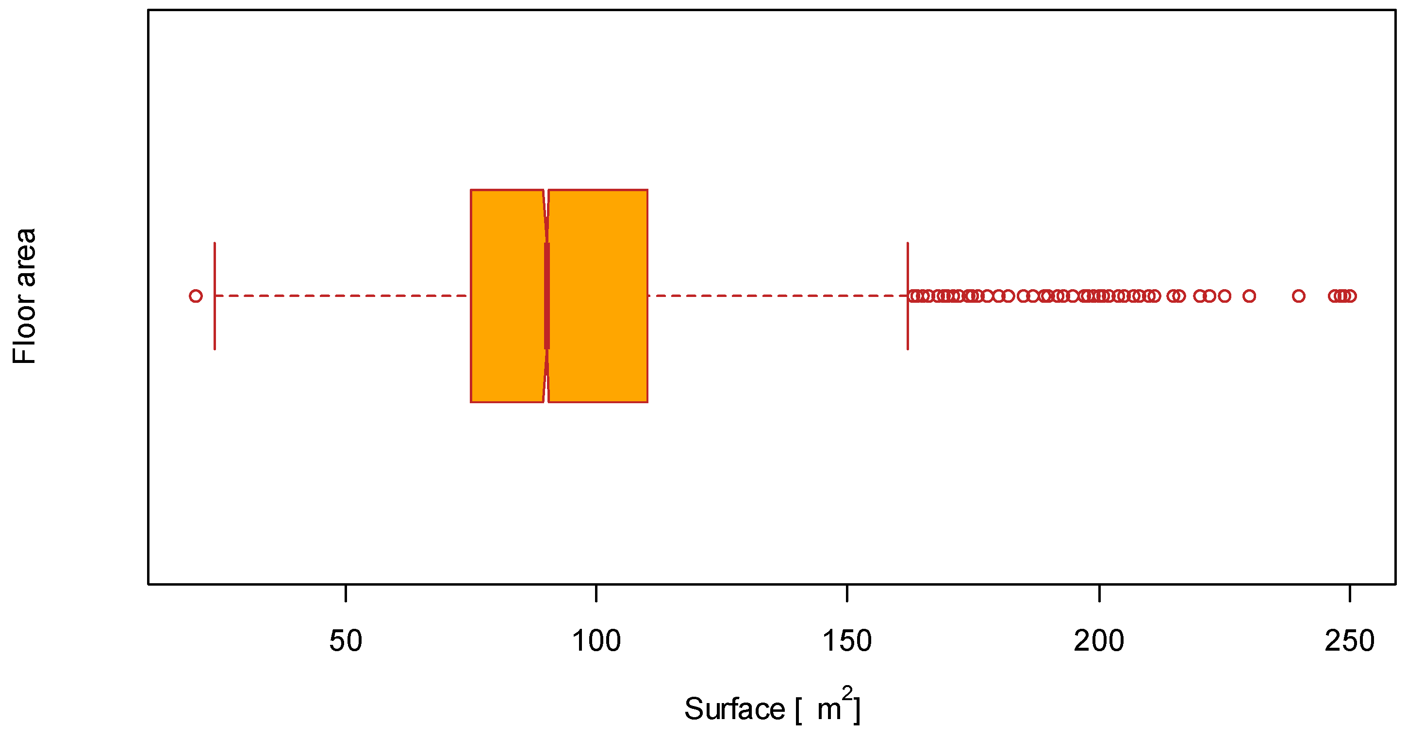
Floor area ***Continuous variable [Mean = 98/Variance = 1342]
Table 2. Percentage of families inside a cluster satisfying specific criteria. Values in percentage. Color bar as follows: Red, maximum; and green, minimum.
Cluster/Criterion .#1#2#3#4#5#6#7#8
139.710.08.21.22.940.910.619.0
221.29.85.82.34.234.75.823.0
316.217.28.03.14.642.010.227.2
413.210.12.35.74.735.25.327.3
54.519.42.011.06.632.64.526.2
63.415.21.320.47.621.54.241.5
716.213.010.14.36.553.018.244.7
84.224.25.213.410.746.58.834.2
95.413.93.917.99.936.57.333.2
102.125.25.027.010.639.75.933.8
112.022.11.145.117.033.04.343.0
125.831.90.950.922.634.511.120.8
Refer to Figure 1 for the cluster classification within the national household segmentation.

