Article

Deviation of Peak Hours for Urban Rail Transit Stations: A Case Study in Xi’an, China

Department of Traffic Engineering, Highway School, Chang’an University, Xi’an 710064, China
*
Author to whom correspondence should be addressed.
Sustainability 2019, 11(10), 2733; https://doi.org/10.3390/su11102733
Submission received: 21 March 2019 / Revised: 1 May 2019 / Accepted: 5 May 2019 / Published: 14 May 2019
(This article belongs to the Special Issue Sustainable Urban Land Use and Transportation)

Abstract

:
The inconsistencies of passenger flow volume between stations’ peak hours and cities’ peak hours have emerged as a phenomenon in various cities worldwide. Passenger flow forecasting at planning stages can only predict passenger flow volume in city peak hours and for the whole day. For some stations, the highest flow does not occur in the city peak hours, and station scale design is often too small. This study locates the formation mechanism of station peak in which the temporal distribution of the station is the superposition of different temporal distributions of the purpose determined by land-use attributes. Data from 63 stations in Xi’an, China, were then used to present an enlargement coefficient which can change the boarding and alighting volume in city peak hours to a station’s own peak hours. This was done by analyzing the inconsistencies of passenger flow volume between the station’s peak hours and the city’s peak hours. Morning peak deviation coefficient (PDC) and evening PDC were selected as datasets, and stations were classified accordingly. Statistics of land usage for every type of station showed that when the stations were surrounded by developed land, the relationship between the PDC and the commuter travel land proportion was to some extent orderly. More than 90.00% of stations with a proportion of commuter travel land that was more than 0.50 had PDCs under 1.10. All stations with a proportion of commuter travel land that was less than 0.50 had morning PDCs over 1.10. Finally, data from 52 stations in Chongqing, China were used to verify the findings, with the results in Chongqing predominantly corresponding to those in Xi’an.

1. Introduction

Urban rail transit has existed for over 150 years, with global large-scale construction of urban rail transit emerging in the 1970s. At present, over 150 cities in over 50 countries have subways, with a total length reaching beyond 10,000 km.
Due to the long service life of urban rail, it is necessary to build rail transit according to passenger flow forecast results to adapt the rail for future travel traffic. As urban rail transit develops, research into passenger flow forecasting also continues to expand. Researchers initially studied the four-stage method, and have gradually developed more advanced passenger flow forecasting methods [1,2] which include total control, and the distribution of passenger flow on the rail transit network [3,4]. Some scholars have investigated the difference between actual operation results and the passenger flow forecast by analyzing the problems in passenger flow forecasting [5,6,7], shortcomings of the traditional four-stage method, and introducing improvements [8,9,10,11,12]. Rail transit lines gradually extend into the suburbs as cities develop and expand. Due to the difference between the mode of travel in the suburbs and in urban areas, research on the forecast method of passenger flow in suburban rail transit has also emerged [13,14,15,16]. To satisfy the demand for refined operations, a number of scholars have studied short-term passenger flow forecasting [17,18,19], and abnormal passenger flow forecasting [20,21]. Station scale also directly affects passenger perception of the rail transit service level. When studying the passenger flow of a station, its location, the nature of the land, and connection with other modes of transportation have emerged as important influencing factors [22,23,24,25]. The application of passenger flow forecasting results for the calculation of rail transit station scale has also been investigated [26,27].
With the operation of urban rail transit, it has become apparent in many areas that station peak hours are not completely consistent with those of the city. This phenomenon is referred to as the deviation of peak hours for urban rail transit stations in this paper. Peak hour deviation has emerged in the Chinese cities of Xi’an and Chongqing, where statistics have been collected. The statistical results are presented in Table 1. The data for Xi’an spans from September 2017 to May 2018, and is provided by Xi’an Metro Co., Ltd. The data for Chongqing is in 4 May 2016 (Wednesday), and is provided by Chongqing Rail Transit Co., Ltd. The two cities all possess unique features. Xi’an is a plain city, while Chongqing is a mountainous city. As seen in Table 1, the two cities all exhibit deviations between the peak hours of urban rail transit stations and those of the cities.
At present, station design is based on passenger flow forecast for the station at the city peak hour. As a result, some stations with large deviations experience problems such as inadequate station size and chaotic passenger flow in the station during their real peak hours. To address these issues, various scholars have investigated the temporal distribution of urban rail transit stations. Zhong [28] used one-week of smart-card data in London, Singapore and Beijing to analyze the time change regulation of human mobility entering subway stations. Ma [29] introduced temporal variation into traditional geographically weighted regression (GWR) and leveraged geographically and temporally weighted regression (GTWR) to explore the spatiotemporal influence of the built environment on transit ridership. Shi [30] used a geographically and temporally weighted regression (GTWR) model to examine the spatial and temporal variation in the relationship between hourly ridership and factors related to the built environment and topological structure. Zhu [31] employed a Bayesian negative binomial regression model to identify the significant impact factors associated with entry/exit ridership at different periods of the day, formulating geographically weighted models to analyze the spatial dependency of these impacts over different periods.
In 2008, Shen [32] determined that ridership in the station peak hour was different to the station ridership in peak hours, differentiating the two individual concepts. Kudarov [33] applied a least squares method for forecasting the capacity of the urban rail transit during rush hours. However, these predictions were only focused on stations already in operation. Gu’s [34] study found that location and trip purpose are related to the passenger flow in a station’s peak hours. However, this method cannot be used for an unopened line due to the as yet unknown trip purpose for those who will use it. Cheng’s [35] study forecasted the peak period station-to-station origin–destination matrix, but this technique cannot locate the appearance of peak hours.
In the latest edition of Passenger Flow Forecasting Specification in China, Code for Prediction of Urban Rail Transit Ridership (GB/T51150-2016), it is stated that for the stations in which passenger flow peak does not appear in the morning and evening peak hours of the city, the station’s own peak hour and passenger flow volume should be predicted [36]. Due to the lack of theoretical basis, rail transit passenger flow forecast reports for each city can only provide results from a qualitative angle. Therefore, the enlargement coefficient of the passenger flow volume in station peak hours should be determined. This means that in future rail transit station design, the predicted passenger flow volume in city peak hours can be multiplied by the expanded multiple, providing a more accurate foundation for station design.
The aim of this paper is to determine influence factors of the enlargement coefficient, which can change the boarding and alighting volume of a station from the city peak hours to the station’s own peak hours. This research also attempts to determine the relationship and variation tendency between the enlargement coefficient and influence factors.

2. Materials and Methods

2.1. The Formation Mechanism of Station Peak

Volume varies considerably over the 24 h of the day, with periods of maximum flow occurring during the morning and evening commuter “rush hours”. The single hour of the day that has the highest hourly volume is referred to as the peak hour [37]. Thus, in this paper, the station peak hour means the single hour of the day that the highest hourly ridership of the urban rail transit station. The city peak hour means that the single hour of the day that the highest hourly trips of the city.
Resident trips are always influenced by the trip purpose. According to the 2015 Resident Travel Survey in Xi’an, different trip purposes have varying temporal distributions, as shown in Figure 1. The peak hour of “going to work” and “going to school” is 07:00–08:00, and the ratio of trips in this time to the all-day trips is 48.24% and 46.90%, respectively. This peak hour is consistent with the city’s morning peak hour. The peak hour of “going home” is 17:00–18:00, and the ratio of the trips in this time to the all-day trips is 25.77%, which is also consistent with the city’s evening peak hour. However, the peak hours of some trip purposes do not occur in the city peak hour. For example, the peak hour of “shopping”, “traveling”, and “seeing a doctor” is 08:00–09:00, and the peak hour of “running an errand” and “visiting relatives or friends” is 10:00–11:00.
Resident trips can be classified into two categories. The first is a commuting trip with a peak hour consist with the city peak hour, which includes the trips “going to work”, “going to school”, and “going home”. The second category is a non-commuting trip with a peak hour that is not consist with the city peak hour. Non-commuting trips include “shopping”, “traveling”, “seeing a doctor”, “running an errand”, and “visiting relatives or friends”. In this case, the trip purpose was determined by the land-use attributes, thus, the temporal distribution of the station can be seen as the superposition of different temporal distributions of the purpose determined by land-use attributes. The final temporal distribution of the station was determined by the proportion of different land-use attributes, which also determined whether the station peak hour was consistent with the city peak hour or not. Figure 2 is the schematic diagram of the superposition of the commuting trip and non-commuting trip at different trip proportions. In Figure 2a, the trip proportion of the two categories was 1:1, and in Figure 2b the trip proportion of the two was 1:3. With the increase of non-commuting trips, the superposition presents the feature of non-commuting temporal distribution, and the deviation of peak hour appears.
Numerous scholars have confirmed that urban rail transit station ridership and its distribution is influenced by land-use attributes [38,39,40,41]. Land use is, therefore, another important input condition for the passenger flow forecast of rail transit. The variation of the proportion of commuting trip land and non-commuting trip land influences the enlargement coefficient.

2.2. Methods

2.2.1. Peak Deviation Coefficient

Rail transit station design is based on the predicted boarding and alighting scale in peak hour. The predicted boarding and alighting scale of one station is generally calculated from the distribution on the rail transit network in order to control the total volume, meaning the peak hour chosen is usually the city peak hour. The peak hour of some stations does not coincide with the city peak hour however. One-day temporal distributions of stations 2#BKZ and 3#WZ are provided in Figure 3 as an example. The yellow zones are the city peak hours, and the ridership is 4,464,205 in the morning peak hour and 6,606,570 in the evening peak hour, respectively. Peak hours for these two stations are not located in these zones. Station 2#BKZ’s peak hour is 6839 during 18:15–19:15, and 3#WZ’s peak hour is 742 during 14:30–15:30. These stations are small because the predicted boarding and alighting scale in the yellow zones have been used in the station design.
To improve the accuracy of station design scale, the ridership for each station must be predicted during their individual peak hour. To facilitate in this task, an enlargement coefficient is introduced, which is the ratio between the predicted volume in the station peak hour and the city peak hour. The calculation formula is as follows:
P D C = P s P c
where ps is the ridership in station peak hours, pc is the ridership in city peak hours, and PDC is the enlargement coefficient.
In this paper, PDC is defined as the peak deviation coefficient, which is the expanded multiple of the ridership in station peak hour to the ridership in city peak hour. The closer the PDC is to 1, the more similar the ridership in the station peak hour is to the city peak hour.
When designing a station, only the predicted ridership in city peak hours is required. The ridership of the station can then be established by multiplying by the PDC. This paper investigates how the variation of the proportion of commuting trip land and the non-commuting trip land influences the PDC of urban rail transit station.

2.2.2. Clustering Methods

Clustering is one of the most widely used techniques for exploratory data analysis, with applications ranging across statistics, computer science, biology, social sciences, and psychology. This paper attempts to identify the stations of “similar behavior” according to their PDC data. In generic terms, there are two kinds of classification methods: supervised classification and unsupervised classification [42]. Unsupervised classification is commonly known as clustering. Clustering divides data patterns into subsets in such a way that similar patterns are clustered together, and is an essential component of data analysis.
To determine the influence factors of the PDC, the characteristics of the classified stations are studied, and features of the possible influence factors of every cluster are then investigated. As stations are relatively independent, partitional clustering is more appropriate than hierarchical clustering. As discussed below, four clustering methods were utilized to find a suitable result.
(1) K-means
K-means is a clustering algorithm based on the partition idea proposed by MacQueen [43] in 1967. Clustering results organize samples with higher similarity into the same cluster, and the similarity between different clusters is lower. The core idea of the algorithm is to divide several data objects into several clusters, so that the sum of the squares of data points in each cluster to the cluster center is the smallest. The main steps are detailed as follows:
The d-dimensional data set X = {xj|xjRd, i = 1, 2, ……, N} is aggregated into k clusters W1, W2, ……, Wk. Their centroids are c1, c1, ……, ck, providing:
c i = 1 n i x j W i x j
among them, ni is the number of data points in cluster Wi.
The clustering effect is represented by the objective function J:
J = i = 1 k j = 1 n i d i j ( x j , c i )
where dij(xj,ci) is the Euclidean distance between xj and ci.
The objective function J is the sum of the distance between each data point and the centroid of the cluster. The smaller the value is, the more compact and relatively independent the cluster is. Therefore, the algorithm seeks a superior clustering scheme by continuously optimizing the values. When J is a very small value, the corresponding clustering scheme is the optimal scheme.
(2) Spectral clustering
Compared to “traditional algorithms” such as k-means or single linkage, spectral clustering has numerous fundamental advantages. Results obtained by spectral clustering often outperform the traditional approaches. Spectral clustering is also very simple to implement, and can be solved efficiently by standard linear algebra methods [44].
Based on the k-means algorithm, if the data is in serial relaxation form, it can be altered to solve the spectral decomposition of Laplace matrices [45]. This method is called spectral clustering.
(3) Fuzzy c-means
Fuzzy c-means (FCM) is a clustering method which allows one point to belong to two or more clusters, unlike k-means where only one cluster is assigned to each point. This method was developed by Dunnin 1973 [46]. The procedure of fuzzy c-means is similar to that of k-means, and is based on minimization of the following objective function:
J m = i = 1 N j = 1 c u i j m x i v j 2 ;   1 < m <
where m is the fuzzy partition matrix exponent for controlling the degree of fuzzy overlap, with m > 1. Fuzzy overlap refers to how fuzzy the boundaries between clusters are, that is, the number of data points that have significant membership in more than one cluster. The uij is the degree of membership of xi in the cluster j, xi is the ith pattern of d-dimension data, vj is jth cluster center of the d-dimension, and ‖*‖ is any norm expressing the similarity between any measured data and the center.
(4) Density-based spatial clustering of application with noise
The density-based spatial clustering of application with noise (DBSCAN) algorithm is a density-based classification algorithm which can cluster high-density areas and locate clusters with arbitrary shape in the space with noise nodes [47].
The DBSCAN algorithm was initially proposed to construct arbitrarily-shaped clusters which have a high density of objects [48] and is based on the density–reachability concept and density–connectivity concept. The procedure of DBSCAN is as follows. First, an object is selected and it is determined if it could be a core object. If the selected object is a core object, then the selected object and its objects in ε-neighborhood are formed into a cluster. The algorithm then repeats this consideration process for all neighbors recursively. If all neighbors are processed, the algorithm then continues considering other objects which have not been processed.

2.3. Data Sources

2.3.1. Station Space Distribution

Xi’an is an inland plain city which operates an urban rail transit network consisting of three lines, with a mileage of 91.4 km in 2018. The networks in Xi’an are illustrated in Figure 4. Note that the station’s name consists of two parts. The first component is the number of the line that the station belongs to. For example, 1# represents Line 1, and the number of the transfer station is the line which operated earlier. The second part is the initial of the station name.

2.3.2. Data Collection and Analysis

The Automatic Fare Collection system (AFC) credit card data for the Xi’an urban rail transit spanning from September 2017 to May 2018 was provided by Xi’an Metro Co., Ltd. This included data from 63 stations from the No. 1, No. 2, and No. 3 urban rail transit lines. The average PDC of every station was then calculated and presented in Figure 5 and Table 2. It can be observed that the PDC for most stations was in the range of (1.0, 1.1). The coefficient of 76.2% of the stations for morning peak and the coefficient of 93.6% of the stations for the evening peak were determined to be in this range. The largest morning PDC was 2.42 (station 3#WZ), and the largest evening PDC was 1.36 (station 1#KFL).

3. Results

3.1. Station Classification

This paper selects two indexes as a two-dimensional dataset to classify 63 stations by four clustering methods: k-means, spectral clustering, fuzzy c-means, and DBSCAN. The two indexes are morning PDC and evening PDC, and the findings are provided in Figure 6. The abscissa axis represents the morning PDC, and the ordinate axis represents the evening PDC. If the station does not have any deviations, the point is (1.00, 1.00). The bigger the gap between the station’s morning peak hour and the city morning peak hour, the larger the value of the abscissa axis and the ordinate axis. The different shapes in Figure 6 represent different categories, and it can be observed that the results of k-means and fuzzy c-means were the same. The result of spectral clustering was too detailed, because the second, third, fourth, and fifth cluster all included one or two stations, and the first cluster had too many stations. The results of the DBSCAN only distinguished the low PDC from high PDC, and did not differentiate the morning high PDC from the evening high PDC. Thus, the results gathered using the k-means method were used for further study in this paper.

3.2. Land-Use Attributes and PDC

3.2.1. Land-Use Characteristics of Each Station

According to “the formation mechanism of station peak”, temporal distribution of the station can be seen as the superposition of different temporal distributions of the trip purpose determined by land-use attributes. The proportion of commuting trip land determines the temporal distribution of the station, and thereby determines the PDC.
Commuting trip land includes three land-use attributes: land where people live, land where people work, and land where people learn. Non-commuting trip land includes four land-use attributes: land used for recreation, health facilities land, transportation hub land, and undeveloped land. According to the Code for Classification of Urban Land Use and Planning Standards of Development Land (GB50137-2011), urban land use is divided into nine categories. These categories are residential land, administration and public services land, commercial land, industrial land, logistics and warehouse land, transportation land, municipal utilities land, green space, and square land. Administration and public services land include administrative office land, educational and scientific research land, cultural facilities land, medical and health land, and relics and historic sites. The results of the partition of land use are provided in Table 3.
In general, commuting trips always appear during city peak hours because of fixed work times, and stations with large PDCs have more non-commuting trips. For example, it can be seen in Table 2 that 2#BKZ, which has a morning PDC of 1.47 and an evening PDC of 1.06, is also an external passenger transport hub, and the trip time distribution is decided by timetable. Additionally, 3#DYT is a famous tourist attraction, the Wild Goose Pagoda, and its morning PDC and evening PDC is 1.35 and 1.30, respectively. Thus, the proportion of commuting trips land is selected as the index as the different plot ratios will result in different built environment, and high residential building density can be attributed to more residents around stations [31]. The building density is considered the built environment in this paper, and is the product of land area and plot ratio. If the density is higher, the plot ratio will be larger, so the built environment will be larger too. Thus, the built environment is used to calculate the proportion of commuting trip land.
Land use attributes in Xi’an are shown in Figure 4. The northwest area is the ruins of Chang’an City of the Han Dynasty, and it does not be exploited now. Most construction land is south of the river, while the land is not completely developed north of the river. In the urban construction area, most of the land is housing land, and other land is distributed sporadically. Most educational land is located in the southern area as well as the northern margin of the city. The plot ratio is calculated using Baidu Map by measuring the projected area of the buildings and building story number. In China, the station catchment area is 500–800 m [49,50], while in other countries it is 400–800 m [51,52]. Using this information, the current built environment within 800 m of each rail transit station in Xi’an is determined, and the proportion of commuting trip land is calculated in Table 4.

3.2.2. Land-Use Attributes and PDC

Combining results from Table 2 and Table 4, the statistics of PDCs and land-use characteristics of five cluster stations are presented in Table 5. The first cluster contained stations where the morning PDCs and evening PDCs were small, with an average of 1.01 and 1.02, respectively. The second cluster contained only one station with the largest morning PDC of 2.42. The third cluster contained the stations with morning PDCs that were all more than 1.30, but the evening PDCs were close to 1.00. The fourth cluster contained the stations with morning PDCs in the range of 1.09 to 1.20, but the evening PDCs were close to 1.00. The fifth cluster contained the stations with evening PDCs that were all more than 1.26.
When comparing the PDCs and the proportion of commuting trip land of all stations, the was unclear. However, when separating stations where undeveloped land exists from those where all land was developed, the rule became evident. Among the stations where undeveloped land did not exist, 92% of the stations with a proportion of commuting trip land that was more than 0.50 had small PDCs, and all stations with a proportion of commuting trip land less than 0.50 had large morning PDCs or evening PDCs.
The relationship between the PDCs and the proportion of commuting trip land is illustrated in Figure 7. When the commuting trip land proportion was near 1.00, PDCs were also close to 1.00; and as the commuting trip land proportion reduced, there was some increase to PDCs. However, some distinctive points remained, such as (0.14, 1.04) and (0.22, 1.03), as seen in Figure 7a. These points belong to the stations with undeveloped land. It can be seen in Table 5 that the relationship of the stations with undeveloped land was unordered between the PDCs and the proportion of commuting trip land.
The resident trip rule of stations with undeveloped land was random, so the stations without undeveloped land were chosen for the next analysis in this study. The box figure of morning PDC, evening PDC, and the proportion of commuting trip land of every cluster is provided in Figure 8. The station in the second cluster is 3#WZ, which has undeveloped land, so in Figure 8, there is no second cluster.
As illustrated in Figure 8, both morning PDC and evening PDC were close to 1.00 in the first cluster, and the proportion of commuting trip land of all stations in this cluster was no less than 0.50. The stations in the third cluster have large morning PDCs, and the minimum value was 1.30. The proportion of commuting trip land of all stations in the third cluster was below 0.50. The morning PDCs of stations in the fourth cluster range from 1.09 to 1.20, and the proportion of commuting trip land was 0.31 to 0.95. Both morning PDC and evening PDC were large in the fifth cluster, and the proportion of commuting trip land of all stations in this cluster was less than 0.50.
Statistical distribution of the stations is provided in Table 6. As seen in the table, 92.00% of stations where the proportion of commuting trip land was no less than 0.50 have morning PDCs under 1.10, and 98.00% have evening PDCs under 1.10. All stations with a proportion of commuting trip land that is less than 0.50 have morning PDCs over 1.10. The stations where the proportion of commuting trip land is less than 0.50 have polarized evening PDCs, in which 62.50% of station PDCs were under 1.10, and 37.5% of station PDCs were over 1.20.

4. Discussion

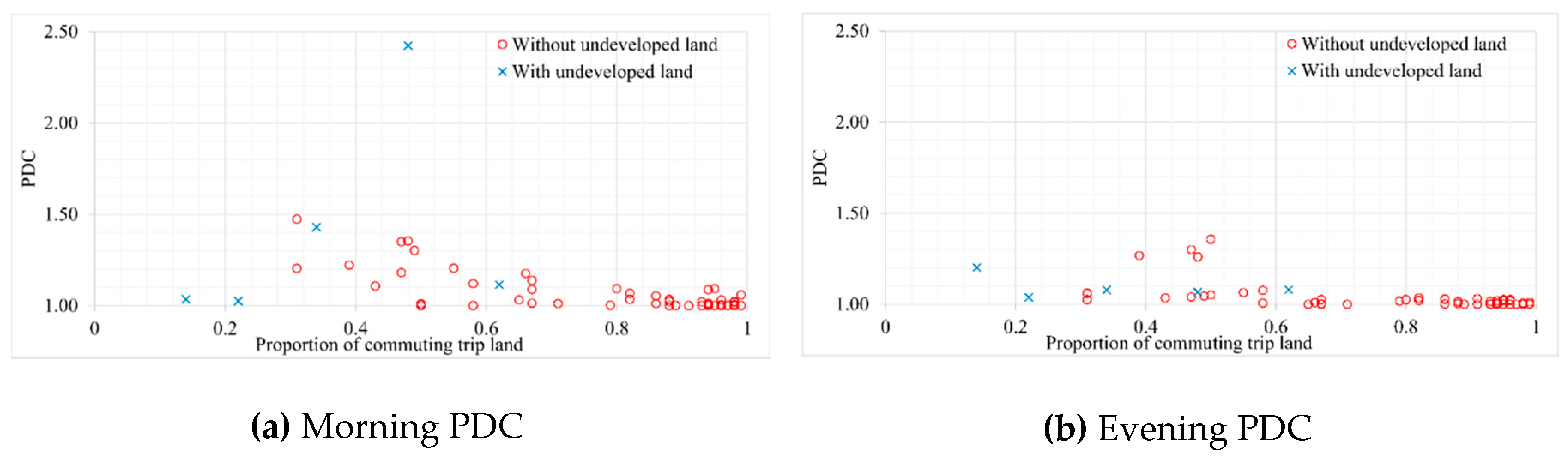
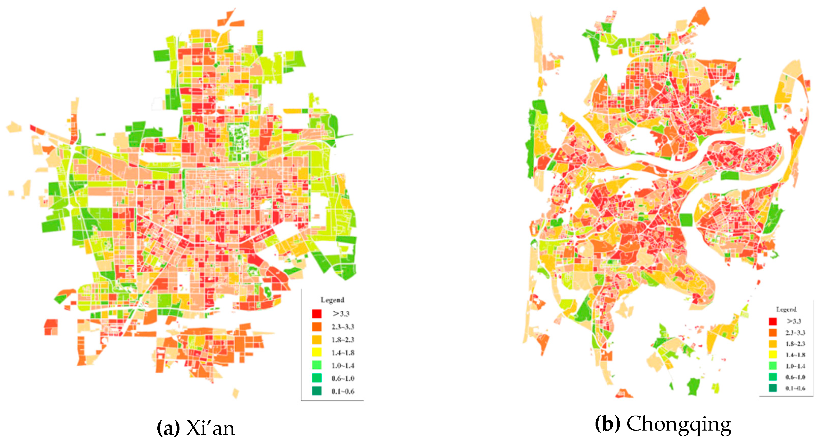
Analyzing the relationship between PDC and the proportion of commuting trip land in Xi’an shows that if the proportion of commuting trip land is below 0.5, most PDCs are over 1.10. If the proportion of commuter travel land is no less than 0.5, most PDCs are under 1.10. The distribution of plot ratio in Xi’an and Chongqing [53] is shown in Figure 9. The plot ratio in Xi’an decreases from the city center to the periphery areas because it is a plain city. The high plot ratio in Chongqing is distributed in many areas because it is a mountainous city and the land is separated by mountains and rivers. Thus, the morphological structure of the two cities are not the same. If the relationship between PDCs and the proportion of commuting trip land in Chongqing is similar to Xi’an, the results will provide some universal applicability. The relationship between rail transit station PDC and the proportion of commuting trip land in Chongqing is analyzed in the following section.
The data in Chongqing were taken 4 May 2016 (Wednesday), and included 83 stations from Line 1, Line 3, and Line 6. Before conducting statistical evaluation, the stations with undeveloped land were removed from the sample, and 52 stations remained. The PDC and proportion of commuting trip land of Chongqing rail transit stations are provided in Table 7.
The statistical relationship between rail transit station PDCs and the proportion of commuting trip land in Chongqing is shown in Table 8. As seen in the table, 78.26% of stations where the proportion of commuting trip land is more than 0.50 have morning PDCs under 1.10, and 89.13% have evening PDCs under 1.10. The stations where the proportion of commuting trip land is less than 0.50 have polarized morning PDCs, in which 33.33% of station PDCs are under 1.10, and 66.67% of station PDCs are over 1.10. All stations with a proportion of commuting trip land that is less than 0.50 have evening PDCs over 1.20. This result is in accordance with Xi’an in that most of the urban rail transit stations’ peak hours were completely consistent with that of the cities when their proportions of commuting trip land were more than 0.50, and most of the urban rail transit stations’ peak hours were not completely consistent with that of the cities when their proportions of commuting trip land were less than 0.50. However, in Chongqing, the deviation of peak hours is high in the evening, and this result is not coincident with the result in Xi’an.

5. Conclusions

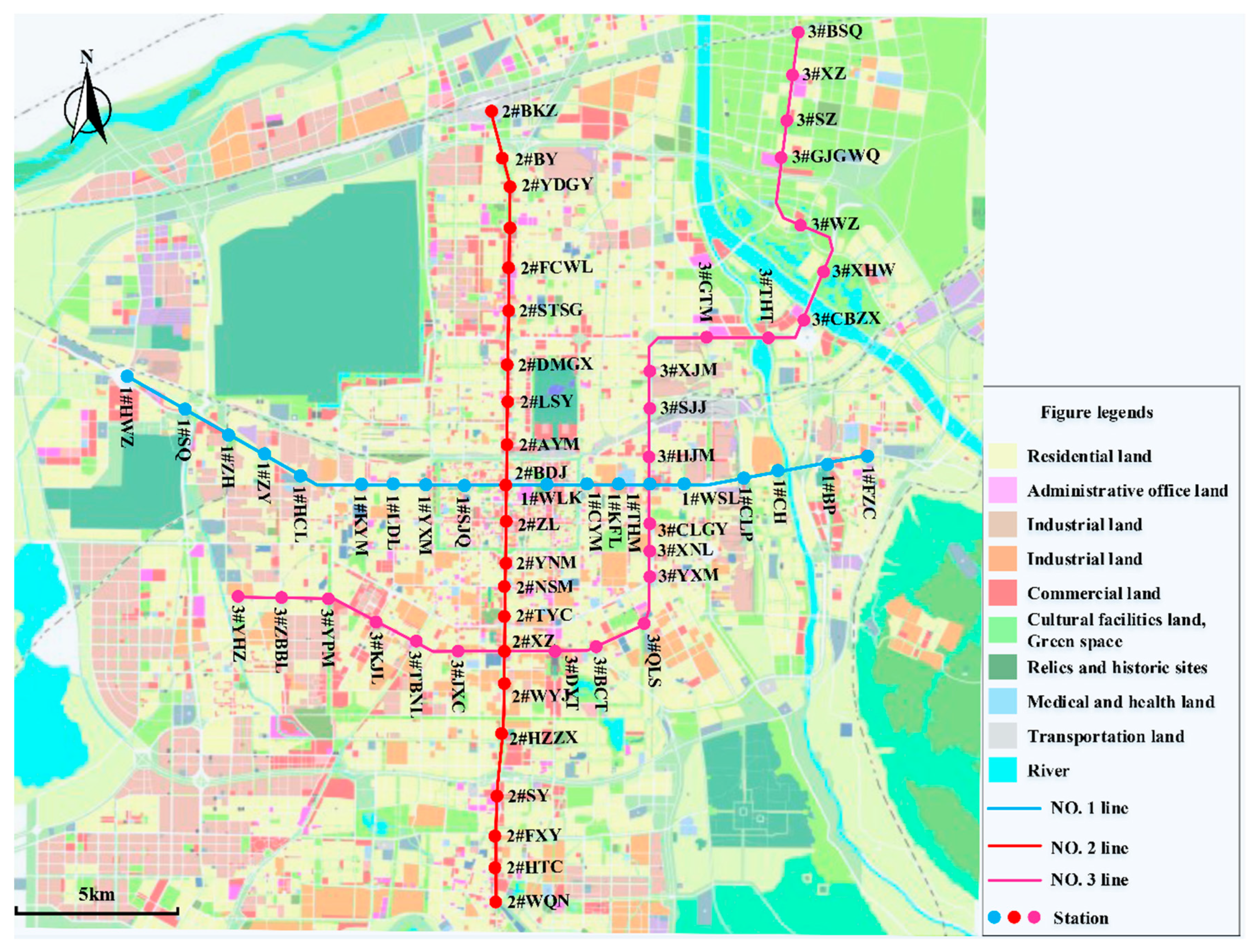
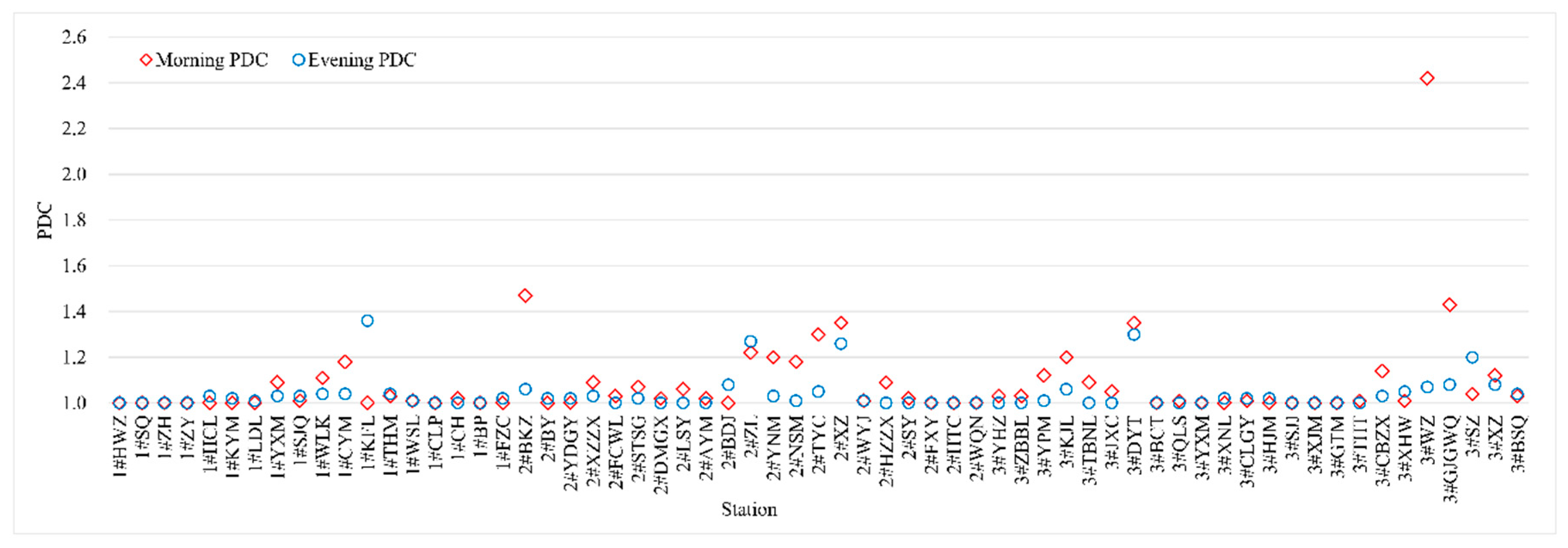
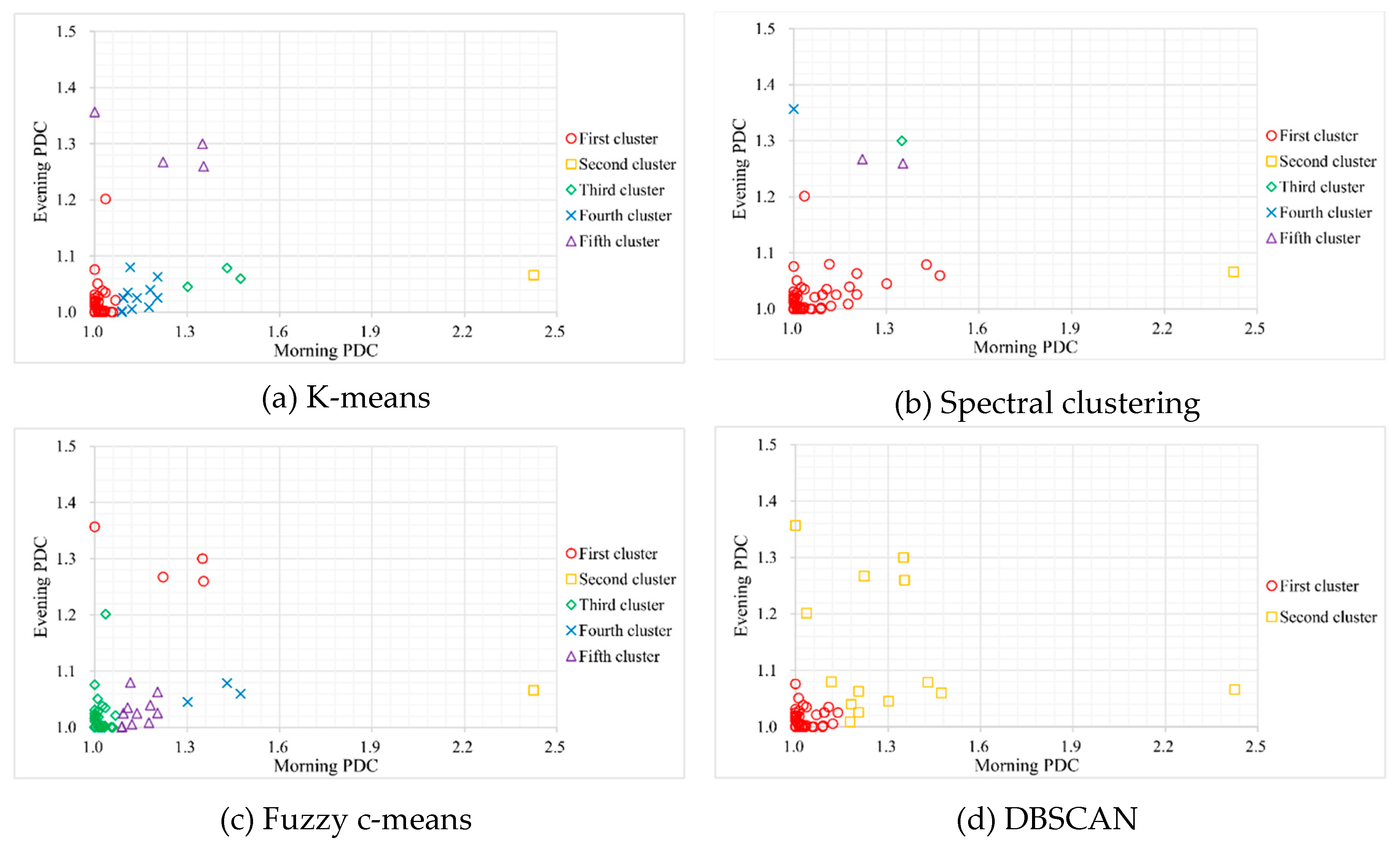
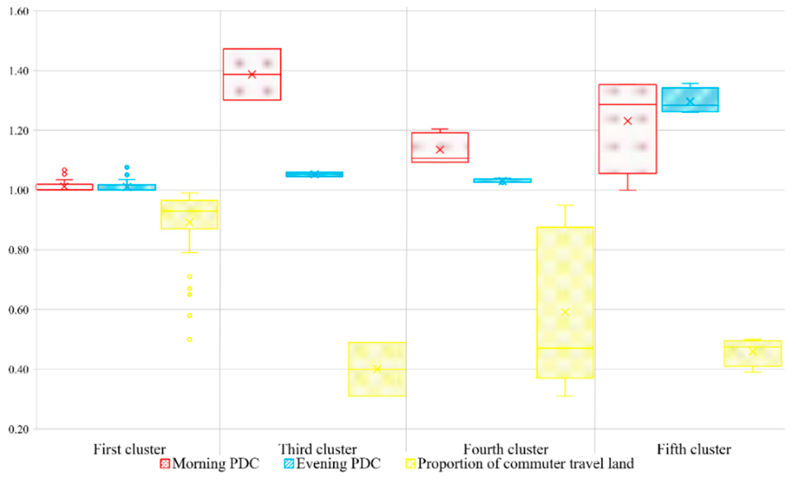
This paper investigated the inconsistencies of passenger flow volume between station peak hours and city peak hours for 63 rail transit stations in Xi’an. To verify the results, 53 rail transit stations in Chongqing were also analyzed. The key findings are as follows:
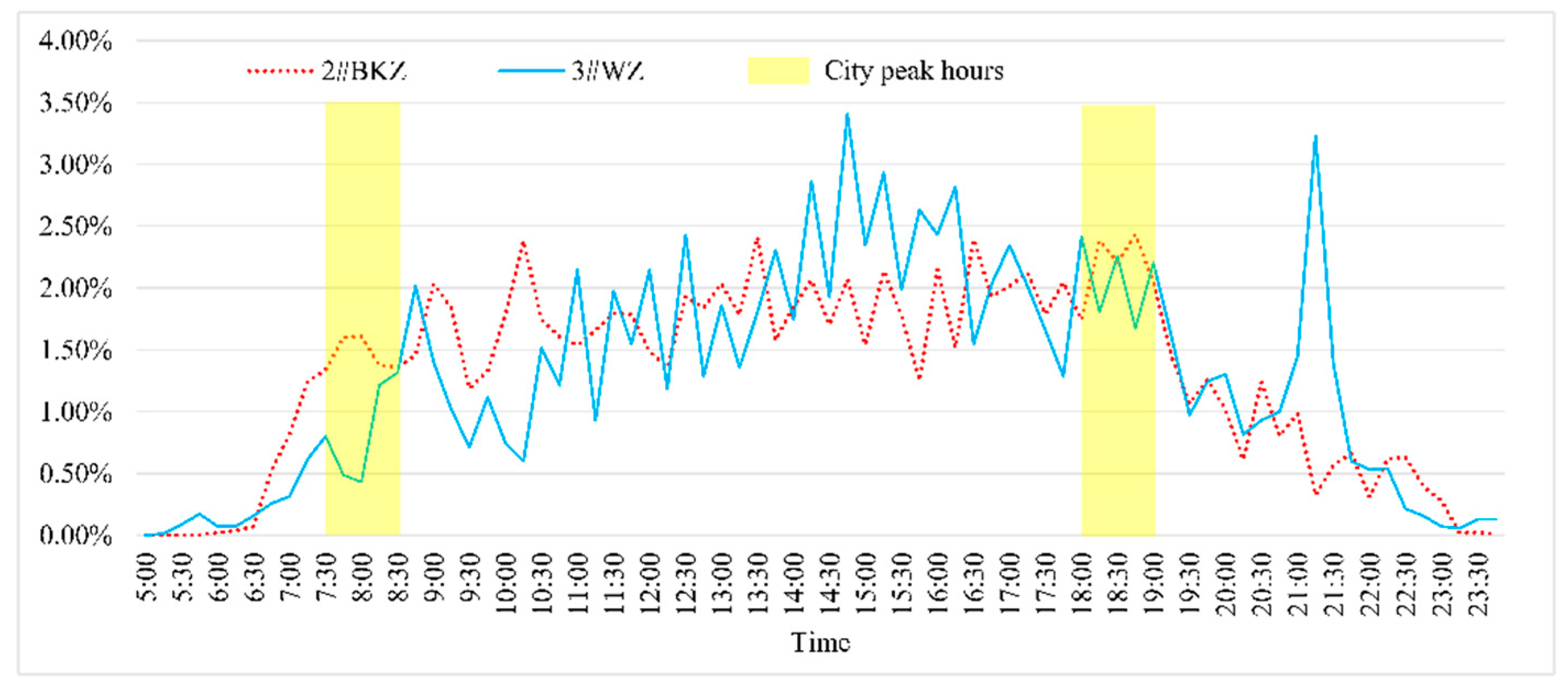
  • Current ridership data in Xi’an and Chongqing illustrate the phenomenon that urban rail transit station peak hours are not completely consistent with that of the cities. Thus, using station ridership data in peak hour to design stations may produce some errors.
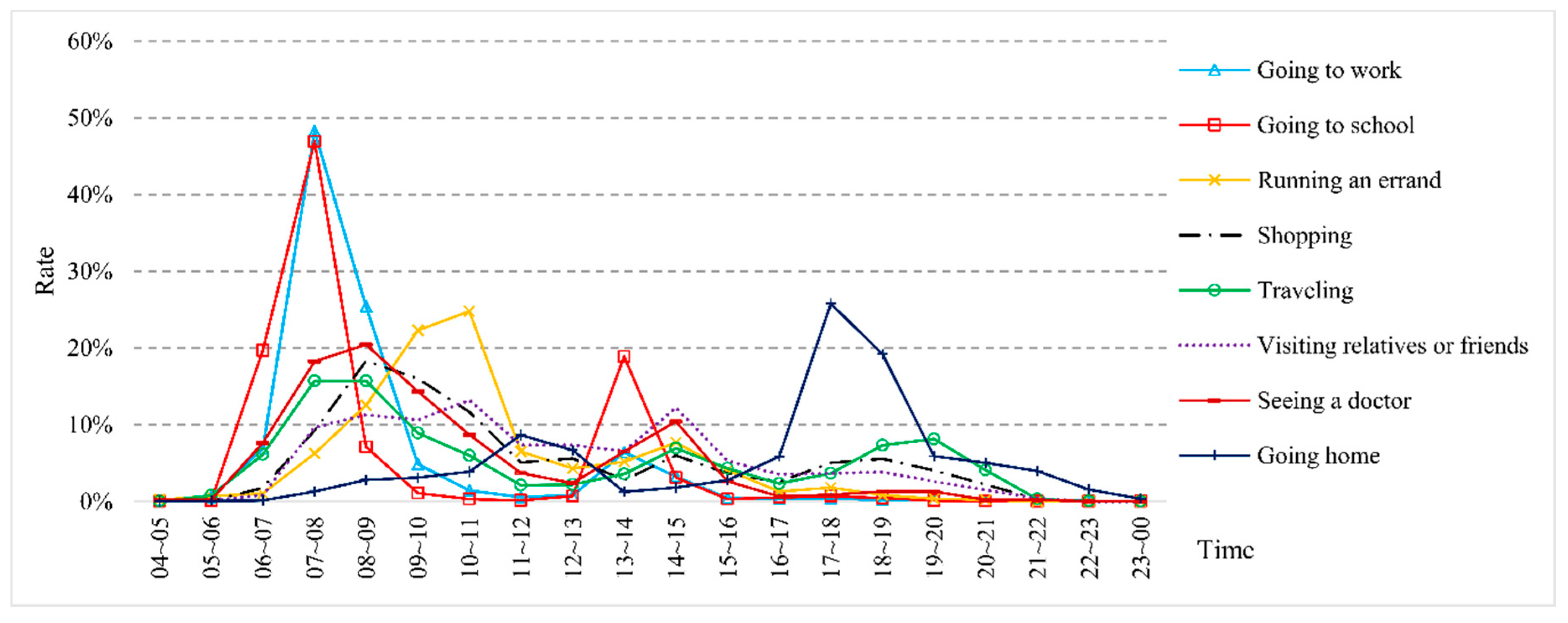
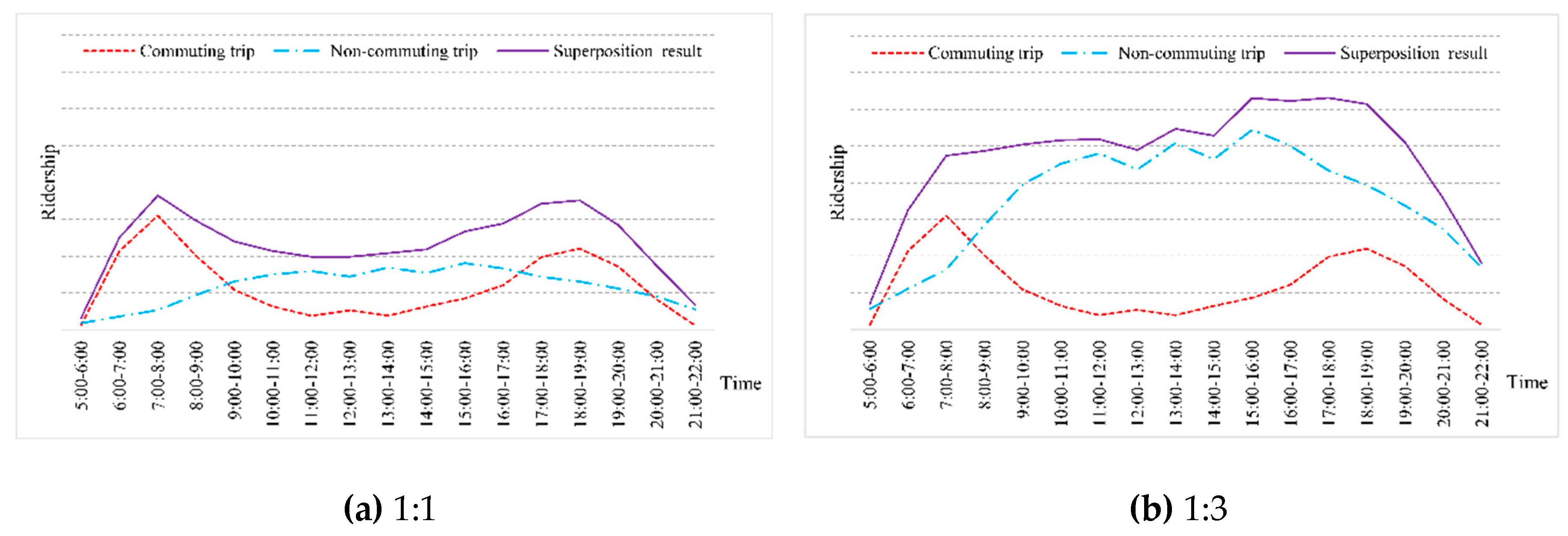
  • The temporal distribution of the station is the superposition of different temporal distributions of the purpose determined by land-use attributes. Temporal distribution is determined by the proportion of different land-use attributes, and also dictates if the station peak hour is consistent with the city peak hour or not.
  • Peak deviation coefficient (PDC) was introduced to describe the inconsistencies of passenger flow volume between station peak hours and city peak hours. It is the ratio between the predicted volume in the station’s own peak hour, and the city’s peak hour. When designing a station, only the predicted boarding and alighting volume in city peak hours is required. The boarding and alighting volume of the station can then be established by multiplying by PDC.
  • The relationship between PDC and land-use attributes was also determined. For the stations in Xi’an without undeveloped land, 92.00% of stations with a proportion of commuter travel land over 0.50 have morning PDCs under 1.10, and 98.00% of the stations have evening PDCs under 1.10. All stations with a proportion of commuter travel land less than 0.50 have morning PDCs over 1.10. The stations where the proportion of commuter travel land is less than 0.50 have polarized evening PDCs. In this case, 62.50% of the stations have PDCs under 1.10, and 37.5% of the stations have PDCs over 1.20.
  • The results from Chongqing were in accordance with Xi’an in that most metro station peak hours are completely consistent with that of the city when their proportions of commuter travel land are more than 0.50, and most metro station peak hours are not completely consistent with that of the city when their proportions of commuter travel land are less than 0.50.
By determining the law between PDC and land-use attributes, this paper provides a mechanism to select a suitable amplification coefficient when designing rail transit stations based on passenger flow forecasting.
The shortcomings of this research are acknowledged as follows. Firstly, the PDCs are not the same every day, and the rangeability for each station is also different, indicating that other influencing factors which change daily also influence the PDCs. Secondly, this paper only considers the boarding and alighting volume, but does not take transferring passengers in the interchange stations into consideration. The occurrence of peak hour transferring volume is the result of the accumulation from upstream stations, and is influenced by the peak hours of these stations boarding and alighting volume. Further research focusing on these issues is required.

Author Contributions

Conceptualization, L.Y.; methodology, L.Y.; software, Q.C.; validation, L.Y.; formal analysis, L.Y. and K.C.; investigation, L.Y.; resources, K.C.; data curation, Q.C.; writing—original draft preparation, L.Y.; writing—review and editing, Q.C.; visualization, Q.C.; funding acquisition, K.C.

Funding

This research was funded by the National Natural Science Foundation of China, grant number 71871027.

Acknowledgments

Here we acknowledge the anonymous reviewers and authors of cited papers for their detailed comments, without which this work would not have been possible.

Conflicts of Interest

The authors declare no conflict of interest.

References

  1. Tobin, R.L.; Friesz, T.L. Sensitivity Analysis for Equilibrium Network Flow. Transp. Sci. 1998, 22, 100–105. [Google Scholar] [CrossRef]
  2. Voshva, P. Application of cross-nested LOGIT model to mode choice in Tel Aviv, Israel, metropolitan area. Transp. Res. Rec. 1998, 1607, 7–15. [Google Scholar]
  3. He, R.-B. Study on Macroscopical Models of Divinable Psaaenger Flow of Subway; Chongqing University: Chongqing, China, 2002. [Google Scholar]
  4. Ma, C.-Q.; Wang, Y.-P. Traffic Volume Forecast for Xi’an Urban Rapid Rail Transit. Urban Rapid Rail Transit 2006, 19, 24–28. [Google Scholar]
  5. An, S.-Z.; Wang, B.; Li, X.-X. Inspiration for Rail Transit Passenger Flow Forecast from the Operation of Beijing Subway Line 5. Urban Rapid Rail Transit 2008, 21, 14–18. [Google Scholar]
  6. He, N.; Ma, X.-S.; Wang, G.-X. Nanjing Subway Line1Passenger Forecasting for the Opening Period. Urban Transp. China 2009, 7, 36–44. [Google Scholar] [CrossRef]
  7. Zhang, J. Post Evaluation of Passenger Flow Forecasting in Shanghai Rail Network. Traffic Transp. 2010, 2, 101–104. [Google Scholar]
  8. Shen, J.-Y. Forecasting and Application of Rail Transit Passenger Volumes. Urban Transp. China 2008, 6, 9–15, 20. [Google Scholar] [CrossRef]
  9. Lan, P. Study on Rail Passenger Flow Forecast Model Based on the Chain of Travel’s Purpose; Beijing Jiaotong University: Beijing, China, 2009. [Google Scholar]
  10. Ma, C.-Q.; Chen, K.-M.; Wang, Y.-P. Forecasting model of urban rail transit volume. J. Chang’an Univ. Nat. Sci. Ed. 2010, 30, 69–74. [Google Scholar]
  11. Zou, W.; Lu, B.-C.; Deng, J.; Ma, Q.-L.; Qiu, S.-C.; Zhang, Q. Passenger Flow Prediction Based on Genetic Algorithms and Wavelet Neural Networks. J. Wuhan Univ. Technol. Transp. Sci. Eng. 2014, 38, 1148–1151, 1157. [Google Scholar] [CrossRef]
  12. Xiao, Y.; Liu, X.-J. Research on an Extended Feedback Four-step Algorithm in Passenger Flow Forecast of Urban Rail Transit. Urban Rapid Rail Transit 2014, 27, 48–51. [Google Scholar] [CrossRef]
  13. Jiang, Y.-K. Passenger Flow Forecast for Rail Transit Lines Extended to Suburb. Urban Rapid Rail Transit 2009, 22, 44–48. [Google Scholar]
  14. Li, X.-M.; Zeng, M.-G.; Huang, G.-Z. Passenger Flow Forecast for Intercity Rail Transit Corridor Based on the Dynamic Interaction Mechanism between Traffic System and Urban Spatial Structure. China Railw. Sci. 2009, 30, 118–123. [Google Scholar]
  15. Wu, S.-M. Research on Passenger Flow Forecast Model of Multi-Level Rail Transit in Dense City Group; Harbin Institute of Technology: Harbin, China, 2014. [Google Scholar]
  16. Wang, H.-J.; Cao, Y.-Q. Study on the Methods to Forecast Passenger Flow of Intercity Rail Transit for Urban Agglomeration. J. Railw. Sci. Eng. 2015, 12, 1520–1525. [Google Scholar] [CrossRef]
  17. Yu, W.; Chen, M.-C. Forecasting the short-term metro passenger flow with empirical mode decomposition and neural networks. Transp. Res. Part C Emerg. Technol. 2012, 21, 148–162. [Google Scholar] [CrossRef]
  18. Morales, F.; Gifre, L.; Paolucci, F.; Ruiz, M.; Cugini, F.; Castoldi, P.; Velasco, L. Dynamic Core VNT Adaptability Based on Predictive Metro-Flow Traffic Models. J. Opt. Commun. Netw. 2017, 9, 1202–1211. [Google Scholar] [CrossRef]
  19. Li, L.-C.; Wang, Y.-G.; Zhong, G.; Zhang, J.; Ran, B. Short-to-medium Term Passenger Flow Forecasting for Metro Stations using a Hybrid Model. KSCE J. Civ. Eng. 2018, 22, 1937–1945. [Google Scholar] [CrossRef]
  20. Liu, S.-S.; Yao, E.-J. Holiday Passenger Flow Forecasting Based on the Modified Least-Square Support Vector Machine for the Metro System. J. Transp. Eng. Part A Syst. 2017, 143, 04016005. [Google Scholar] [CrossRef]
  21. Bai, L. Urban Rail Transit Normal and Abnormal Short-term Passenger Flow Forecasting Method. J. Transp. Syst. Eng. Inf. Technol. 2017, 17, 127–135. [Google Scholar] [CrossRef]
  22. He, Z.-Q. Study of Prediction Methods of Passenger Flow in Different Directions of Urban Rail Transit Station. Transp. Sci. Technol. 2012, 119–122. [Google Scholar] [CrossRef]
  23. Li, B.-B.; Yao, E.-J.; Liu, S.-S.; Jin, F.-L. Impact Analysis of Station Surrounding Area’s Land Use on Urban Rail Passenger Flow Distribution Based on Fuzzy Clustering. In Proceedings of the 4th International Conference on Energy and Environmental Protection, Shenzhen, China, 2–4 June 2015; pp. 44–48. [Google Scholar]
  24. Deng, J. Interactive Relationship between Ridership Characteristics at Subway Station and Surrounding Land-Use: A Case Study in Beijing; Beijing Jiaotong University: Beijing, China, 2015. [Google Scholar]
  25. Yao, E.-J.; Cheng, X.; Liu, S.-S.; Zhang, R. Accessibility-based Forecast on Passenger Flow Entering and Departing Existing Urban Railway Stations. J. China Railw. Soc. 2016, 220–222. [Google Scholar] [CrossRef]
  26. Tsang, C.W.; Ho, T.K. Passenger flow and station facilities modelling for metro station layout design. In Proceedings of the 4th International Conference on Traffic and Transportation Studies, Dalian, China, 2–4 August 2004; pp. 663–671. [Google Scholar]
  27. Wang, L.-H. Design of Platform of Subway Station. North Commun. 2008, 38, 1–7. [Google Scholar] [CrossRef]
  28. Zhong, C.; Batty, M.; Manley, E.; Wang, J.-Q.; Wang, Z.-J.; Chen, F.; Schmitt, G. Variability in Regularity: Mining Temporal Mobility Patterns in London, Singapore and Beijing Using Smart-Card Data. PLoS ONE 2016, 11, e149222. [Google Scholar] [CrossRef] [Green Version]
  29. Ma, X.-L.; Zhang, J.-Y.; Ding, C.; Wang, Y.-P.; Ma, X.; Zhang, J.; Ding, C.; Wang, Y. A geographically and emporally weighted regression model to explore the spatiotemporal influence of built environment on transit ridership. Comput. Environ. Urban Syst. 2018, 70, 113–124. [Google Scholar] [CrossRef]
  30. Shi, Z.-B.; Zhang, N.; Liu, Y.; Xu, W. Exploring Spatiotemporal Variation in Hourly Metro Ridership at Station Level: The Influence of Built Environment and Topological Structure. Sustainability 2018, 10, 4564. [Google Scholar] [CrossRef]
  31. Zhu, Y.-D.; Chen, F.; Wang, Z.-J.; Deng, J. Spatio-temporal analysis of rail station ridership determinants in the built environment. Transportation 2018. [Google Scholar] [CrossRef]
  32. Shen, J.-Y. Simplified Calculation for the Width of on and off Region of Station Platform. Urban Rapid Rail Transit 2008, 5, 9–12. [Google Scholar]
  33. Kudarov, R.S. Modelling basic constituents of incoming metro passenger flow during rush hours. Vestnik 2009, 1, 138–142. [Google Scholar]
  34. Gu, L.-P.; Ye, X.-F. Study on the in and out passenger flow during peak hours of the rail transit station in Osaka. Compr. Transp. 2014, 2, 57–61. [Google Scholar]
  35. Cheng, Y.; Ye, X.-F.; Wang, Z.; Zhou, L.-F. Forecasting Model of Peak-Period Station Origin-Destination Matrix in Urban Rail Transit Systems. J. Tongji Univ. Nat. Sci. 2018, 46, 346–353. [Google Scholar] [CrossRef]
  36. GB/T51150-2016, Code for Prediction of Urban Rail Transit Ridership. Available online: http://www.zzguifan.com/webarbs/book/92970/3172164.shtml (accessed on 8 March 2019).
  37. Roess, R.P.; Prassas, E.S.; McShane, W.R. Traffic Engineering; Pearson/Prentice Hall: Upper Saddle River, NJ, USA, 2004; ISBN 0-13-142471-8. [Google Scholar]
  38. Teng, S.-H. Analysis of the Relationship between Land Use, Development, and Construction near a Rail Traffic Station and Passenger Flow Volume: The Case of Tianjin Metro Line 1. In Proceedings of the 3rd International Conference on Civil Engineering, Architecture and Building Materials, Jinan, China, 24–26 May 2013; pp. 357–360. [Google Scholar] [CrossRef]
  39. Li, J.-F.; Yang, G.-H.; Zou, J.-Y.; Chai, D. Forecasting Method of Urban Rail Transit Ridership at Station-level Based on Population Variable in Circle Group. J. Tongji Univ. Nat. Sci. 2015, 43, 423–429. [Google Scholar] [CrossRef]
  40. Liu, W.-S.; Zhao, C.-F.; Tan, Q.; Liao, J. Model and Algorithm of Optimizing to Integrated Land-use of Rail Station Areas Based on Two-way Balanced Passenger Flow. Syst. Eng. 2015, 33, 136–140. [Google Scholar]
  41. Yao, E.-J.; Li, B.-B.; Liu, S.-S.; Zhang, Y.-S. Forecast of Passenger Flow Distribution among Urban Rail Stations Considering the Land-use Matching Degree. J. Transp. Syst. Eng. Inf. Technol. 2015, 15, 107–113. [Google Scholar]
  42. Saxena, A.; Prasad, M.; Gupta, A.; Bharill, N.; Patel, O.P.; Tiwari, A.; Er, M.J.; Ding, W.; Lin, C.-T. A Review of Clustering Techniques and Developments. Neurocomputing 2017, 267, 664–681. [Google Scholar] [CrossRef]
  43. MacQueen, J.B. Some methods for classification and analysis of multivariate observations. Berkeley Symp. Math. Statist. Prob. 1967, 1, 281–297. [Google Scholar]
  44. Ulrike, V.L. A tutorial on spectral clustering. Stat. Comput. 2007, 17, 395–416. [Google Scholar] [Green Version]
  45. Yu, L.-J.; Li, Y.; Chen, K.-M. Classification Method for Urban Rail Stations Using Spectral Clustering. J. Transp. Inf. Saf. 2014, 32, 122–125, 129. [Google Scholar]
  46. Rui, X.; Donald, W. Survey of clustering algorithms. IEEE Trans. Neural Netw. 2005, 16, 645–678. [Google Scholar]
  47. Wu, Y.; Yang, K.; Zhang, J.-Z. Using DBSCAN clustering algorithm in spam identifying. In Proceedings of the 2nd International Conference on Education Technology and Computer, Shanghai, China, 22–24 June 2010; pp. 398–402. [Google Scholar] [CrossRef]
  48. Tepwankul, A.; Maneewongwattana, S. U-DBSCAN: A Density-Based Clustering Algorithm for Uncertain Objects. In Proceedings of the 26th IEEE International Conference on Data Engineering, Long Beach, CA, USA, 1–6 March 2010; pp. 136–143. [Google Scholar] [CrossRef]
  49. Wang, Y.-Q.; Chen, Z.-N.; Qin, S.-J. Research on the structural relationship of metro accessibility, passenger flows and retail business in metro sites: A case study of Guangzhou. Hum. Geogr. 2015, 30, 66–71. [Google Scholar]
  50. Wang, S.-W.; Sun, L.-S.; Hao, S.-Y.; Rong, J. Station level transit ridership direct estimation model based on precise land use. J. Transp. Syst. Eng. Inf. Technol. 2015, 15, 37–43. [Google Scholar]
  51. Kuby, M.; Barranda, A.; Upchurch, C. Factors influencing lightrail station boardings in the United States. Transp. Res. Part A Policy Pract. 2004, 38, 223–247. [Google Scholar] [CrossRef]
  52. El-Geneidy, A.M.; Tetreault, P.; Surprenant-Legault, J. Pedestrian access to transit: Identifying redundancies and gaps using a variable service area analysis. In Proceedings of the Transportation Research Board 89th Annual Meeting, Washing, DC, USA, 10–14 January 2010. [Google Scholar]
  53. Refined Scale Urban Morphology in China. Available online: https://geohey.com/apps/dataviz/2ef6b66a08da4103ae81b6a715fbaae9/share?ak=ZmYzNmY0ZWJhYjcwNGU2ZGExNDgxMWUxNmZiOWNhNGY (accessed on 29 April 2019).
Figure 1. Temporal distributions of trip purpose. The y-axis means the ratio of trips in one hour to the all-day trips.
Sustainability 11 02733 g001
Figure 2. Schematic diagram of the superposition of the commuting trip and non-commuting trip at different trip proportions.
Sustainability 11 02733 g002
Figure 3. Temporal distribution of two stations.
Sustainability 11 02733 g003
Figure 4. Urban rail transit networks in Xi’an.
Sustainability 11 02733 g004
Figure 5. PDCs of Xi’an urban rail transit stations (PDCs is the plural form of PDC).
Sustainability 11 02733 g005
Figure 6. Results of the classification.
Sustainability 11 02733 g006
Figure 7. Relationship between PDCs and the commuting trip land proportion.
Sustainability 11 02733 g007
Figure 8. Box figure of PDC and land use of every cluster.
Sustainability 11 02733 g008
Figure 9. Distribution of plot ratio in Xi’an and Chongqing.
Sustainability 11 02733 g009
Table 1. Statistics of the deviation of peak hours for urban rail transit stations in the two cities.
CityCity Peak HourLines’ NameTotal Number of StationsNumber of Deviation StationsDeviation Proportion
Xi’an, China07:30~08:30NO.118844.44%
NO.2211676.19%
NO.3241875.00%
Chongqing, China08:00~09:00NO.1231669.57%
NO.3362569.44%
NO.6241770.83%
Table 2. Statistics of PDC of each station.
StationPDCStationPDC
MorningEveningMorningEvening
1#HWZ1.001.002#XZ1.351.26
1#SQ1.001.002#WYJ1.011.01
1#ZH1.001.002#HZZX1.091.00
1#ZY1.001.002#SY1.021.00
1#HCL1.001.032#FXY1.001.00
1#KYM1.001.022#HTC1.001.00
1#LDL1.001.012#WQN1.001.00
1#YXM1.091.033#YHZ1.031.00
1#SJQ1.011.033#ZBBL1.031.00
1#WLK1.111.043#YPM1.121.01
1#CYM1.181.043#KJL1.201.06
1#KFL1.001.363#TBNL1.091.00
1#THM1.031.043#JXC1.051.00
1#WSL1.011.013#DYT1.351.30
1#CLP1.001.003#BCT1.001.00
1#CH1.021.003#QLS1.011.00
1#BP1.001.003#YXM1.001.00
1#FZC1.001.023#XNL1.001.02
2#BKZ1.471.063#CLGY1.011.02
2#BY1.001.023#HJM1.001.02
2#YDGY1.001.023#SJJ1.001.00
2#XZZX1.091.033#XJM1.001.00
2#FCWL1.031.003#GTM1.001.00
2#STSG1.071.023#THT1.011.00
2#DMGX1.021.003#CBZX1.141.03
2#LSY1.061.003#XHW1.011.05
2#AYM1.021.003#WZ2.421.07
2#BDJ1.001.083#GJGWQ1.431.08
2#ZL1.221.273#SZ1.041.20
2#YNM1.201.033#XZ1.121.08
2#NSM1.181.013#BSQ1.031.04
2#TYC1.301.05
Table 3. Results of partition of land use.
CategoriesLand Use
Commuting trip landHousing landResidential land
Working landAdministrative office land, Industrial land
Educational landEducational and scientific research land
Non-commuting trip landRecreation landCommercial land, Cultural facilities land, Relics and historic sites, Square land
Health facilities landMedical and health land
Transportation hub landTransportation land
Undeveloped landGreen space
Table 4. Built environment of each rail transit station.
StationCommuting Trip Land (×104 m2)Non-Commuting Trip Land (×104 m2)Proportion of Commuting Trip Land
Housing LandWorking LandEducational LandRecreation LandHealth Facilities LandTransportation HubUndeveloped Land
1#HWZ701.67.2 55.26.6 0.059.20.00.92
1#SQ643.4112.6 17.650.2 0.00.00.00.94
1#ZH472.896.8 0.072.2 0.00.00.00.89
1#ZY449.464.8 0.025.6 0.00.00.00.95
1#HCL517.091.4 31.845.4 0.020.60.00.91
1#KYM443.699.6 0.038.2 0.00.00.00.93
1#LDL526.846.2 6.26.6 2.60.00.00.99
1#YXM673.289.8 0.037.6 0.00.00.00.95
1#SJQ396.431.6 7.063.8 5.40.00.00.86
1#WLK139.833.6 22.8130.4 121.80.00.00.44
1#CYM134.835.2 21.6179.8 33.60.00.00.48
1#KFL176.243.4 30.6123.6 133.00.00.00.50
1#THM604.60.0 33.2119.2 14.20.00.00.83
1#WSL564.457.6 0.88.8 0.00.00.00.99
1#CLP620.225.6 21.236.4 28.80.00.00.91
1#CH424.861.6 35.413.6 0.00.00.00.97
1#BP593.059.2 0.062.2 0.00.00.00.91
1#FZC582.422.0 0.09.8 69.481.60.00.79
2#BKZ57.816.4 0.011.6 0.0151.60.00.31
2#BY597.467.2 0.032.6 0.00.00.00.95
2#YDGY783.214.6 36.447.0 0.00.00.00.95
2#XZZX270.689.0 0.092.4 0.00.00.00.80
2#FCWL1116.480.0 4.4157.2 0.00.00.00.88
2#STSG972.692.4 7.8200.4 49.60.00.00.81
2#DMGX1039.027.2 0.0112.6 28.40.00.00.89
2#LSY1231.20.0 10.618.8 0.00.00.00.99
2#AYM567.60.0 47.412.2 0.00.00.00.98
2#BDJ505.681.0 13.0251.8 188.60.00.00.58
2#ZL456.816.0 25.6657.4 101.00.00.00.40
2#YNM172.080.6 0.0557.0 0.00.00.00.31
2#NSM291.0121.2 14.8197.8 17.60.00.00.66
2#TYC159.60.0 3.8167.0 0.00.00.00.49
2#XZ348.088.0 74.2553.8 0.00.00.00.48
2#WYJ283.440.4 255.242.2 0.00.00.00.93
2#HZZX610.847.0 4.0321.8 0.00.00.00.67
2#SY740.075.6 59.061.6 0.00.00.00.93
2#FXY933.455.2 70.263.6 0.00.00.00.94
2#HTC1266.4146.6 0.067.2 0.00.00.00.95
2#WQN1053.642.8 0.074.8 18.00.00.00.92
3#YHZ74.84.9 0.043.4 0.00.00.00.65
3#ZBBL1246.20.0 11.152.0 0.00.00.00.96
3#YPM370.0121.6 6.0359.2 0.00.00.00.58
3#KJL285.680.2 20.5311.2 0.00.00.00.55
3#TBNL1528.676.8 19.793.0 4.80.00.00.95
3#JXC617.30.0 7.294.0 11.20.00.00.85
3#DYT150.60.0 16.4191.2 0.00.00.00.47
3#BCT785.042.0 0.022.0 0.00.00.00.97
3#QLS184.813.0 11.2102.7 0.00.00.00.67
3#YXM822.20.0 13.08.2 0.00.00.00.99
3#XNL224.00.0 78.015.6 0.00.00.00.95
3#CLGY730.00.0 39.347.7 0.00.00.00.94
3#HJM820.00.0 9.6117.6 0.00.00.00.88
3#SJJ471.060.0 0.07.0 0.00.00.00.99
3#XJM728.011.0 6.016.4 0.00.00.00.98
3#GTM372.9231.3 0.016.4 0.00.00.00.97
3#THT110.48.4 10.654.8 0.00.00.00.70
3#CBZX107.020.5 0.064.5 0.00.00.00.66
3#XHW140.20.0 4.2141.6 0.00.00.00.50
3#WZ129.60.0 0.02.6 0.00.0138.30.48
3#GJGWQ30.643.3 0.014.9 0.00.0125.90.34
3#SZ27.82.6 0.04.5 0.00.0179.60.14
3#XZ95.539.3 2.81.8 0.00.084.50.61
3#BSQ50.30.0 0.01.5 0.00.0181.00.21
Table 5. Results of partition of land use.
ItemFirst ClusterSecond ClusterThird ClusterFourth ClusterFifth Cluster
PDCMorningAverage1.012.421.401.131.23
Minimum1.00-1.301.091.00
Maximum1.07-1.471.201.35
EveningAverage1.021.071.061.031.30
Minimum1.00-1.051.001.26
Maximum1.20-1.081.081.36
Proportion of commuting trip landAll stationsAverage0.860.480.380.640.46
Minimum0.14-0.310.310.39
Maximum0.99-0.490.950.50
Undeveloped land not existsAverage0.89-0.400.640.46
Minimum0.50-0.310.310.39
Maximum0.99-0.490.950.50
Undeveloped land existsAverage0.180.480.340.62-
Minimum0.14----
Maximum0.22----
Table 6. Statistical distribution of the stations.
Proportion of Commuting Trip Land<0.5≥0.5
PDCMorningEveningMorningEvening
(1.00, 1.10)0.00%62.50%92.00%98.00%
(1.10, 1.20)37.50%0.00%8.00%0.00%
(1.20, 1.30)25.00%37.50%0.00%0.00%
(1.30, +∞)37.50%0.00%0.00%2.00%
Table 7. The PDC and proportion of commuting trip land of Chongqing urban rail transit stations.
StationMorning PDCEvening PDCProportion of Commuting Trip LandStationMorning PDCEvening PDCProportion of Commuting Trip Land
1#SB1.071.070.813#HQHG1.061.100.90
1#CQK1.171.060.933#JZL1.001.050.97
1#LSM1.111.110.873#ZJYZ1.001.000.95
1#SPB1.001.060.893#SZP1.001.040.97
1#XLK1.081.100.883#JY1.091.010.98
1#SQP1.001.020.973#JTL1.201.100.97
1#XTZ1.021.020.923#CP1.151.040.94
1#SYL1.001.040.883#CFL1.001.001.00
1#DP1.001.050.943#HX1.051.190.96
1#EL1.001.000.663#SL1.161.100.90
1#LLK1.011.000.723#BJ1.251.620.49
1#QXG1.021.010.963#JBJC1.411.220.00
1#JCK1.001.000.783#SFQ1.181.520.48
1#XSZ1.001.000.893#GBH1.001.101.00
3#JZ1.101.000.896#BP1.061.060.80
3#XTW1.191.060.846#ZYB1.191.100.55
3#QL1.131.000.906#GDY1.061.100.98
3#BGL1.091.050.916#RJB1.041.050.79
3#ET1.001.000.936#DLS1.001.000.85
3#LGL1.001.000.896#HHY1.001.000.83
3#WGL1.201.310.506#HNB1.191.080.94
3#SGL1.051.110.906#HTD1.002.110.47
3#NP1.001.110.946#JBC1.151.200.86
3#GM1.011.050.876#LJP1.083.940.31
3#HXJ1.001.010.886#CSQ1.041.000.90
3#GYQ1.001.040.936#CY1.001.000.87
Table 8. Statistical distribution of the stations in Chongqing.
Proportion of Commuting Trip Land<0.5≥0.5
PDCMorningEveningMorningEvening
(1.00, 1.10)33.33%0.00%78.26%89.13%
(1.10, 1.20)33.33%0.00%21.74%10.87%
(1.20, 1.30)16.67%16.67%0.00%0.00%
(1.30, +∞)16.67%83.33%0.00%0.00%

