Hybrid Forecasting Model for Short-Term Electricity Market Prices with Renewable Integration

 ,
,  ,
, 

Abstract
1. Introduction
2. Proposed Hybrid Probabilistic Forecasting Model (HPFM)
2.1. Wavelet Transforms (WT)
2.2. Hybrid Particle Swarm Optimization (DEEPSO)
- Position:
- Velocity:
- Particle Weights Mutation:
- Current Best Position with Normal Distribution
- Differential Set for Particle Crossover:
2.3. Adaptive Neuro-Fuzzy Inference System (ANFIS)
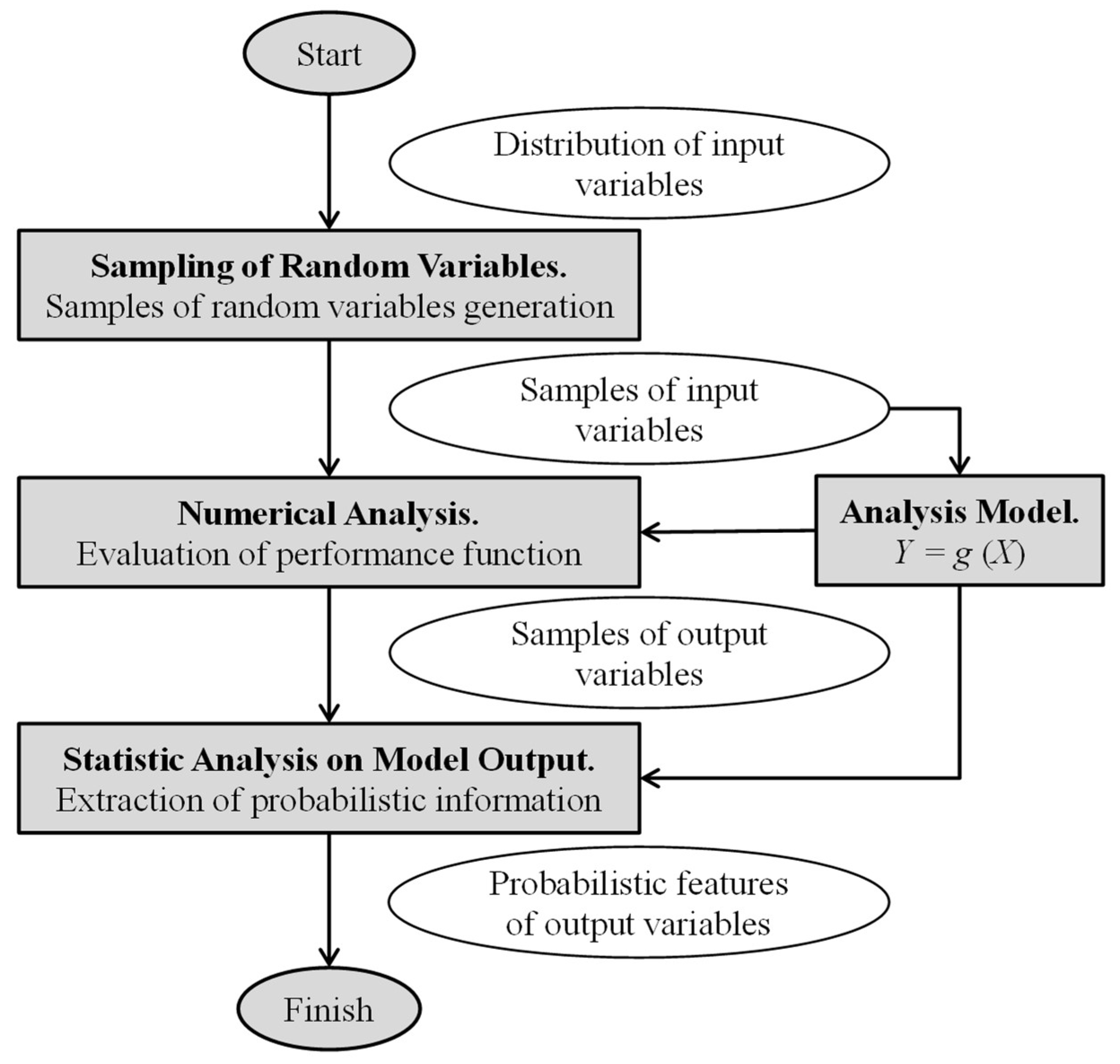
2.4. Monte-Carlo Simulation (MCS)
- The mean:
- The variance:
- The probability of failure expression in case ofwhere:
2.5. Probabilistic Hybrid Forecasting Model (PHFM)
- Step 1: Start the PHFM model with a historical data of EMP, taking as window frames the forecasting time-frame (168 h for each set chosen);
- Step 2: Select the historical data that will be decomposed by the WT;
- Step 3: Select the parameters of the DEEPSO (Table 1);
- Step 4: Select the set of weeks that will be used in DEEPSO to obtain the necessary features to tuning and increase the performance of the ANFIS model;
- Step 5: Select the parameters of the ANFIS (Table 1);
- Step 6: Select the inputs of each iteration of the ANFIS method;
- Step 7: Calculate the forecasting errors with the different error measurements criterions to authenticate the advances of the proposed PHFM model:
- ▪
- Step 7.1: If the criterion error goal is not achieved, start Step 7 again;
- ▪
- Step 7.2: If the criterion error goal is not found in Step 7, jump to Step 4 to find another set of solutions;
- ▪
- Step 7.3: If the best forecasting results are found, or the number of the iteration is reached, save the latest best record and go to Step 8;
- Step 8: Use the inverse of the WT transform to include the data previously filtered in the forecasted output;
- Step 9: Obtain the analysis result using the MCS; print the forecasting results and finish.
3. Forecasting Validation
4. Case Studies and Results
5. Conclusions
Author Contributions
Funding
Conflicts of Interest
Nomenclature and Abbreviations
| Nomenclature | |
| Scaling and translating factors, respectively in wavelet transforms. | |
| Approximation and details coefficients of order in wavelet transforms. | |
| Continuous wavelet transforms. | |
| Discrete wavelet transforms. | |
| Error variance from probabilistic hybrid forecasting model. | |
| Cumulative density function from Monte Carlo simulation. | |
| Best position for differential evolutionary particle swarm optimization. | |
| Current best position for differential evolutionary particle swarm optimization. | |
| Performances function from Monte Carlo simulation. | |
| Integer variable from Monte Carlo simulation. | |
| Particle index for differential evolutionary particle swarm optimization. | |
| Iteration index for differential evolutionary particle swarm optimization | |
| Mean absolute percentage error. | |
| Discrete wavelet transforms counterparts of scaling factors and | |
| Dimension of the input data from probabilistic hybrid forecasting model. | |
| Time index from probabilistic hybrid forecasting model. | |
| Size of the swarm for differential evolutionary particle swarm optimization. | |
| Electricity market price average results from probabilistic hybrid forecasting model. | |
| Probability of failure from Monte Carlo simulation. | |
| Probabilistic hybrid forecasting model output. | |
| Electricity market price data from probabilistic hybrid forecasting model. | |
| Complex conjugate continuous domain mother function in wavelet transforms. | |
| Wavelet transforms mother function | |
| Variance from Monte Carlo Simulation. | |
| Weekly error variance. | |
| Set of samples of random variables from Monte Carlo simulation. | |
| Length of the sampled signal in wavelet transforms. | |
| Input signal in wavelet transforms. | |
| New particle velocity in iteration for differential evolutionary particle swarm optimization. | |
| Wight parameters for differential evolutionary particle swarm optimization. | |
| Time-varying input signal in wavelet transforms (historical data series). | |
| New particle position in iteration for differential evolutionary particle swarm optimization. | |
| Differential set particle crossover for differential evolutionary particle swarm optimization. | |
| Historical data set from Monte Carlo simulation. | |
| Forecasted results from Monte Carlo simulation. | |
| Abbreviations | |
| ANFIS | Adaptive neuro-fuzzy inference system. |
| ARIMA | Auto-regressive integrated moving average. |
| CDF | Cumulative density function. |
| DEEPSO | Hybrid particle swarm optimization. |
| EMP | Electricity market prices. |
| EPA | Evolutionary particle swarm optimization algorithm. |
| FIS | Fuzzy inference system. |
| GA | Genetic algorithm. |
| HE | Hybrid evolutionary algorithm. |
| HIS | Hybrid intelligent system. |
| HPFM | Hybrid probabilistic forecasting model. |
| HPM | Hybrid particle swarm optimization model. |
| MAPE | Mean absolute percentage error. |
| MCS | Monte Carlo Simulation. |
| MICNN | Mutual information cascaded artificial neural networks. |
| NN | Artificial neural network. |
| Probability density function. | |
| PJM | Pennsylvania-New Jersey-Maryland electricity market. |
| PSO | Particle swarm optimization. |
| WT | Wavelet transforms. |
References
- Nowotarski, J.; Weron, R. Recent Advances in Electricity Price Forecasting: A Review of Probabilistic Forecasting. HSC Res. Rep. 2016, 81, 1548–1568. [Google Scholar] [CrossRef]
- Khooban, M.-H. Secondary Load Frequency Control of Time-Delay Stand-Alone Microgrids With Electric Vehicles. IEEE Trans. Ind. Electron. 2018, 65, 7416–7422. [Google Scholar] [CrossRef]
- Li, X.R.; Yu, C.W.; Ren, S.Y.; Chiu, C.H.; Meng, K. Day-Ahead Electricity Price Forecasting Based on Panel Cointegration and Particle Filter. Electr. Power Syst. Res. 2013, 95, 66–76. [Google Scholar] [CrossRef]
- Dufo-López, R.; Bernal-Agustín, J.L.; Monteiro, C. New Methodology for the Optimization of the Management of Wind Farms, Including Energy Storage. Appl. Mech. Mater. 2013, 330, 183–187. [Google Scholar] [CrossRef]
- Ren, Y.; Suganthan, P.N.; Srikanth, N. Ensemble Methods for Wind and Solar Power forecasting—A State-of-the-Art Review. Renew. Sustain. Energy Rev. 2015, 50, 82–91. [Google Scholar] [CrossRef]
- Okumus, I.; Dinler, A. Current Status of Wind Energy Forecasting and a Hybrid Method for Hourly Predictions. Energy Convers. Manag. 2016, 123, 362–371. [Google Scholar] [CrossRef]
- Yadav, A.; Peesapati, R.; Kumar, N. Electricity Price Forecasting and Classification Through Wavelet–Dynamic Weighted PSO–FFNN Approach. IEEE Syst. J. 2017, 29, 1–10. [Google Scholar]
- Jafari, M.; Malekjamshidi, Z.; Zhu, J.; Khooban, M.-H. Novel Predictive Fuzzy Logic-Based Energy Management System for Grid-Connected and Off-Grid Operation of Residential Smart Micro-Grids. IEEE J. Emerg. Sel. Top. Power Electron. 2018. [Google Scholar] [CrossRef]
- Osório, G.; Gonçalves, J.; Lujano-Rojas, J.; Catalão, J.; Osório, G.J.; Gonçalves, J.N.D.L.; Lujano-Rojas, J.M.; Catalão, J.P.S. Enhanced Forecasting Approach for Electricity Market Prices and Wind Power Data Series in the Short-Term. Energies 2016, 9, 693. [Google Scholar] [CrossRef]
- Catalão, J.P.S.; Pousinho, H.M.I.; Mendes, V.M.F. Short-Term Electricity Prices Forecasting in a Competitive Market by a Hybrid Intelligent Approach. Energy Convers. Manag. 2011, 52, 1061–1065. [Google Scholar] [CrossRef]
- Weron, R. Electricity Price Forecasting: A Review of the State-of-the-Art with a Look into the Future. Int. J. Forecast. 2014, 30, 1030–1081. [Google Scholar] [CrossRef]
- Contreras, J.; Espínola, R.; Nogales, F.J.; Conejo, A.J. ARIMA Models to Predict Next-Day Electricity Prices. IEEE Trans. Power Syst. 2003, 18, 1014–1020. [Google Scholar] [CrossRef]
- Catalão, J.P.S.; Mariano, S.J.P.S.; Mendes, V.M.F.; Ferreira, L.A.F.M. Short-Term Electricity Prices Forecasting in a Competitive Market: A Neural Network Approach. Electr. Power Syst. Res. 2007, 77, 1297–1304. [Google Scholar] [CrossRef]
- Kim, M.K. Short-Term Price Forecasting of Nordic Power Market by Combination Levenberg–Marquardt and Cuckoo Search Algorithms. IET Gener. Transm. Distrib. 2015, 9, 1553–1563. [Google Scholar] [CrossRef]
- Amjady, N.; Hemmati, M. Day-Ahead Price Forecasting of Electricity Markets by a Hybrid Intelligent System. Eur. Trans. Electr. Power 2009, 19, 89–102. [Google Scholar] [CrossRef]
- Miranian, A.; Abdollahzade, M.; Hassani, H. Day-Ahead Electricity Price Analysis and Forecasting by Singular Spectrum Analysis. IET Gener. Transm. Distrib. 2013, 7, 337–346. [Google Scholar] [CrossRef]
- Alamaniotis, M.; Bargiotas, D.; Bourbakis, N.G.; Tsoukalas, L.H. Genetic Optimal Regression of Relevance Vector Machines for Electricity Pricing Signal Forecasting in Smart Grids. IEEE Trans. Smart Grid 2015, 6, 2997–3005. [Google Scholar] [CrossRef]
- Osório, G.J.; Matias, J.C.O.; Catalão, J.P.S. Electricity Prices Forecasting by a Hybrid Evolutionary-Adaptive Methodology. Energy Convers. Manag. 2014, 80, 363–373. [Google Scholar] [CrossRef]
- Tahmasebifar, R.; Sheikh-El-Eslami, M.K.; Kheirollahi, R. Point and Interval Forecasting of Real-Time and Day-Ahead Electricity Prices by a Novel Hybrid Approach. IET Gener. Transm. Distrib. 2017, 11, 2173–2183. [Google Scholar] [CrossRef]
- Lee, D.; Shin, H.; Baldick, R. Bivariate Probabilistic Wind Power and Real-Time Price Forecasting and Their Applications to Wind Power Bidding Strategy Development. IEEE Trans. Power Syst. 2018, 33, 6087–6097. [Google Scholar] [CrossRef]
- Moreira, R.; Bessa, R.; Gama, J. Probabilistic Forecasting of Day-Ahead Electricity Prices for the Iberian Electricity Market. In Proceedings of the 2016 13th International Conference on the European Energy Market (EEM), Porto, Portugal, 6–9 June 2016; pp. 1–5. [Google Scholar]
- Rafiei, M.; Niknam, T.; Khooban, M.-H. Probabilistic Forecasting of Hourly Electricity Price by Generalization of ELM for Usage in Improved Wavelet Neural Network. IEEE Trans. Ind. Inform. 2017, 13, 71–79. [Google Scholar] [CrossRef]
- Miranda, V.; Alves, R. Differential Evolutionary Particle Swarm Optimization (DEEPSO): A Successful Hybrid. In Proceedings of the 2013 BRICS Congress on Computational Intelligence and 11th Brazilian Congress on Computational Intelligence, Ipojuca, Brazil, 8–11 September 2013; pp. 368–374. [Google Scholar]
- Rafiei, M.; Niknam, T.; Khooban, M.H. A Novel Intelligent Strategy for Probabilistic Electricity Price Forecasting: Wavelet Neural Network Based Modified Dolphin Optimization Algorithm. J. Intell. Fuzzy Syst. 2016, 31, 301–312. [Google Scholar] [CrossRef]
- Rafiei, M.; Niknam, T.; Khooban, M.H. Probabilistic Electricity Price Forecasting by Improved Clonal Selection Algorithm and Wavelet Preprocessing. Neural Comput. Appl. 2017, 28, 3889–3901. [Google Scholar] [CrossRef]
- Haque, A.U.; Mandal, P.; Meng, J.; Srivastava, A.K.; Tseng, T.-L.; Senjyu, T. A Novel Hybrid Approach Based on Wavelet Transform and Fuzzy ARTMAP Networks for Predicting Wind Farm Power Production. IEEE Trans. Ind. Appl. 2013, 49, 2253–2261. [Google Scholar] [CrossRef]
- Catalao, J.P.S.; Pousinho, H.M.I.; Mendes, V.M.F. Hybrid Wavelet-PSO-ANFIS Approach for Short-Term Electricity Prices Forecasting. IEEE Trans. Power Syst. 2011, 26, 137–144. [Google Scholar] [CrossRef]
- Kennedy, J.; Eberhart, R. Particle Swarm Optimization. In Proceedings of the ICNN’95—International Conference on Neural Networks, Perth, Australia, 27 November–1 December 1995; Volume 4, pp. 1942–1948. [Google Scholar]
- Castillo, O.; Martínez-Marroquín, R.; Melin, P.; Valdez, F.; Soria, J. Comparative Study of Bio-Inspired Algorithms Applied to the Optimization of Type-1 and Type-2 Fuzzy Controllers for an Autonomous Mobile Robot. Inf. Sci. 2012, 192, 19–38. [Google Scholar] [CrossRef]
- Soliman, O.S.; Mohamed, S.M.; Ramadan, E.A. A Bio-Inspired Memetic Particle Swarm Optimization Algorithm for Multi-Objective Optimization Problems. In Proceedings of the 2012 Third International Conference on Innovations in Bio-Inspired Computing and Applications, Kaohsiung, Taiwan, 26–28 September 2012; pp. 127–132. [Google Scholar]
- Hassan, R.; Cohanim, B.; de Weck, O.; Venter, G. A Comparison of Particle Swarm Optimization and the Genetic Algorithm. In Proceedings of the 46th AIAA/ASME/ASCE/AHS/ASC Structures, Structural Dynamics and Materials Conference, Austin, TX, USA, 18–21 April 2005; p. 1897. [Google Scholar]
- Miranda, V.; Cerqueira, C.; Monteiro, C. Training a FIS with EPSO under an Entropy Criterion for Wind Power Prediction. In Proceedings of the 2006 International Conference on Probabilistic Methods Applied to Power Systems, Stockholm, Sweden, 11–15 June 2006; pp. 1–8. [Google Scholar]
- Taieb, S.B.; Atiya, A.F. A Bias and Variance Analysis for Multistep-Ahead Time Series Forecasting. IEEE Trans. Neural Netw. Learn. Syst. 2016, 27, 62–76. [Google Scholar] [CrossRef]
- Banerjee, B.; Jayaweera, D.; Islam, S. Modelling and Simulation of Power Systems. In Studies in Systems, Decision and Control; Springer: Berlin/Heidelberg, Germany, 2016; Volume 57, pp. 15–28. [Google Scholar]
- Lidebrandt, T. Variance Reduction Three Approaches to Control Variates; Mathematical Statistics; Stockholm University: Stockholm, Sweden, 2007. [Google Scholar]
- Demšar, J. Statistical Comparisons of Classifiers over Multiple Data Sets. J. Mach. Learn. Res. 2006, 7, 1–30. [Google Scholar]


| Component | Parameter | Value |
|---|---|---|
| WT | WT direction | “row” |
| (Re) Decomposition level | 3 | |
| WT mother function | “Db3”, “Db4” | |
| Analysis noise tool | “sqtwolog”, ”minimaxi” | |
| Rescaling thresholds | “one”, “sln”, “mln” | |
| DEEPSO | Sharing information probability | 0.1 |
| Early inertia weight | 0.01–0.9 | |
| Ending inertia weight | 0.01–0.1 | |
| Starting swarm cognitive weights | 1–4 | |
| Starting swarm spreading process | 1–4 | |
| Starting spreading acceleration | 1–4 | |
| Population size | 168 | |
| Minimum point of new location | Set of Min. inputs | |
| Maximum point of new location | Set of Max. inputs | |
| Cognitive parameter | 0.1 | |
| Iterations per simulation | 50–1000 | |
| ANFIS | Membership rules | 2–15 |
| Number of iterations per simulation | 2–50 | |
| Membership function bell | “pimf”, “trimf” |
| [9,13,18] | Spring | Summer | Fall | Winter | Average |
|---|---|---|---|---|---|
| NN (2007) | 5.36 | 11.40 | 13.65 | 5.23 | 8.91 |
| HIS (2009) | 6.06 | 7.07 | 7.47 | 7.30 | 6.97 |
| MICNN (2012) | 4.28 | 6.47 | 5.27 | 4.51 | 5.13 |
| EPA (2011) | 4.10 | 6.39 | 6.40 | 3.59 | 5.12 |
| HPM (2016) | 3.70 | 6.16 | 6.28 | 3.55 | 4.92 |
| HEA (2014) | 3.33 | 5.38 | 4.97 | 4.29 | 4.18 |
| PHFM (2018) | 4.13 | 5.21 | 4.77 | 4.48 | 4.65 |
| [9,13,18] | Spring | Summer | Fall | Winter | Average |
|---|---|---|---|---|---|
| NN (2007) | 0.0018 | 0.0109 | 0.0136 | 0.0017 | 0.0070 |
| HIS (2009) | 0.0049 | 0.0029 | 0.0031 | 0.0034 | 0.0036 |
| MICNN (2012) | 0.0014 | 0.0033 | 0.0022 | 0.0014 | 0.0021 |
| EPA (2011) | 0.0016 | 0.0048 | 0.0032 | 0.0012 | 0.0027 |
| HPM (2016) | 0.0016 | 0.0037 | 0.0032 | 0.0008 | 0.0019 |
| HEA (2014) | 0.0011 | 0.0026 | 0.0014 | 0.0008 | 0.0015 |
| PHFM (2018) | 0.0016 | 0.0021 | 0.0010 | 0.0011 | 0.0014 |
| [9,13,18] | MAPE (%) | Variance |
|---|---|---|
| HIS (2009) | 7.30 | 0.0031 |
| EPA (2011) | 6.40 | 0.0032 |
| HEA (2014) | 3.08 | 0.0017 |
| PHFM (2018) | 5.88 | 0.0026 |
| Test Case | Mean | Standard Variance | Maximum Error | Minimum Error |
|---|---|---|---|---|
| Winter (Spanish EMP) | 42.58 | 8.10 | 13.64 | −3.97 |
| Spring (Spanish EMP) | 43.96 | 8.27 | 10.59 | −4.88 |
| Summer (Spanish EMP) | 40.34 | 10.57 | 12.89 | −5.07 |
| Fall (Spanish EMP) | 32.93 | 10.61 | 5.75 | −3.68 |
| Winter (PJM EMP) | 53.28 | 11.81 | 10.27 | −9.10 |
© 2018 by the authors. Licensee MDPI, Basel, Switzerland. This article is an open access article distributed under the terms and conditions of the Creative Commons Attribution (CC BY) license (http://creativecommons.org/licenses/by/4.0/).
Share and Cite
Osório, G.J.; Lotfi, M.; Shafie-khah, M.; Campos, V.M.A.; Catalão, J.P.S. Hybrid Forecasting Model for Short-Term Electricity Market Prices with Renewable Integration. Sustainability 2019, 11, 57. https://doi.org/10.3390/su11010057
Osório GJ, Lotfi M, Shafie-khah M, Campos VMA, Catalão JPS. Hybrid Forecasting Model for Short-Term Electricity Market Prices with Renewable Integration. Sustainability. 2019; 11(1):57. https://doi.org/10.3390/su11010057
Chicago/Turabian StyleOsório, Gerardo J., Mohamed Lotfi, Miadreza Shafie-khah, Vasco M. A. Campos, and João P. S. Catalão. 2019. "Hybrid Forecasting Model for Short-Term Electricity Market Prices with Renewable Integration" Sustainability 11, no. 1: 57. https://doi.org/10.3390/su11010057
APA StyleOsório, G. J., Lotfi, M., Shafie-khah, M., Campos, V. M. A., & Catalão, J. P. S. (2019). Hybrid Forecasting Model for Short-Term Electricity Market Prices with Renewable Integration. Sustainability, 11(1), 57. https://doi.org/10.3390/su11010057