An Optimal Load Disaggregation Method Based on Power Consumption Pattern for Low Sampling Data

Abstract

In recent years, Smart Grids have been developing globally. Since smart meters only acquire low-frequency data, non-intrusive load monitoring technology using the signature extracted from high-frequency data needs an additional measurement device to be installed, so it is not suitable for promotion to the smart grid environment. However, methods using low-frequency features are poorly-suited when several appliances are switched on at the same time, or devices with similar power values are used. In response to these problems, this paper proposes a load disaggregation method based on the power consumption patterns of appliances, combining an improved mathematical optimization model and optimized bird swarm algorithm (OBSA) for load disaggregation. Experiments show that the method can effectively identify the operating states of appliances, and deal with situations in which multiple instruments have similar power characteristics or are simultaneously switching. The performance comparison proves that the improved model is more efficient than the traditional active and reactive power (PQ) optimization model in load disaggregation performance and computation time, and also verifies the robustness of the proposed method and the convergence of OBSA. As an inexpensive method without extra measurement hardware installed, the process is suitable for large-scale applications in smart grids.

1. Introduction

Since the energy crisis and environmental problems caused by greenhouse emissions have become critical issues [1,2], smart grids have been developing globally. Electrical power utilization is a significant part of the smart grid [3]. Studies have shown that detailed feedback on electricity consumption can achieve 20–35% energy savings [4]. From the perspective of energy consumers, load monitoring can promote the energy efficiency of end users. In the context of smart grids, the energy consumption details of appliance usage could help to specify demand response strategies, which would make it possible to reduce peak demands by reducing consumption or by taking advantage of non-peak times [5]. The details of energy consumption help to achieve short-term and long-term forecasts of electricity habits, and help to manage energy distribution regarding the integration of more fluctuating energy, such as renewable energy [6].

Traditional technology, and intrusive load monitoring (ILM), usually require expensive measurement hardware and simple software. Each appliance is equipped with a sensor to monitor the power consumption, which is uploaded to the server over the network. On the other hand, non-intrusive load monitoring (NILM) technology, also called load disaggregation, derives the electricity detail of each appliance from the total power consumption measured at the service entry by using pattern recognition technologies and machine learning algorithms. NILM offers low hardware cost and can be implemented quickly [7].

NILM, proposed by Hart of MIT in 1992 [8], has been extensively developed in recent years [7]. Technically, NILM load disaggregation requires that the total energy consumption curve can reflect changes of individual appliances. In previous research, the NILM methods that utilize high-frequency signatures (frequency higher than 1 kHz) have achieved excellent performance in load identification. In the literature [9], 1–16th harmonic characteristics are extracted to identify the combinations of different appliances using the neural network. The steady-state current is analyzed, and filters are designed to realize the load operation states by using the frequency domain characteristics of current [10]. The authors of [11] utilized the transient signature curve when appliances were switched on or off to identify the appliance. Current and voltage waveforms are used to realize load identification [12,13]. However, when the above methods are adopted, extra measurement hardware is necessary to obtain the high-frequency signatures of appliances, which increases hardware requirements [14].

With the increasing use of detailed information of smart grids, smart meters are becoming an essential component of smart grids. Since low-frequency signatures are readily available from smart meters, the load disaggregation methods using low-frequency features are an essential development trend of NILM. Many studies use low-frequency features and have achieved excellent results [15,16,17,18,19,20]. In the literature [15,16,20], hidden Markov model-based methods are used to decompose low-frequency total powers. However, since the computational complexity increases significantly with the increase in the number of appliances, these methods only identify two-state appliances. In [17], the low-frequency total powers are clustered. As a consequence, the most significant contribution appliances are iteratively decomposed, but the previous results will affect the identification of low-power appliances. In [18], naïve Bayesian estimation is used to classify and identify the combination of the active power of different appliances; the results show that the method has a limit in identifying the appliances with similar power, and that the power variation of the appliances during operation is not considered. In [19], a current with little change during appliance operation is chosen as the load signature, and the differential evolution algorithm is used for decomposition. However, the decomposition model did not consider the change of the steady-state characteristics of appliances.

Aiming at the problems existing in the previous research of the NILM methods, this paper proposed a load disaggregation method based on a power consumption pattern for low sampling data. The proposed method exploited the power consumption patterns signature of appliances during operation, and presented an improved load decomposition model. To improve the global optimization ability of our method, the bird swarm algorithm (BSA) is optimized and applied to calculate the load decomposition results. Experiments proved the effectiveness of the proposed method.

The remaining sections of the paper are structured as follows: firstly, Section 2 analyzes the load signature. Section 3 describes the details of the proposed method. Then, the proposed method is tested and compared with existing methods in Section 4. Finally, Section 5 summarizes the conclusions.

2. Load Signature Analysis

The selection of load signature is the key to NILM technology and will directly affect the accuracy of load disaggregation. According to previous research, when multiple appliances with similar active and reactive power are operating, identification errors of NILM load disaggregation occur. Power fluctuations in appliances usually occur during operation due to the influence of electrical component characteristics, voltage instability and human activity, which causes inaccurate estimation of the power of appliances relative to their average power cosumption. The data from AMPds [21] in Figure 1 shows power changes during air conditioning operation. The air conditioner power values change from 1450 watts to 1820 watts in one operating cycle. Such power changes make some appliances (the power lower than 400 watts) challenging to identify.

In the literature, extra load signatures such as reactive power and high-frequency characteristics are used for load disaggregation to solve the above problems. However, there are still errors in identifying the appliances with similar PQ characteristics when only low-frequency power and active power are used. In [22], the authors analyzed monitored power data and found that the power consumption pattern of appliances was useful in identifying them. The power sequences of typical household appliances from AMPds are extracted, and the power consumption curves in Figure 2 are provided to illustrate their power consumption pattern. As can be seen from Figure 2, the refrigerator and the furnace have similar power ranges, but the power curves have significant differences. Although distortions in the power consumption curve of each appliance are affected by power changes, human activities and other factors, each appliance has a regular and non-repeating power consumption pattern.

3. Method

Given the identification problem of appliances with similar power consumptions and the impact of power variation on load recognition, this paper adopts the power consumption patterns of appliances as the load signature. Firstly, a power consumption pattern characteristic sequence of each appliance is extracted, and then the optimization model of the load decomposition is established through the similarity calculation between the measured total power sequence and the total power sequence obtained by accumulating the power sequence of each appliance. Finally, the optimal solution is calculated.

3.1. Power Consumption Pattern Characteristic Sequence of Each Appliance Extracting

In this paper, multi-state appliances are considered as multiple two-state appliances. The power consumption pattern characteristics of appliances are obtained as follows: According to the load signature analysis in Section 2, a typical power consumption pattern characteristic sequence of each appliance is picked up. Equation (1) shows the power consumption pattern characteristic sequence $\varphi \left(i\right)$of appliance$i$.

$$\{\begin{array}{c}\begin{array}{c}\varphi \left(1\right)=\left[{\phi }_1^1,{\phi }_2^1,\dots {\phi }_h^1,\dots {\phi }_{H^1}^1\right]\\ \varphi \left(2\right)=\left[{\phi }_1^2,{\phi }_2^2,\dots {\phi }_h^2,\dots {\phi }_{H^2}^2\right]\\ \begin{array}{c}\dots \\ \varphi \left(i\right)=\left[{\phi }_1^i,{\phi }_2^i,\dots {\phi }_h^i,\dots {\phi }_{H^i}^i\right]\end{array}\\ \dots \end{array}\\ \varphi \left(N\right)=\left[{\phi }_1^N,{\phi }_2^N,\dots {\phi }_h^N,\dots {\phi }_{H^N}^N\right]\end{array}$$

(1)

where ${\phi }_h^i$ is the $h$-th power value of the characteristic sequence of appliance$i$, and$H^N$ is the length of$\varphi \left(i\right)$.

3.2. Load Disaggregation Model Based on the Signature of Appliance Power Consumption Patterns

NILM load disaggregation is to estimate the power of each appliance utilizing the total power of the household measured from a smart meter. The problem can be described as:

$$\overline{P_t}={\displaystyle \sum }_{i=1}^N{p}_t^i+e_t$$

(2)

While $\overline{P_t}$ is the total power measured at time$t$,$p_t^i$ is the power of appliance $i$ at time$t$, $N$ indicates the number of appliances, and $e_t$ represents measurement noise. Load disaggregation models are based on the above problem. The traditional model and the model proposed in this paper are introduced below.

3.2.1. Traditional Load Disaggregation Model

For the problem in Equation (2), if the measurement error can be negligible and all the appliances are two-state devices, the power consumption of the $i$-th appliance at time $t$ can be described as:

$$p_t^i=p^i{x}_t^i i=1,2,\dots ,N$$

(3)

where $p^i$ is the power in operating state, and $x_t^i$represents the state of appliance $i$at time $t$with $x_t^i=1$ when the state is on, and $x_t^i=0$ when it is off.

Based on the above description, the load disaggregation can be transformed into a mathematical optimization problem, which searches for the optimum operating state of each appliance $X_t=\left[x_t^1,x_t^2,\dots ,x_t^N\right]$ at time $t$, thereby minimizing the difference between the sum of the power of each appliance and the measured total power. Thus, for the measured total power at time$t$, the optimization problem is described as:

$$\left[x_t^1,x_t^2,\dots ,x_t^N\right]=\arg \min \left[\left|P_t-\overline{P_t}\right|\right]$$

(4)

This optimization problem is the traditional load disaggregation model used in NILM, and can be solved by an intelligent algorithm.

3.2.2. Improved Load Disaggregation Model Based on Power Consumption Pattern

Given the measured total power subsequence $P=\left[P_1,P_2\dots P_{l_w}\right]$ of length$l_w$, the corresponding total power subsequence $\overline{P}=\left[\overline{P_1},\overline{P_2}\dots \overline{P_{l_w}}\right]$accumulated by the characteristics sequence of each appliance is as follows:

$$\{\begin{array}{c}\begin{array}{c}\overline{P_1}={\displaystyle {\displaystyle \sum }_{i=1}^N}{\phi }_{h^i}^i\\ \overline{P_2}={\displaystyle {\displaystyle \sum }_{i=1}^N}{\phi }_{h^i+1}^i\end{array}\\ \begin{array}{c}⋮\\ \overline{P_{l_w}}={\displaystyle {\displaystyle \sum }_{i=1}^N}{\phi }_{h^i+l_w-1}^i\end{array}\end{array}$$

(5)

where $h^i$is time coefficient of appliance$i$, which represents the number in the characteristics sequence of appliance$i$ corresponding to$P_1$. Load disaggregation serves to achieve maximum similarity between sequences $P$and$\overline{P}$, which is measured by the Euclidean distance of the two sequences.

$$D\left(P,\overline{P}\right)=\sqrt{{\displaystyle \sum }_{m=1}^{l_w}{(\overline{P_m}-P_m)}^2}$$

(6)

Then, the load disaggregation problem is transformed into a mathematical optimization problem, searching for time coefficient sequence [$h^1,h^2,\dots ,h^N$], which makes $P$and$\overline{P}$ most similar. The problem is described in Equation (7).

$$\left[h^1,h^2,\dots ,h^N\right]=\arg \min \left[D\left(P,\overline{P}\right)\right]1\le h^i\le H^i-l_w+1$$

(7)

The load disaggregation result of $P$ is obtained through solving Equation (7). Thus, the traditional load disaggregation model is improved by searching for the time coefficient of each appliance to minimize the distance between the measured total power sequence and the calculated total power sequence.

To achieve the decomposition of all measured total power data, the total power subsequences are decomposed individually by using a sliding time window of length $l_w$ sliding over the measured total power sequence with the sliding step size of$l_w$. The algorithm implementation process is shown in Figure 3, where SW represents a sliding window.

3.3. Calculate the Optimal Solution Using OBSA

In order to achieve load disaggregation, the optimization problem in Section 3.2.2 needs to be solved. Traditional intelligence algorithms such as differential evolution (DE) [23] and particle swarm optimization (PSO) [24] readily converge prematurely, and fall into local optimal solutions when solving multi-extreme optimization problems. As a new bio-heuristic global optimization algorithm, Bird Swarm Algorithm (BSA) has fewer adjustment parameters, great convergence precision, and good robust performance. It has been proven that BSA is superior to PSO and DE in optimal solutions [25].

3.3.1. Optimized BSA

In [25], two positive numbers,$C$ and$S$, the cognitive and social accelerated coefficients respectively, represent the foraging experience of a bird and the swarms. Bird’s experience and the swarms’ experience determines how each bird searches for food. The original foraging formula of BSA is written mathematically in Equation (8).

$$x_{i,j}^{t+1}=x_{i,j}^t+\left(p_{i,j}-x_{i,j}^t\right)\times C\times rand\left(0,1\right)+\left(g_j-x_{i,j}^t\right)\times S\times rand\left(0,1\right)$$

(8)

where $x_{i,j}^t$ represents the$ith$ bird’s position at time step$t$when it flies in a $D$-dimensional space $j$, $rand()$ denotes independent uniformly distributed number in (0,1) with respect to $j$,$p_{i,j}$ is the best previous position of the$i\mathrm{th}$ bird and $g_j$the best previous position shared by the swarm.

In order to improve the convergence speed and accuracy of the result of the BSA, this paper uses linear learning coefficients to improve the BSA, which enhances the global search ability in the early stage of bird swarm search and improves the local search ability in the later stage. The update formula for the learning coefficient is as follows:

$$\{\begin{array}{c}{C}^{\prime }=C_s+\frac{C_e-C_s}{t_{max}}\times t\\ S^{\prime }=S_s+\frac{S_e-S_s}{t_{max}}\times t\end{array}$$

(9)

where $C^{\prime }$ and$S^{\prime }$ are improved cognitive and social accelerated coefficients, $t$and $t_{max}$ are the current and maximum number of iterations, and other parameters are set as$C_e=S_s=0.5$, and$C_s=S_e=2.5$.

Inertia weight was proposed by Y. Shi and R. C. Everhant in 1998, and is of great benefit to algorithm improvements [26]. In this paper, independent, a uniformly-distributed inertia weight is used to improve BSA to improve global search performance by increasing the inertia weight $w$ in the early and late iterations.

$$w=\{\begin{array}{c}0.4+0.5*rand() pFit==fMin \\ 0.9*rand() pFit\ne fMin \end{array}$$

(10)

where $pFit$ and $fMin$ are the individual’s best fitness value and the global optimum.

The improved foraging formula of OBSA is as follows:

$$x_{i,j}^{t+1}=w\times x_{i,j}^t+\left(p_{i,j}-x_{i,j}^t\right)\times C\text{'}\times rand\left(0,1\right)+\left(g_j-x_{i,j}^t\right)\times S\text{'}\times rand\left(0,1\right)$$

(11)

3.3.2. Calculating the Optimal Time Coefficient of Each Appliance Using OBSA

Based on the above improvements, OBSA is used to calculate the problem in Section 3.2.2. The objective function is:

$$\min \left[D\left(P,\overline{P}\right)\right]=\min \left(\sqrt{{\displaystyle \sum }_{m=1}^{l_w}{(\overline{P_m}-P_m)}^2}\right)$$

(12)

Figure 4 shows the flow chart of OBSA. Compared with the flow of BSA in the literature [23], when the objective function converges, the time coefficient of each appliance is closest to the actual time, and the power values in characteristic sequence corresponding to the time coefficient is closest to the actual value of the appliance.

4. Validation and Comparison

4.1. Validation Data Selection and Parameter Setting

In this paper, the electrical data in AMPds [21] is selected to verify the performance of the proposed method. The AMPds dataset contains two years of meter monitoring data for a family in Canada with a data interval of 1 minute. The data from AMPds meets the validation requirements of the method proposed in this paper. Typical appliances, i.e., a clothes dryer, heat pump, furnace, and refrigerator are selected for performance validation of the method because the furnace and refrigerator had similar power values, and the power variations of heat pump or clothes dryer were greater, which possibly makes it difficult to identify the operating states of the furnace and refrigerator.

According to the operating cycle time of each appliance, the extracted characteristic sequence is 112 min for the clothes dryer, 128 min for the heat pump, and 32 min for both the electric furnace and the refrigerator. Since appliance consumption patterns are different in different seasons, the sequence of features and the total power sequence for verification should be selected in the same season, or the power consumption pattern of appliances in four seasons are added to the feature sequence. In our paper, we extracted the features from the data of 1 April 2012 and validated our approach from the data of the following several days.

Considering the possibility of the power curve distortion of appliances during operation, the length of the time window should be less than the minimum operating cycle of each appliance; $l_w$ was set to 10 min. The other parameters are set as follows: the population size is set to 30, the foraging parameters of the flock are 1, and the number of iterations is up to 500.

4.2. Case Validation

In order to verify the performance of the proposed method, the following example is verified.

4.2.1. The Case of Two Appliances with Similar Power Consumption Operating Simultaneously

The furnace and the refrigerator are simultaneously operating, and the heat pump and the clothes dryer are turned off for 60 min. The total power sequence is extracted, and the curve of the sequence is shown in Figure 5.

The furnace and the fridge may be incorrectly recognized due to their similar power consumption. The proposed method is applied to disaggregate the total powers in Figure 5. The results of a 6-time window are shown in

Table 1. Optimization result of proposed Method when the furnace and refrigerator are operating.

SW Number	Time Coefficient $[{\mathit{h}}^{\mathbf{1}},{\mathit{h}}^{\mathbf{2}},\dots ,{\mathit{h}}^{\mathit{N}}]$	Best Fitness Value/Watt $\mathbf{min}\left[\mathit{D}\left(\mathit{P},\overline{\mathit{P}}\right)\right]$
1	[1, 1, 4, 1]	2.45
2	[1, 1, 14, 1]	2.65
3	[1, 1, 4, 1]	13.45
4	[1, 1, 11, 1]	14.11
5	[1, 1, 19, 16]	19.05
6	[1, 35, 10, 10]	16.19

and Figure 6.

It can be seen from Table 1 and Figure 6 that the proposed method can correctly disaggregate the total power of the furnace and the fridge with similar power values. From Figure 6, the proposed method can accurately identify the states of the furnace and the fridge, which are simultaneously operating. As a normally-open appliance, the furnace can also be identified. However, since the actual consumption of each appliance is not completely equal to the extracted feature values, the estimated power values have a certain deviation from the actual values.

4.2.2. The Case of Power Variation Range of an Appliance During Operation Similar to Other Appliances’ Power

The heat pump is turned on with the furnace and the refrigerator simultaneously operating, and the clothes dryer is still turned off. The total power sequence over 60 min is extracted, and the curve of the sequence is shown in Figure 7.

According to the characteristic analysis of Section 2, the power of the furnace and the refrigerator are similar, and the variation range of the air conditioner during operation exceeds the power of the furnace or the refrigerator. Therefore, it may be that the furnace is incorrectly recognized as the refrigerator, or the heat pump is recognized as the refrigerator or the furnace in simultaneous operation. Using the method proposed in this paper to calculate the optimal time coefficient and the best fitness value of each time window (see

Table 2. Optimization result of proposed Model when the electric furnace, air conditiones, and refrigerator are operating.

SW Number	Time Coefficient $[{\mathit{h}}^{\mathbf{1}},{\mathit{h}}^{\mathbf{2}},\dots ,{\mathit{h}}^{\mathit{N}}]$	Best Fitness Value/Watt $\mathbf{min}\left[\mathit{D}\left(\mathit{P},\overline{\mathit{P}}\right)\right]$
1	[1, 45, 8, 9]	38.98
2	[1, 17, 20, 22]	23.00
3	[1, 58, 6, 1]	20.17
4	[1, 117, 18, 11]	5.29
5	[1, 4, 3, 14]	78.32
6	[1, 94, 13, 19]	16.31

and Figure 8), the decomposition results are obtained.

It can be seen from the results of Case 2 that the proposed method can correctly disaggregate the total power of the three appliances even if the power change of the heat pump affects the identification of the furnace and the fridge. In the 49th minute, the heat pump and refrigerator are turned on simultaneously, and the identification is correct.

4.2.3. The Case of Four Appliances Operating Simultaneously

Extract the monitored data for 60 min when the four appliances are operating simultaneously. Figure 9 shows the total power curve.

Similarly, in this case, the furnace and the refrigerator consume similar amounts of power, and the power variation of the clothes dryer or the heat pump affects the state recognition of the furnace and the heat pump. The optimal time coefficient and the best fitness value of each time window are shown in

Table 3. Optimization result of proposed model when the clothes dryer, heat pump, electric furnace, and refrigerator are operating.

SW Number	Time Coefficient $[{\mathit{h}}^{\mathbf{1}},{\mathit{h}}^{\mathbf{2}},\dots ,{\mathit{h}}^{\mathit{N}}]$	Best Fitness Value/Watt $\mathbf{min}\left[\mathit{D}\left(\mathit{P},\overline{\mathit{P}}\right)\right]$
1	[51, 124, 6, 4]	30.61
2	[61, 1, 18, 20]	8.31
3	[71, 86, 7, 1]	79.60
4	[81, 18, 11, 7]	20.81
5	[41, 28, 5, 10]	35.03
6	[10, 1, 15, 1]	19.03

, and the disaggregation result of the four appliances is shown in Figure 10.

It can be seen from Table 3 and Figure 10 that the proposed method can correctly identify the refrigerator and the furnace, even when affected by the power change of the clothes dryer and heat pump.

It can be concluded from the results of three experiments that the load decomposition method of this paper can accurately identify similar power and normally-open appliances, and can also achieve higher identification accuracy when multiple appliances are simultaneously switched on, or in cases where the power variation of some appliances is similar with that of other appliances. It is proved that the load disaggregation method based on the power consumption pattern proposed in this paper is valid.

4.3. Load Disaggregation Performance Analysis of the Proposed Method

4.3.1. Performance Metrics

The performance of the proposed method is evaluated by the identification accuracy of each appliance, and the root means square error.

The identification accuracy of each appliance$acc$ is obtained by Equation (11).

$$acc\left(i\right)=\frac{n_{ri}^i}{n_{to}^i}$$

(13)

where $n_{ri}^i$ is the number of sequence values of appliance $i$whose operating states are correctly identified, and $n_{to}^i$is the total number of sequence values.

The root means square error $RMSE$ is used to measure the deviation between the measured power values and the estimation power values and can be calculated by the following equation.

$$RMSE\left(i\right)=\sqrt{\frac{{{\displaystyle \sum }}_{t=1}^n{\left(p_t^i-p_t^i\right)}^2}{n}}$$

(14)

where $p_t^i$ denotes the measured power of appliance $i$at time$t$,$n$ is the length of the power sequence. The smaller the root mean square error$RMSE$, the smaller the deviation between the measured power values and the estimation power values. Since the average power consumption of different appliances are quite different, $RMSE$is normalized by dividing the average power to achieve a comparison of the decomposition performance for each appliance.

4.3.2. Load Disaggregation Performance Analysis

Four appliances are randomly operating, and the following statistical results were obtained by calculating 20 times.

It can be seen from

Table 4. Performance of load disaggregation for each appliance.

Appliance	$\mathit{a}\mathit{c}\mathit{c}/\%$	RMSE	Normalized RMSE/%
Clothes dryer	100	29.46	0.64
Fridge	94	19.75	24.83
Heat pump	100	31.86	1.12
Furnace	98.8	15.51	13.2

that the clothes dryer and the heat pump with high power consumption are accurately identified, and the identification accuracy of all appliances exceeds 94%. Also, the method proposed in this paper can also achieve higher accuracy in estimating the power consumption of appliances. The appliances with larger average power have higher accuracy of load disaggregation (see the root mean square error value and the normalized result of each appliance in Table 4), and the decomposition error of low power appliances mainly comes from the effect of high power appliance decomposition errors.

4.4. Performance Comparison with the Method Using PQ Features

The results in this paper were compared with those using PQ features, which are typical low-frequency features. The model of PQ features is described in Equation (15).

$$\left[x_t^1,x_t^2,\dots ,x_t^N\right]=\arg \min \left[\left|P_t-\overline{P_t}\right|+\left|Q_t-\overline{Q_t}\right|\right]$$

(15)

where $Q_t$ and $\overline{Q_t}$ are the sum of the reactive power of each appliance and the measured total reactive power, respectively, and $x_t^i$ represents operating states of appliance $i$ at time$t$.

Sixty minutes of monitoring data were randomly extracted for the test, and calculated 20 times using two methods. Considering that the method using PQ features decomposes only one total monitored power value each time, and the proposed method decomposes 10 total power values, the numbers of iteration are set to 50 and 500 respectively. Average accuracy and the calculating time in the test are shown in

Table 5. The result comparison of different load disaggregation models.

Method	Average Accuracy/%	Calculating Time/s
PQ signature	85.5	2.227
Power consumption pattern signature	98.2	1.945

.

It can be seen from Table 5 that the method utilizing the characteristics based on power consumption patterns can obtain higher identification rates compared with the method using active and reactive power characteristics, which means that the power consumption pattern of the appliance has better distinguishability for different appliances. Also, the proposed method in this paper can effectively realize load decompositions, and has a slightly lower computational time than the traditional PQ features model.

4.5. Performance Comparison with the Method in Literature

As load disaggregation algorithms using low-frequency signatures, HMM-based methods have been widely used and discussed in NILM literature [27,28]. Our method was compared with the HSID method based on HMM in the literature [16]. In the literature, the data of five appliances from AMPds are selected for validation. We extracted 250 min of data from the five appliances and calculated 20 times. For quantitative comparisons, the F-score, defined in Equation (14), was used to evaluate the identification performance.

$$F{s}_i=\frac{2\times P{C}_i\times R{C}_i}{P{C}_i+R{C}_i}$$

(16)

where $P{C}_i$ and $R{C}_i$ are the precision and recall for appliance $i$,$P{C}_i$ and$R{C}_i$ are described as $P{C}_i=\frac{T{P}_i}{T{P}_i+F{P}_i}$ and $R{C}_i=\frac{T{P}_i}{T{P}_i+F{N}_i}$. $T{P}_i$, $F{N}_i$, and $F{P}_i$ are respectively the number of power values correctly identified, identified as off when the appliance $i$ is on and the number of power values identified as on when the appliance$i$ is off.

A comparison of the results is shown in

Table 6. Average F-score comparison with the literature [16].

Appliance	Proposed Method	HSID in Literature
Clothes dryer	1	0.76
Fridge	0.943	0.98
Heat pump	1	0.96
Furnace	0.986	1
Security/network equipment	0.925	1

. The F-score comparison shows that the proposed method can correctly identify the operating states of five appliances. The F-score of the proposed method is significantly higher than HSID’s on a clothes dryer, and those on low power appliances are slightly lower than HSID’s, which proves the performance of the proposed method. The proposed method in this paper considers multi-state appliances as multiple two-state appliances, so the number of operating states of the appliances did not affect the decomposition performance. However, according to a discussion in literature [16], the computational complexity of HSID is in the order of $O\left(T{M}^{2N}\right)$. The higher the number of states, the lower the HSID disaggregation performance.

4.6. Algorithm Robustness to Different Sampling Intervals

In this section, we assess the robustness of the proposed method’s performance when tested against a different sampling interval. Since the identification of the fridge and furnace are vulnerable, the average identification accuracy at different sampling intervals is calculated, as shown in Figure 11.

Figure 11 shows that the average recognition accuracy exceeded 90% when the sampling interval is less than 3 min, and is greater than 80% when it is less than 6 min. As the data sampling interval increases, the power consumption pattern characteristics are gradually weakened. When the sampling interval is greater than 15 min, the accuracy rate drops rapidly. Based on the above analysis, the proposed method in this paper has good robustness at the sampling interval.

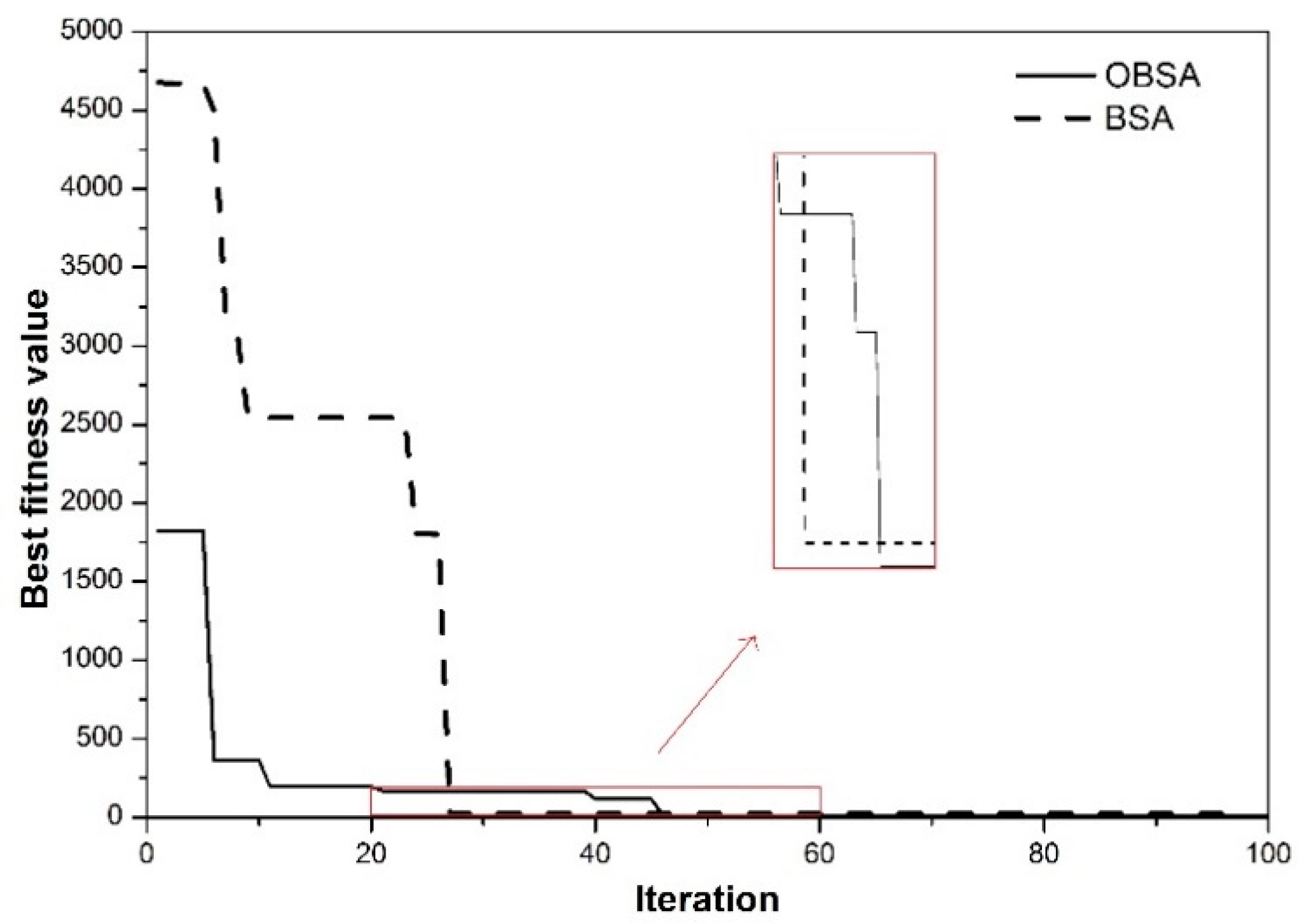
4.7. Convergence Analysis of OBSA

BSA and OBSA were used to calculate the optimal solution in this paper 20 times, and the average fitness values were calculated. The convergence curve of the average fitness is shown in Figure 12. Figure 12 shows that the convergence speed of OBSA is faster than BSA in the initial iteration and slower in the late iteration, which leads to higher convergence precision.

5. Conclusions

In this paper, with the problem of load disaggregation of using high-frequency features in non-intrusive load monitoring, a power consumption pattern-based method for low sampling data is proposed, which applied time coefficients to a traditional load disaggregation model and OBSA to optimization calculation. Experiments show that the method has a load decomposition accuracy of more than 94% for typical appliances, which can be used for the identification of similar power and normally-open appliances. The model achieved good performance in cases of multiple appliances simultaneously switching on and off.

As a load decomposition method using low-frequency features, it has better performance than the traditional mathematical optimization model using PQ features and saves computation time. Furthermore, a comparison of results with those reported in the literature proved the performance of the proposed method. Furthermore, the proposed method has better robustness at different sampling intervals, the convergence speed of the method is faster, and the convergence precision is better. The proposed method has the advantages of small hardware and software requirements for feature extraction, low sampling frequency requirements, high accuracy of load disaggregation, and suitability for use in smart grid scenarios.

Although the proposed method in this paper has the advantages mentioned above, it still has a limitation. It will misidentify the appliances whose power consumption pattern characteristic sequences are not obtained in the feature extraction stage. In order to identify unknown appliances, a feature library with as many appliances as possible can be built, but this will require a lot of work. Thus, further study will concentrate on improving the identification performance of unknown appliances.

References

1. Armel, K.C.; Gupta, A.; Shrimali, G.; Albert, A. Is disaggregation the holy grail of energy efficiency? The case of electricity. Energy Policy 2013, 52, 213–234. [Google Scholar] [CrossRef] [Green Version]
2. Grueneich, D.M. The next level of energy efficiency: The five challenges ahead. Electr. J. 2015, 28, 44–56. [Google Scholar] [CrossRef]
3. Yu, Y.; Luan, W. Smart grid and its implementations. Proc. CSEE 2009, 29, 1–8. [Google Scholar]
4. Ehrhardt-Martinez, K.; Donnelly, K.A.; Laitner, S. Advanced Metering Initiatives and Residential Feedback Programs: A Meta-Review for Household Electricity-Saving Opportunities; American Council for an Energy-Efficient Economy: Washington, DC, USA, 2010. [Google Scholar]
5. Capasso, A.; Grattieri, W.; Lamedica, R.; Prudenzi, A. A bottom-up approach to residential load modeling. IEEE Trans. Power Syst. 1994, 9, 957–964. [Google Scholar] [CrossRef]
6. Kats, G.; Capital, E. Green Building Costs and Financial Benefits; Massachusetts Technology Collaborative: Westborough, MA, USA, 2003. [Google Scholar]
7. Tabatabaei, S.M.; Dick, S.; Xu, W. Towards Non-Intrusive Load Monitoring via Multi-Label Classification. IEEE Trans. Smart Grid 2017, 8, 26–40. [Google Scholar] [CrossRef]
8. Hart, G.W. Nonintrusive appliance load monitoring. Proc. IEEE 1992, 80, 1870–1891. [Google Scholar] [CrossRef]
9. Li, R.; Wang, X.; Hu, M.; Zhou, H.; Hu, W. Application of RPROP neural network in nonintrusive load decomposition. Power Syst. Prot. Control 2016, 44, 55–61. [Google Scholar]
10. Wu, X.; Qi, B.; Han, L.; Wang, Z.; Dong, C. Fast Non-intrusive Load Identification Algorithm for Resident Load Based on Template Filtering. Autom. Electr. Power Syst. 2017, 2, 021. [Google Scholar]
11. Liu, B.; Luan, W.; Yu, Y. Dynamic time warping based non-intrusive load transient identification. Appl. Energy 2017, 195, 634–645. [Google Scholar] [CrossRef]
12. Hassan, T.; Javed, F.; Arshad, N. An Empirical Investigation of V-I Trajectory Based Load Signatures for Non-Intrusive Load Monitoring. IEEE Trans. Smart Grid 2014, 5, 870–878. [Google Scholar] [CrossRef] [Green Version]
13. Wang, A.L.; Chen, B.X.; Wang, C.G.; Hua, D.D. Non-intrusive load monitoring algorithm based on features of V–I trajectory. Electr. Power Syst. Res. 2018, 157, 134–144. [Google Scholar] [CrossRef]
14. Fernandes, R.A.S.; Silva, I.N.D.; Oleskovicz, M. Load Profile Identification Interface for Consumer Online Monitoring Purposes in Smart Grids. IEEE Trans. Ind. Inform. 2013, 9, 1507–1517. [Google Scholar] [CrossRef]
15. Aiad, M.; Peng, H.L. Non-intrusive load disaggregation with adaptive estimations of devices main power effects and two-way interactions. Energy Build. 2016, 130, 131–139. [Google Scholar] [CrossRef]
16. Cominola, A.; Giuliani, M.; Piga, D.; Castelletti, A.; Rizzoli, A.E. A Hybrid Signature-based Iterative Disaggregation algorithm for Non-Intrusive Load Monitoring. Appl. Energy 2017, 185, 331–344. [Google Scholar] [CrossRef]
17. Wang, H.; Yang, W. An Iterative Load Disaggregation Approach Based on Appliance Consumption Pattern. Appl. Sci. 2018, 8, 542. [Google Scholar] [CrossRef]
18. Yang, C.C.; Soh, C.S.; Yap, V.V. A non-intrusive appliance load monitoring for efficient energy consumption based on Naive Bayes classifier. Sustain. Comput. Inform. Syst. 2017, 14, 34–42. [Google Scholar] [CrossRef]
19. Zhou, C.; Liu, S.; Zhong, X.; Liu, P. Differential Evolution Algorithm Based Residential Load Decomposition. South. Power Syst. Technol. 2016, 10, 62–69. [Google Scholar]
20. Zhao, B.; Stankovic, L.; Stankovic, V. On a Training-Less Solution for Non-Intrusive Appliance Load Monitoring Using Graph Signal Processing. IEEE Access 2016, 4, 1784–1799. [Google Scholar] [CrossRef]
21. Makonin, S.; Ellert, B.; Bajic, I.V.; Popowich, F. Electricity, water, and natural gas consumption of a residential house in Canada from 2012 to 2014. Sci. Data 2016, 3, 160037. [Google Scholar] [CrossRef]
22. Roy, N.; Pathak, N.; Misra, A. Fine-grained appliance usage and energy monitoring through mobile and power-line sensing. Pervasive Mob. Comput. 2016, 30, 132–150. [Google Scholar] [CrossRef] [Green Version]
23. Das, S.; Suganthan, P.N. Differential evolution: A survey of the state-of-the-art. IEEE Trans. Evol. Comput. 2011, 15, 4–31. [Google Scholar] [CrossRef]
24. Jordehi, A.R.; Jasni, J. Parameter selection in particle swarm optimization: A survey. J. Exp. Theor. Artif. Intell. 2013, 259, 527–542. [Google Scholar] [CrossRef]
25. Meng, X.B.; Gao, X.Z.; Lu, L.; Liu, Y.; Zhang, H. A new bio-inspired optimisation algorithm: Bird swarm algorithm. J. Exp. Theor. Artif. Intell. 2016, 28, 673–687. [Google Scholar] [CrossRef]
26. Shi, Y.; Eberhart, R. A modified particle swarm optimizer. In Advances in Natural Computation; Springer: Berlin/Heidelberg, Germany, 1998; p. 439. [Google Scholar]
27. Mauch, L.; Barsim, K.S.; Yang, B. How well can HMM model load signals. In Proceedings of the 3rd International Workshop on Nilm, Vancouver, BC, Canada, 14–15 May 2016. [Google Scholar]
28. Batra, N.; Kelly, J.; Parson, O.; Dutta, H.; Knottenbelt, W.; Rogers, A.; Singh, A.; Srivastava, M. NILMTK: An open source toolkit for non-intrusive load monitoring. In Proceedings of the 5th International Conference on Future Energy Systems, Cambridge, UK, 11–13 June 2014; pp. 265–276. [Google Scholar]
Figure 1. Power consumption change in an operating cycle for an air conditioner.
Sustainability 11 00251 g001
Figure 2. Power consumption change curve of several typical appliances.
Sustainability 11 00251 g002
Figure 3. The algorithm implementation process.
Sustainability 11 00251 g003
Figure 4. The flow chart of OBSA solution for NILM.
Sustainability 11 00251 g004
Figure 5. Total power curve of electric furnace and refrigerator.
Sustainability 11 00251 g005
Figure 6. Disaggregation result of each appliance for example 1. The panels are listed as: (a) Disaggregation result of fridge; (b) Disaggregation result of furnace.
Sustainability 11 00251 g006
Figure 7. The total power curve of an electric furnace, air conditioner, and refrigerator are operating.
Sustainability 11 00251 g007
Figure 8. Disaggregation result of each appliance for example 2. The panels are listed as: (a) Disaggregation result of fridge; (b) Disaggregation result of furnace; (c) Disaggregation result of heat pump.
Sustainability 11 00251 g008
Figure 9. Total power curve when a clothes dryer, heat pump, electric furnace, and refrigerator are operating.
Sustainability 11 00251 g009
Figure 10. Disaggregation result of each appliance for example 2. The panels are listed as: (a) Disaggregation result of fridge; (b) Disaggregation result of furnace; (c) Disaggregation result of heat pump; (d) Disaggregation result of clothes dryer.
Sustainability 11 00251 g010
Figure 11. Disaggregation performance for the proposed model with increasing sampling interval.
Sustainability 11 00251 g011
Figure 12. Fitness values convergence curve using BSA and OBSA.
Sustainability 11 00251 g012