Article

An Integrated Modelling Approach to Study Future Water Demand Vulnerability in the Montargil Reservoir Basin, Portugal

by
Carina Almeida
1,2,*,
Tiago B. Ramos
1,
João Sobrinho
1,
Ramiro Neves
1 and
Rodrigo Proença de Oliveira
3
1
Centro de Ciência e Tecnologia do Ambiente e do Mar (MARETEC), Instituto Superior Técnico, Universidade de Lisboa, Av. Rovisco Pais, 1, 1049-001 Lisboa, Portugal
2
AQUALOGUS, Rua do Mar da China N.º 1 Escritório 2.4, Parque das Nações, 1990-137 Lisboa, Portugal
3
Civil Engineering Research and Innovation for Sustainability (CERIS), Instituto Superior Técnico; Av. Rovisco Pais, 1, 1049-001 Lisboa, Portugal
*
Author to whom correspondence should be addressed.
Sustainability 2019, 11(1), 206; https://doi.org/10.3390/su11010206
Submission received: 13 November 2018 / Revised: 21 December 2018 / Accepted: 26 December 2018 / Published: 3 January 2019

Abstract

:
This paper describes an integrated modelling approach to study water use vulnerability in a typical Mediterranean basin under different climate change projections. The soil water assessment tool (SWAT) and the MOHID (from modelo hidrodinâmico) Water model were used to evaluate the impacts of two climate scenarios (GFDL-ESM2M and IPSL-CM5A-LR) on water availability in Montargil’s basin and reservoir (Portugal) during two decadal timelines (2030 and 2060). Reservoir performance metrics were estimated considering also two water demand scenarios: an average of the water demand in the last 10 years; and the largest annual demand of the last 10 years. The SWAT model results showed a future decrease of inflows to the reservoir, with its volumetric reliability decreasing from 100% in the historical simulation to about 60–70% in the IPSL-CM5A-LR climate scenario and 40–50% in the GFDL-ESM2M climate scenario. The time reliability also decreased to less than 30%, while the resiliency for the water demand decreased to an average 20–35% for both climate scenarios. These impacts indicate the importance of the managing systems in an integrative mode to prevent water resources reduction in the region.

1. Introduction

In the Mediterranean region, water resources are scarce and exhibit large seasonal and intra-annual variability. Water storage is essential for fulfilling water demand, for producing energy and for controlling flood and drought events. The sustainability and development of many economic activities in the region depends on water storage in reservoirs, with the construction of infrastructures in river valleys also leading to changes in land use that influence the entire water balance and water quality at the basin scale.
Basins are subjected to multiple stressors [1,2,3], with climate change emerging as a major concern in river water management. In the Mediterranean countries, surface air temperature is expected to increase while the annual amount of precipitation is expected to decrease [4,5,6,7]. These changes will result in an increasing frequency of extreme climatic events, including droughts [8,9]. Examples of these extreme events are already visible in Portugal, where severe drought events occurred during 2005 and 2012 [10]. As a result, surface and ground water availability is projected to decrease, especially in the centre and south of Portugal [11], stressing the need for developing strategies for adapting water resources management to climate change.
In southern Portugal, several reservoirs were built in the middle of the 20th century, mainly for irrigation. New irrigated areas were created, with crops having their growing season in the summer season when evapotranspiration needs are higher [12]. This production system is highly dependent on water stored in reservoirs during the rainy season and on the existence of hydraulic structures to distribute water.
In the past, infrastructure planning and operations, namely reservoir water management, was based on the analysis of historical records, which were assumed to be stationary. In the context of climate change that may not be the most appropriate strategy. Instead, a growing number of studies have pointed to the importance of integrating mathematical models in the decision-making process [13,14,15]. Mathematical models can provide managers with an integrative analysis of the processes and time variables concerning the basin status [16,17], which otherwise would be difficult to assess only with available monitoring results. Models can also provide, directly or indirectly, performance indicators related to water resource use that can be used to evaluate its operating rules, determining the supply guarantee, the vulnerability of water needs, and the system’s resilience [18,19].
By considering climate change and related uncertainty, those modelling tools can be used for predicting water availability in the near future. This results in a direct benefit when estimating inflows or planning of best operation practices, particularly in basins where agriculture is heavily dependent of reservoirs supply. Additionally, while most of the uncertainty associated to long-term hydrological predictions refers to the ability of climate model to forecast future precipitation for the river basin, climate models have been consistent in the projected trends allowing to draw reliable future scenarios.
The complexity of the dynamics and properties of each water body such as lakes, rivers or coastal areas, or even artificial systems such as reservoir or urban systems further require the integration of mathematical models for improving water resources management. Thus, extensive integration of mathematical models has been performed during the last decades. For example, Brito et al. [15] integrated the basin (soil and water assessment tool (SWAT) model) and reservoir model (CE-QUAL-W2) to study the water quality and to test different management scenarios to reduce nutrient loads in an eutrophic reservoir in southeast Portugal. Brito et al. [20] developed an operation management tool for simulating flows from the main watersheds of the Iberia Peninsula, where the basin model MOHID Land (from modelo hidrodinâmico) were intergrated in the coastal model MOHID Water.
In this study, two climate models were used as input to a basin model, which in turn was integrated into a reservoir model. The main objective was to investigate water resources availability in the Montargil reservoir (southern Portugal) and respective vulnerability under future climate scenarios. The specific objectives were: (1) to assess and model climate change scenarios over the study area; (2) to determine the water balance and flows at the basin scale; and (3) to analyse the vulnerability of the reservoir while considering those future scenarios. This study is particularly original in performing an integrated analysis of water resources availability in the Mediterranean region under the context of climate change. This study further promotes the development of tools to support sustainable water resources management in the study area.

2. Materials and Methods
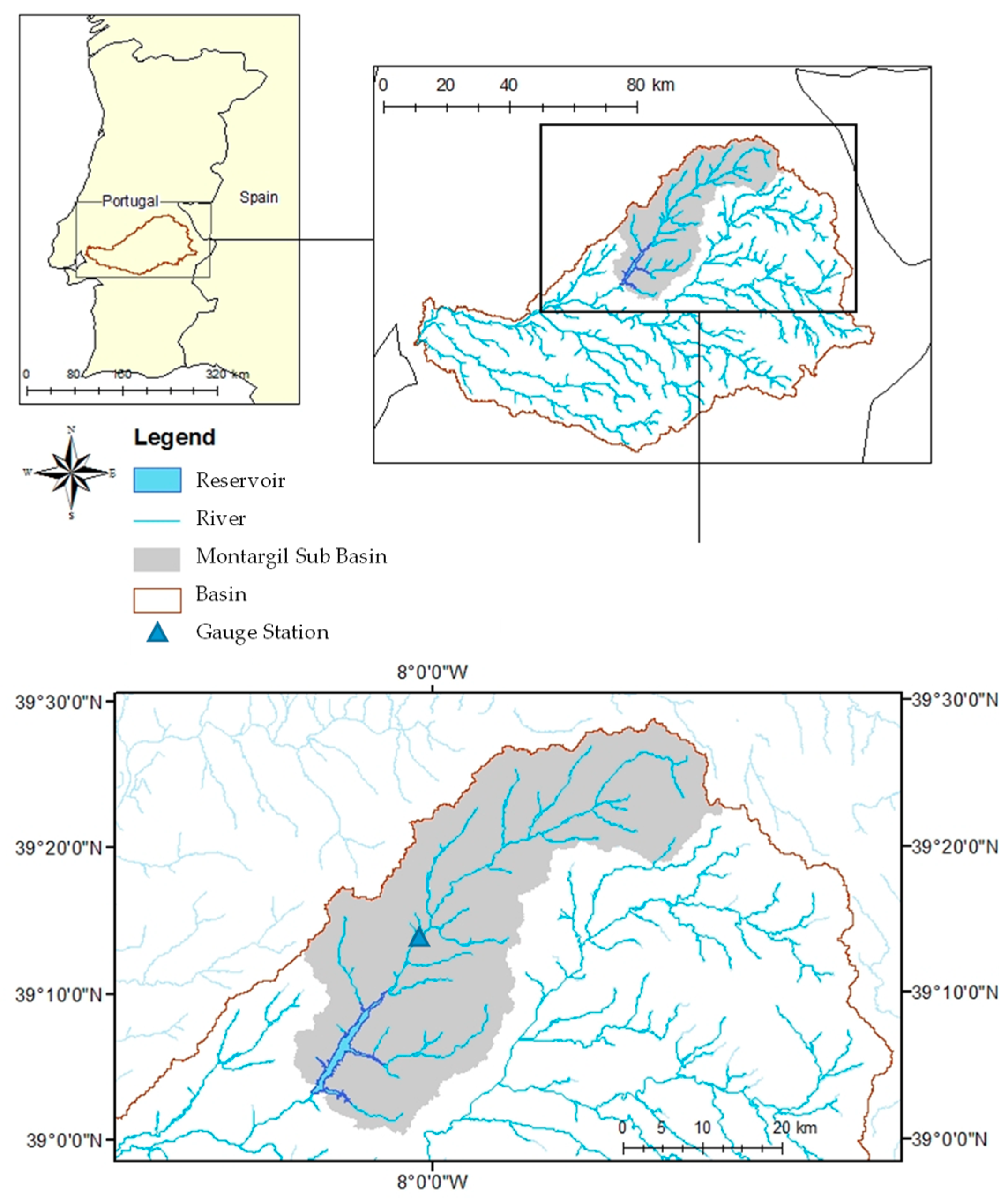
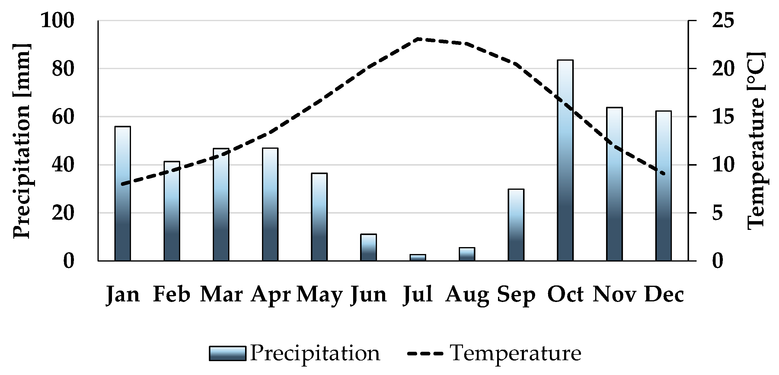
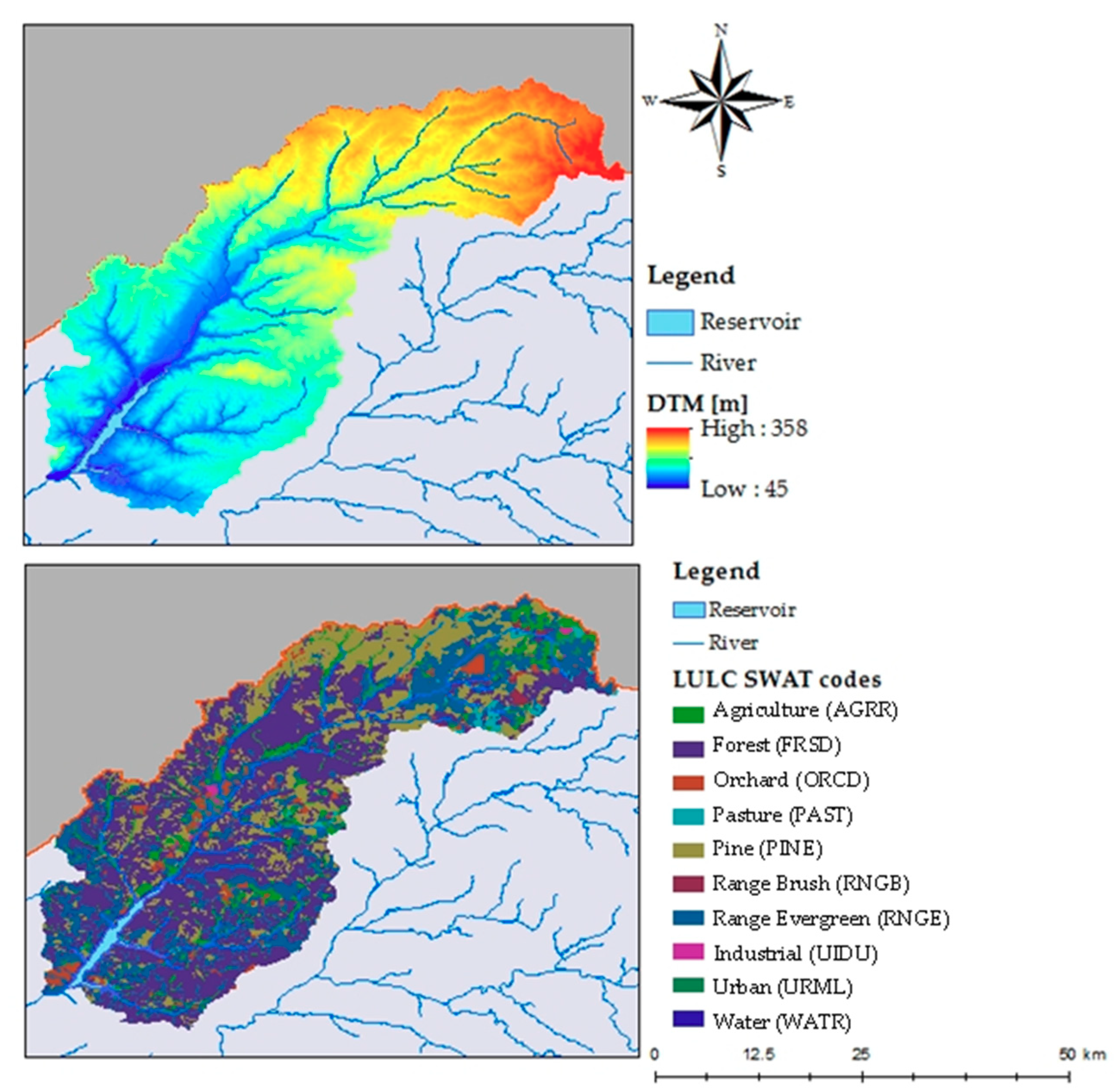
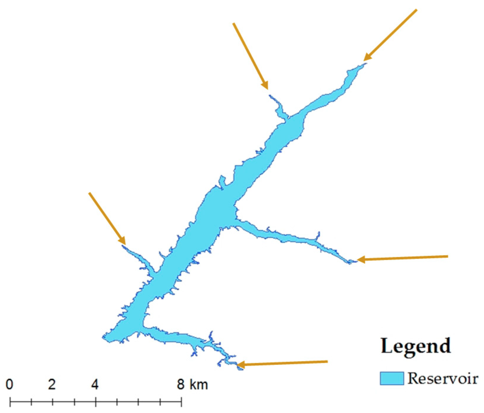
2.1. Study Area

This study was carried out in the Montargil Reservoir, located in the Sôr River sub basin, which is part of the Sorraia River (southern Portugal), the tributary of the Tagus River with the largest basin area (~7730 km2) (Figure 1). Montargil, with its drainage area of ~1200 km2, is one of the largest Portuguese reservoirs on a dry area. This reservoir is part of the Sorraia Valley watering system with two other reservoirs: Magos and Maranhão. The system was created between 1951 and 1959 and benefits a total of 16,351 ha of irrigated agricultural land in six municipalities. The watering system is managed by the Farmers Association of the Sorraia Valley (ARBVS) since 1970. Thus, while each reservoir has an independent drainage area, they are managed together according to water availability.
Over the last years, the Montargil reservoir has been increasingly used for recreational purposes, benefiting from short distances to major urban habitation areas (about 100 km from Lisbon) and warm water temperatures during the bathing season. The reservoir has also been used for electric power generation, fishing, and water sports. The climate in the region shows two typical seasons, one with dry and hot summers, and another with mild and wet winters (Figure 2).
The main land uses in the Montargil basin area are forest (63%), range-grass (22%), agriculture (8%), orchard (3%), urban and industrial (1%) and pasture (1%) [21] (Figure 3). The elevation ranges from 45 to 358 m a.s.l (Figure 3). The dominant soil types are Cambisols, Luvisols and Regosols [22].
The Montargil reservoir provides mainly water for irrigation, and to a less extent for industry purpose. The water level is thus regulated by irrigation water demand and depends on climatic conditions. Accordingly, the reservoir is filled between autumn and spring and the water is used gradually during the summer irrigation season (Figure 4). The outflow from the reservoir is controlled by several structures. The maximum reservoir capacity is about 164 hm3, with a water surface elevation of 80 m and minimum surface height of 30 m. The minimum water surface elevation acceptable for operation is 65 m above water surface elevation, which corresponds to ~143 hm3.

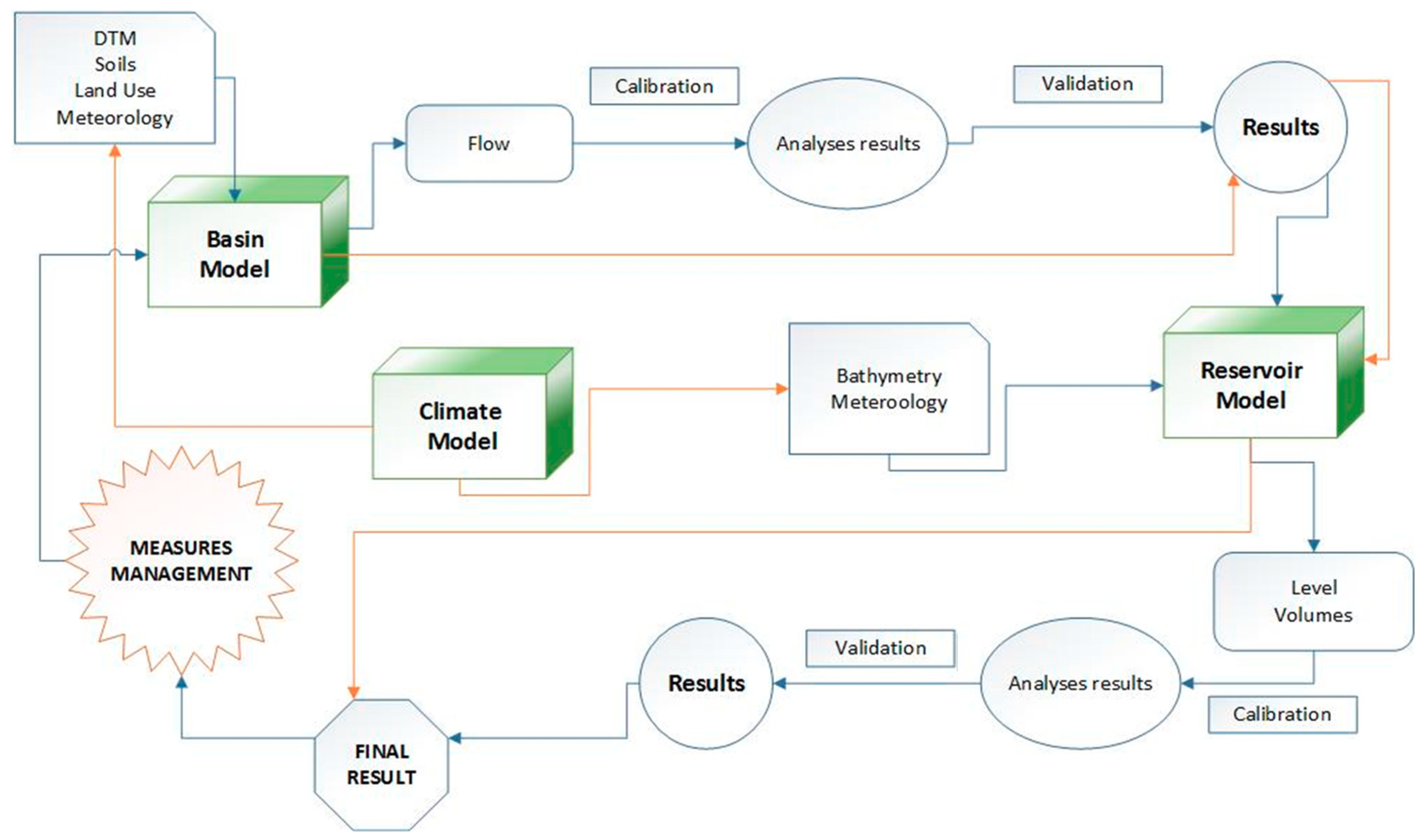
2.2. Integrated Modelling Approach

Figure 5 describes the framework of the integrated modelling approach considered in this study. The SWAT [23] was used for modelling flows at the basin scale. The basin modelling considered the digital terrain model (DTM), soil data, land use, and meteorology from historical data as inputs. The model was calibrated and validated by comparing simulated flows with measured data. The baseline simulation was defined for the period between 1996 and 2015. The SWAT model was calibrated manually for the period between 2001 and 2006, while the validation exercise comprised the period from 2006 to 2015. Flow results from SWAT were then integrated as boundary conditions to the reservoir MOHID Water model [24]. This model was calibrated and validated for simulating the elevation-volume curve, levels, and volumes during the historical period (Figure 5). After model validation, future scenarios were defined using projections from the GFDL-ESM2M and IPSL-CM5A-LR climate models [25,26] as boundary conditions to SWAT and MOHD Water. The description of each model can be found in the sections below.

2.2.1. Basin Model

The SWAT [23] is a semi-distributed widely used model for simulating watershed processes and assessing land management practices at the basin scale using a daily time step. The SWAT model was already successfully calibrated/validated for simulating streamflow and nutrient dynamics in the Sorraia basin [3,27], with results providing the necessary basis for conducting this study. The model splits the watershed into sub-basins that are assumed to be homogeneous in their hydrologic response units (HRU), i.e., areas with homogeneous properties in terms of slope, land use, and soil type. The hydrology of the model relies on solving the water balance equation, as follows:
SW t = SW 0 + i = 1 t ( R day Q surf E a W seep Q gw )
where SWt is the final soil water content (mm), SW0 is the soil water content at the initial time step (mm), Rday is the precipitation on day i (mm), Qsurf is the surface runoff on day i (mm), Ea is the actual evapotranspiration on day i (mm), Wseep is the percolated water on day i (mm), and Qgw is the return flow on day i (mm).
Crop evapotranspiration is computed following the Penman Monteith method [28], and dependent on soil water availability. Infiltration and groundwater flow are computed based on empiric or semi-empiric formulations (as the Soil Conservation Service (SCS) rainfall-runoff curves or soil-shallow aquifer-river transfer times). Details on individual simulation components can be found in Neitsch et al. [23].
In this study, the SWAT model was applied to the Montargil sub-basin using the ArcGIS extension from ESRI (Redlands, CA, USA). Available geographic information system (GIS) maps of topography from Shuttle Radar Topography Mission (SRTM) with 90 m resolution, land use from GSE Land M2.1 with 20 and 300 m resolution [21], and soils from Portuguese Soil maps and Land use Capacity at 1:25,000 scale [29], were used. Climatic maps, including daily precipitation, temperature, relative humidity and wind speed were derived from the Portuguese National Institute of Water Resources (SNIRH) [30].

2.2.2. Reservoir Modelling

The present work was carried out using the hydrodynamic and biogeochemical three-dimensional MOHID Water model [24]. This model has been applied to a variety of locations subject to different conditions since its creation [31,32,33]. The model consists of a set of modules interconnected using an object-oriented programming. Each module is responsible for the management of part of information, constituting a total of 40 modules developed over 3 decades of research work.
In this study, the MOHID Water model was applied to the Montargil reservoir. The following modules were considered for simulating water variation dynamics in this study: Atmosphere, Geometry, Hydrodynamic, Interface Water Air, Turbulence and Discharges. The model grid resolution was 100 m × 100 m, and the topography map from the SRTM with 90 m resolution was considered due to unavailability of the bathymetric map of the Montargil reservoir. As initial condition, the water level at the first day of the simulation was imposed from SNIRH [34]. Meteorological data (velocity and wind direction, precipitation, solar radiation, air temperature and relative humidity) were obtained from SNIRH [34] and used as boundary conditions. The upstream river discharges computed earlier with the SWAT model were also used as boundary conditions. These were set to reach the reservoir on five locations (Figure 6), with the main river inflow reaching ~48 m3/s (average of 10 years), while the four lateral smaller tributaries reached ~19 m3/s. Finally, the effluent reservoir discharge provided from ARBVS was considered as outflow, translating the water used for irritation purposes in the downstream area.

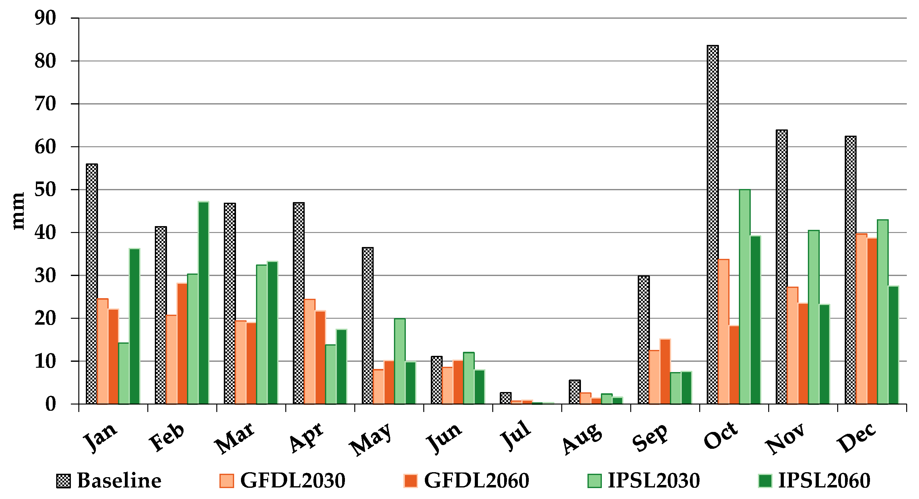
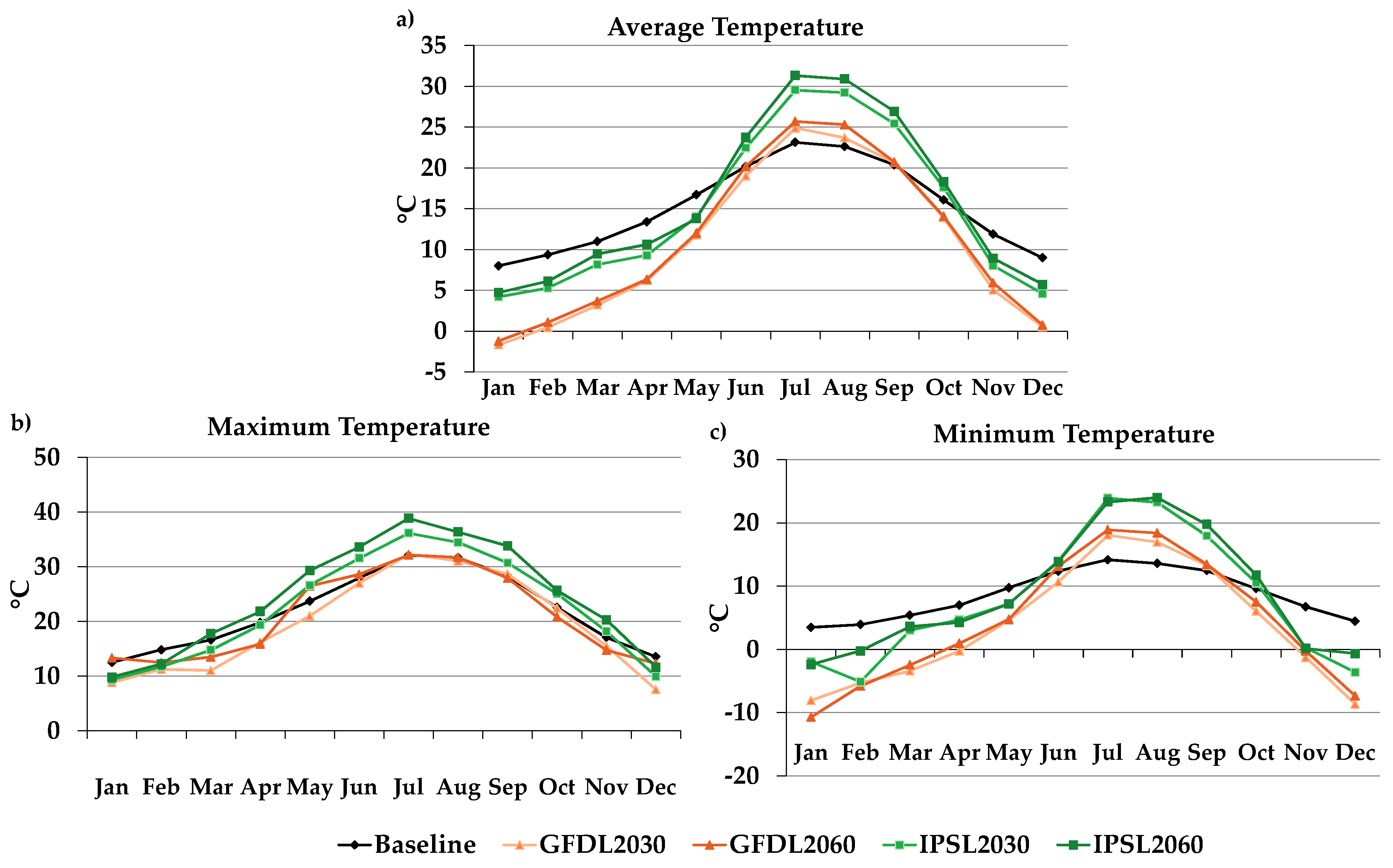
2.2.3. Climate Models

The climate models adopted in this study were the GFDL-ESM2M [25] and IPSL-CM5A-LR [26]. These models followed the framework established by Sanchez et al. [34] and Birk et al. [35] during the Project “Managing Aquatic Ecosystems and Water Resources Under Multiple Stress—MARS” [3,36], where this work is embedded. In the MARS Project, three societal scenarios were developed and implemented in the Sorraia basin [27], based mainly on agriculture practices and on the work of O’Neill et al. [37] and Riahi et al. [38]. These authors defined Shared Socioeconomic Pathways (SSPs) as reference scenarios describing plausible alternative trends in the evolution of the society and ecosystems over a century timescale in the absence of climate change or climate policies. The surface air temperature and precipitation time-series were downscaled at a 0.5° resolution according to the The Inter-Sectoral Impact Model Intercomparison Project (ISI-MIP) project [39,40]. Differences between the GFDL and IPSL models and downscaling of variables at the basin-scale acquired from the outputs of these two models are given in Warsawski et al. [39] and references therein.
For the case of Montargil sub basin, this study took into consideration the storyline based on the combination of the Shared Socioeconomic Pathway-2 (SSP-2) defined as an intermediate stage in the evolution of the society and ecosystems over a century timescale [38,39], and the Representative Concentration Pathways 4.5 (RCP 4.5). According to Moss et al. [41], the RCP 4.5 assumes a greenhouse gas emission with peak around 2040 followed by a decline.
Additional bias-correction for the study area was carried out in Almeida et al. [27] and considered the temperature and precipitation historical data for the period between 2006 and 2015. The period from the last 20 years (1996–2015) was selected as a reference for the present condition (baseline simulation) and the two distinct temporal intervals were set up to run the future simulations: 2030 (defined as a 10-years average from 2025 to 2034) and 2060 (defined as a 10-years average from 2055 to 2064).
Both climate models show a decrease of precipitation when compared to the historical data from 1996 to 2015, here considered as the baseline condition (Figure 7), with the monthly average decreasing from ~22 to ~9 mm during the Spring/Summer season. Similar behaviour is observed during the Autumn/Winter season, with the GFDL model estimating monthly average decreases from ~59 mm to ~28 mm and ~25 mm for the 2030 and 2060 timelines, while the IPSL model shows a decrease to ~35 mm and ~34 mm during the same timelines. Concerning temperature, predictions showed fluctuations of monthly values, with more extreme maximum and minimum values being noticed (Figure 8).

2.3. Performance Indicators

Several performance indicators were adopted to evaluate the system reliability, resiliency, and vulnerability based on monthly failure events registered in the Montargil reservoir. The reliability is the oldest and widely used indicator for assessing water resources systems performance. This was defined by Hashimoto et al. [18] as how often the system fails:
Reliability = P{S ∈ NF}
where P is the probability, S is the system state variable under consideration and NF is related to the non-failure state. The most recognized and applied definition uses the concept of failure which occurs when the system is unable to satisfy water needs. The time reliability can be estimated as:
Reliability = 1 - j = 1 M d ( j ) T
where d(j) is the duration of the failure event j, M is the number of failure events, and T is the total number of time intervals. The volumetric reliability is defined as the percentage of needs during the simulation period that were satisfied.
Resilience is defined as the measure how quickly the system returns to a satisfactory state once a failure has occurred. The resiliency provides an indication of the system’s capability to recover from a failure. Hashimoto et al. [18] define resilience as a conditional probability:
Resilience = P{S(t +1) ∈ NF | S(t) ∈ F}
where S(t) is the system state variable. This definition of resilience is equal to the inverse of the mean value of the time the system spends in an unsatisfactory state, i.e.,
Resilience = { 1 M j = 1 M d ( j ) } - 1
where d(j) is the duration of the failure event j and M is the total number of failure events.
Vulnerability indicators are used to assess the severity of failure when it occurs and was defined by Hashimoto et al. [18] as:
Vulnerability = j = F e ( j ) . h ( j )
where h(j) is the most severe outcome of the failure event j and e(j) is the probability of h(j) being the most severe outcome of a failure resulting into unsatisfactory state. Hashimoto et al. [18] and Jinno et al. [19] estimated posteriorly vulnerability as the mean value of the deficit events v(j) as:
Vulnerability = 1 M j = 1 M v ( f )

3. Results and Discussion

3.1. Basin Modelling

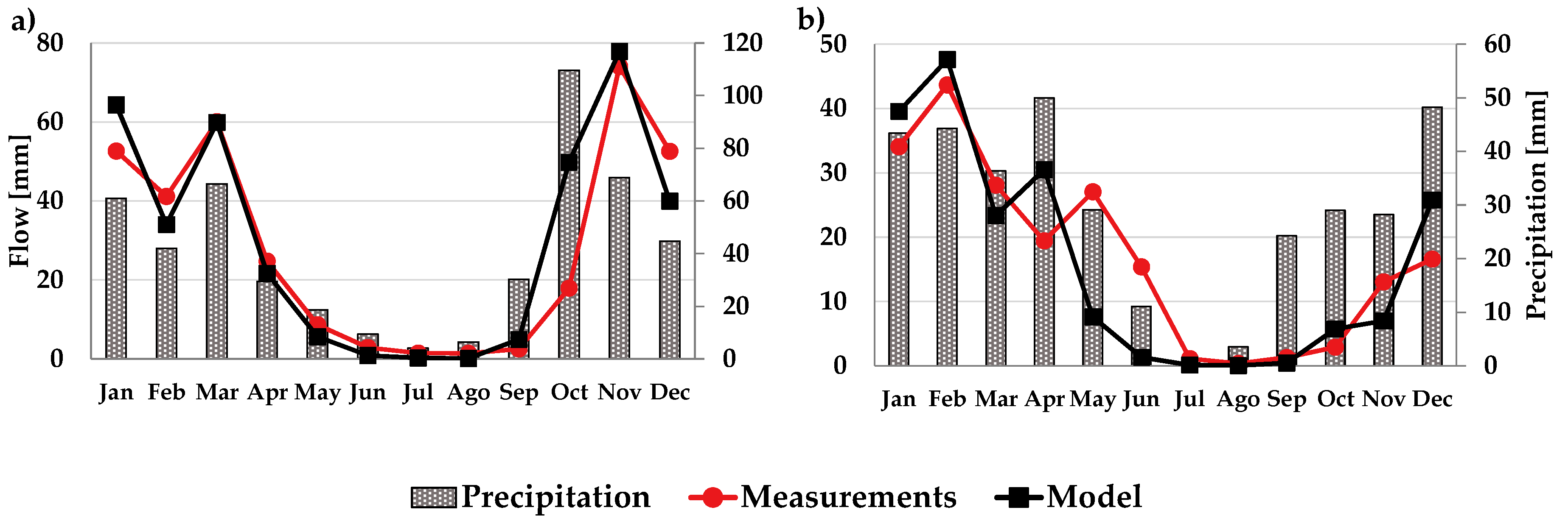
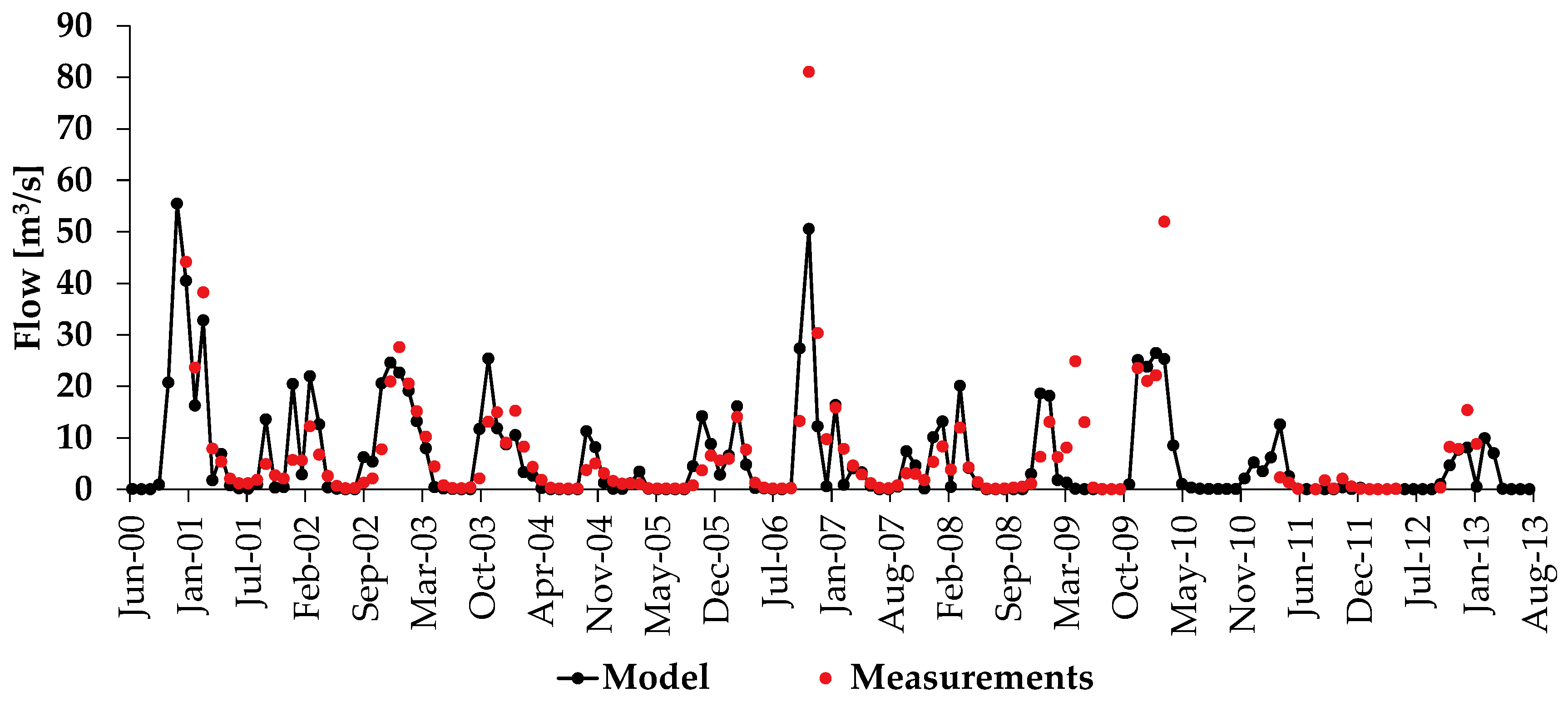
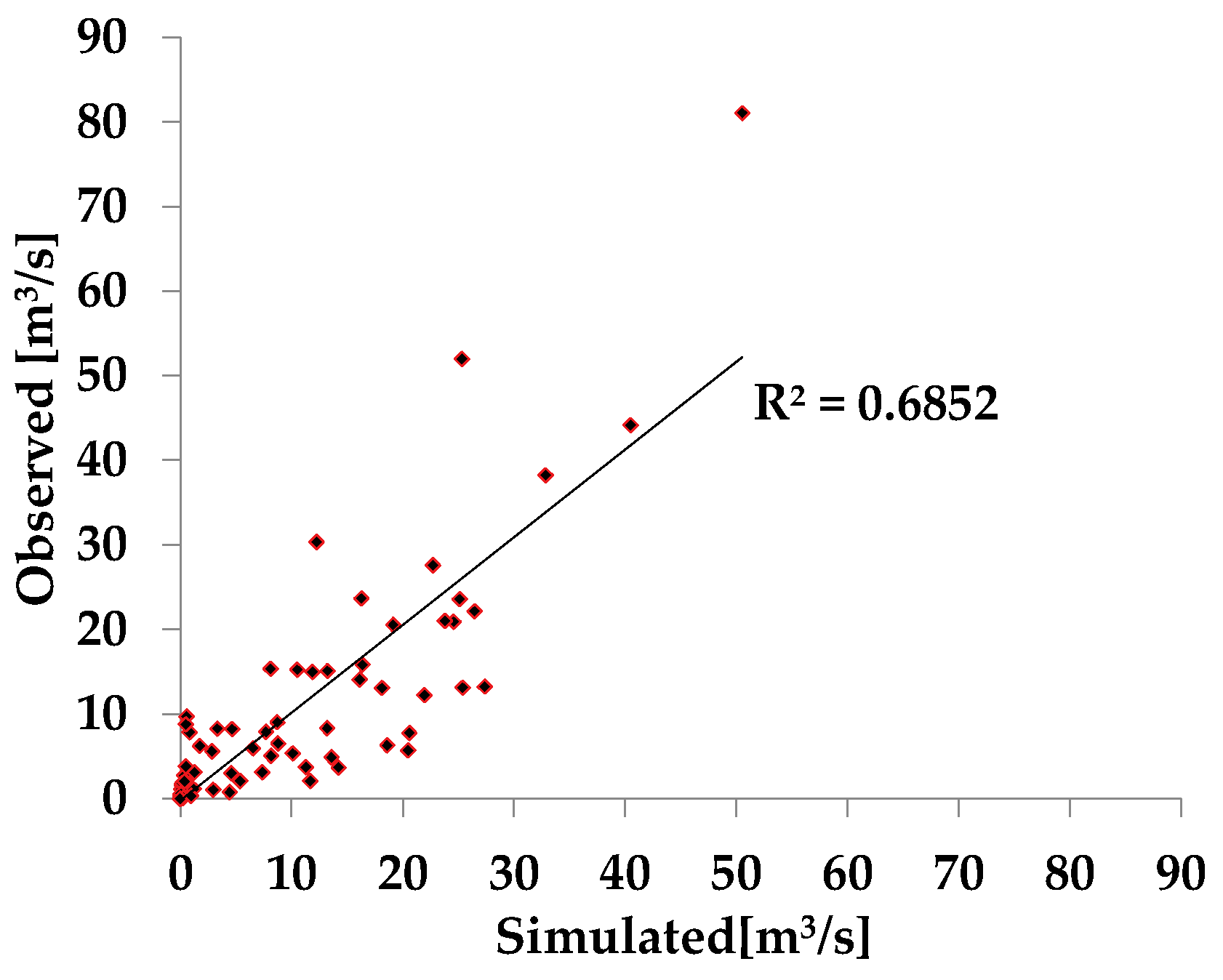
3.1.1. Calibration and Validation

The SWAT model calibration and validation for the Montargil sub basin was carried out by comparing simulated and observed flows at the Moinho Novo hydrometric station (Lat. 39.228°; Long. −8.029°). The SWAT parameters CN2, ALPHA_BF, GW_Delay, SOL_AWC, SOL_ZMX, SOL_Z1 and SOL_Z2 (Table 1) were thus modified until deviations between simulated and observed data were minimized.
The statistical indicators obtained after comparing the monthly simulated and measured flow values at the Moinho Novo monitoring station were: the coefficient of determination (R2) of 0.71, the root mean square error (RMSE) value of 6 m3/month, and the Nash–Sutcliffe efficiency (NSE) value of 0.71. The R2 showed that a considerable proportion of variability of the observed data was explained by the model. The RMSE indicated a small error of model estimates. The NSE indicates that the residual variance resulted much smaller than the measured data variance (Figure 9 and Figure 10). For the validation period, the indicators were found to be similar, indicating a reasonable calibration of model parameters when considering all uncertainties related to measurements (Figure 9 and Figure 10). Similar performances of the SWAT model can be found in other watersheds of the same size in the Mediterranean region. For example, Briak et al. [42] simulated streamflow in the Kalaya watershed, northern Morocco, obtaining a NSE value of 0.76. Bucak et al. [43] did the same for the watersheds of Lake Beyşehir, Turkey, producing R2 values from 0.38 to 0.78 and NSE values from 0.37 to 0.76. Also, Dechmi et al. [44] obtained high R2 and NSE values of 0.90 in the Del Reguero River watershed in northern Spain, while Panagopoulos et al. [45] found R2 values of 0.86–092 and NSE values of 0.51–0.68 in the Arachtos catchment, in western Greece. The SWAT model performance in the study area was particularly good (R2 = 0.685) during the rainy period (autumn and winter season) when flows were higher (Figure 11), which is particularly relevant due to the importance of the high flow season for reservoir management.

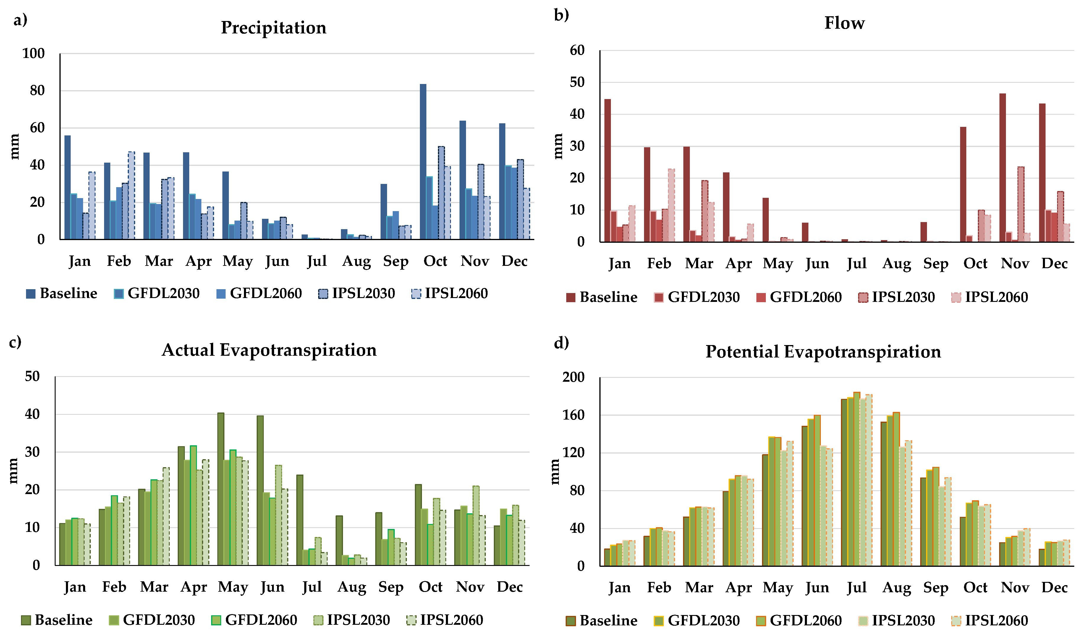
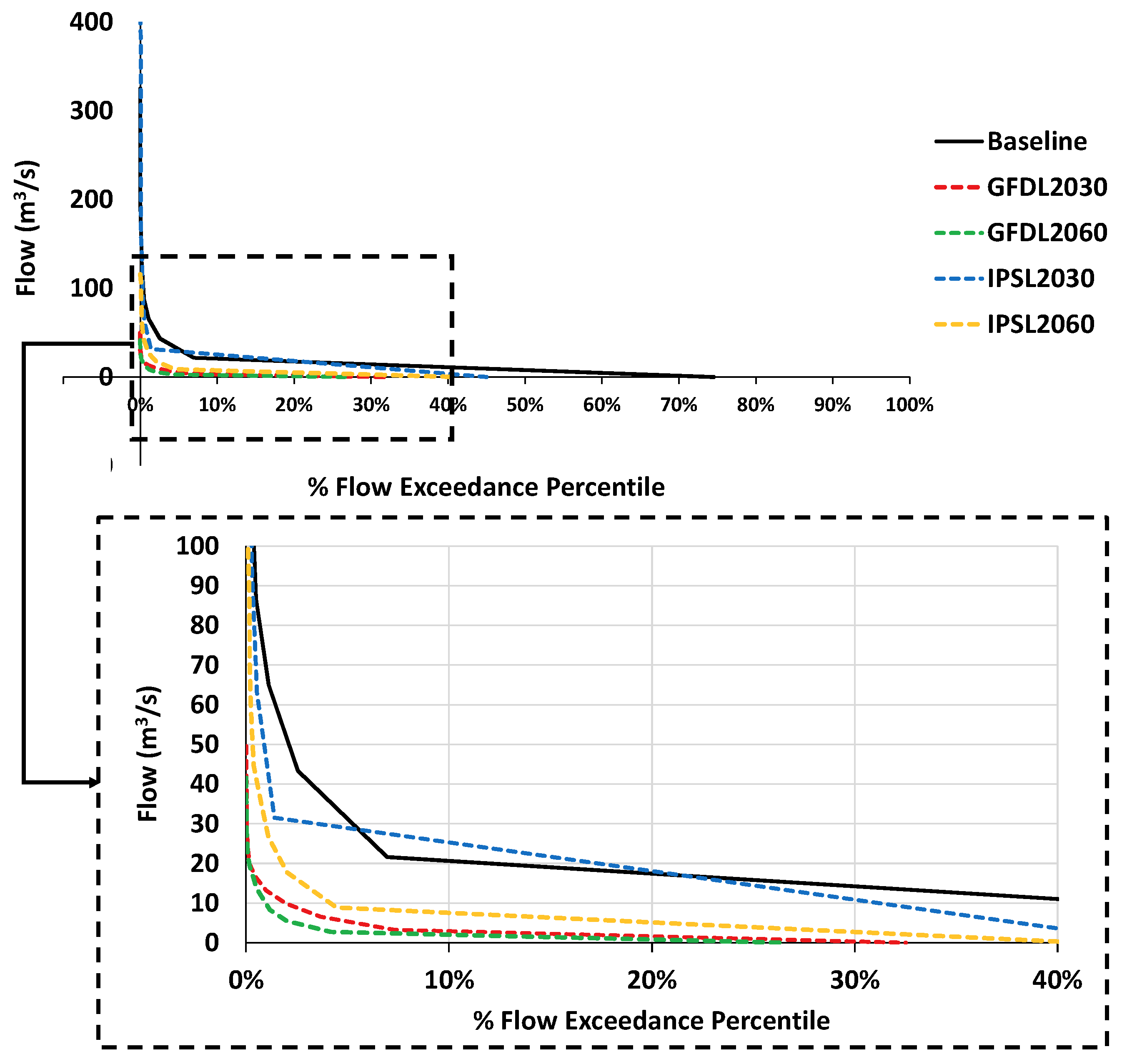
3.1.2. Water Availability

After calibration and validation, the SWAT model was used to determine the long-term water balance of the Montargil catchment for different scenarios. The monthly water balance considers precipitation, flows and actual evapotranspiration. The results indicate two distinct seasons. During autumn and winter, i.e., from October to March, precipitation and flows are high. Conversely, during spring and summer, between April and September, precipitation and flows are low (Figure 12).
The expected precipitation reduction for all scenarios leads to a decrease of monthly flows (Figure 12), in line with previous studies [27,39,40,46,47]. Higher temperatures, which result in an increase of potential evapotranspiration, also concur with this situation (Figure 12). The baseline monthly actual evapotranspiration values are in accordance with the detailed work developed by Simionesei et al. [48] to pasture and Ramos et al. [49] to maize grown in the Sorraia basin. Vegetation growth in the region may be compromised due to higher water stress as a result of higher evapotranspiration demand and limitations in water available for irrigation.
The flow duration curves (Figure 13) show a decrease of flows with exceedance values Q95% from 1.7 m3/s in the baseline scenario to values of approximately 0 m3/s (Figure 13). The single exception is the IPSL climate model for the 2030 timeline scenario, which maintains some low flows with a Q95% (~1.2 m3/s) close to the baseline value (~1.7 m3/s). The two climate models differ when projecting high flows events. The GFDL model projects a decrease of Q10% from 20 m3/s to ~2.5 m3/s and 2.8 m3/s for the 2030 and 2060 timelines, respectively. In an opposite way, the IPSL climate model suggests a similar value of the Q10% value to 18 m3/s for the 2030 timeline and increase to 25 m3/s for 2060. This may be due to the increase of predicted high precipitation events that resulted in flow peaks as showed already in several studies in Mediterranean region [7,9,27] and especially in Almeida et al. [27] for the Sorraia basin, whose results show the impact of precipitation to water availability in the basin. Those results we mainly related to climate change projection and management practices, which are expected to affect directly the reservoir water availability and consequently its vulnerability, especially during the irrigation season when a higher water demand is expected.

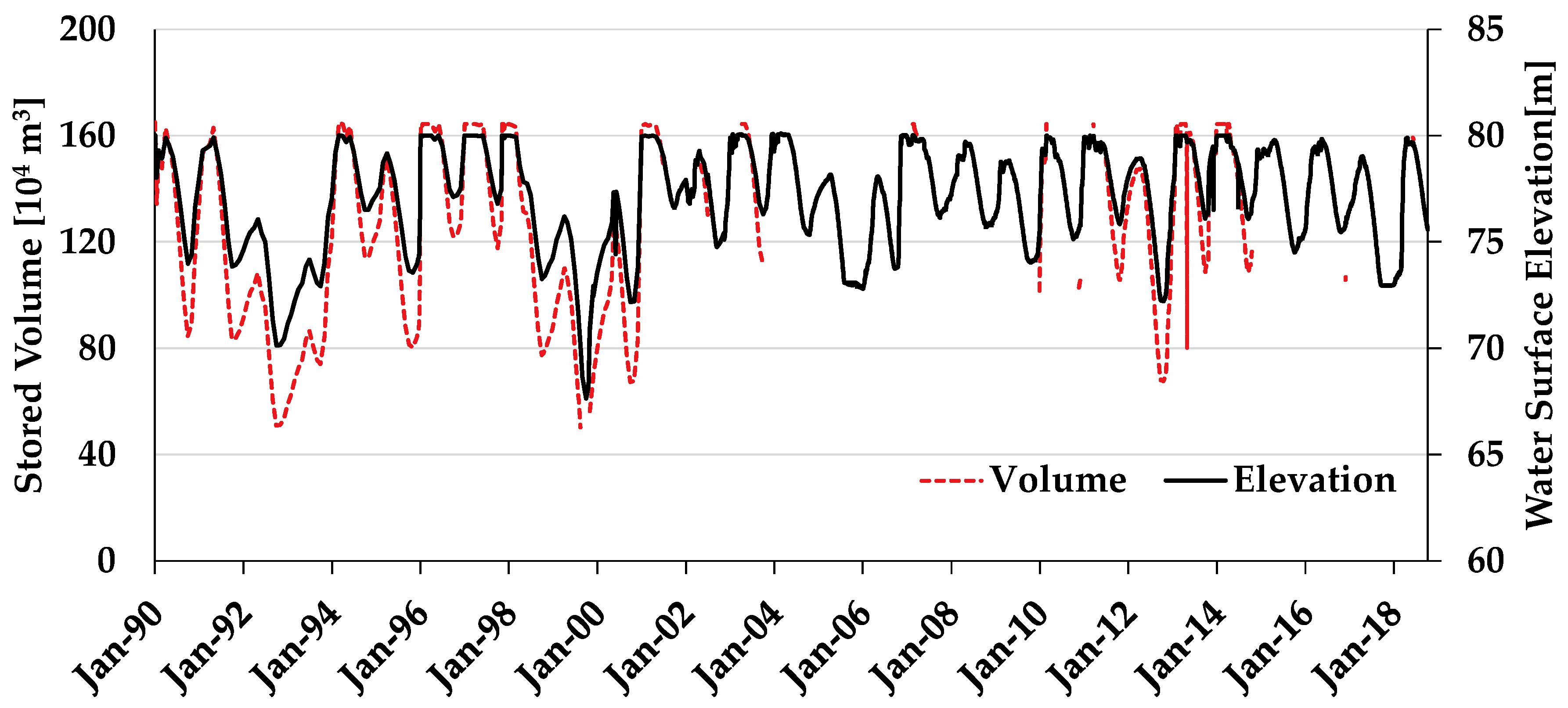
3.2. Reservoir Modelling
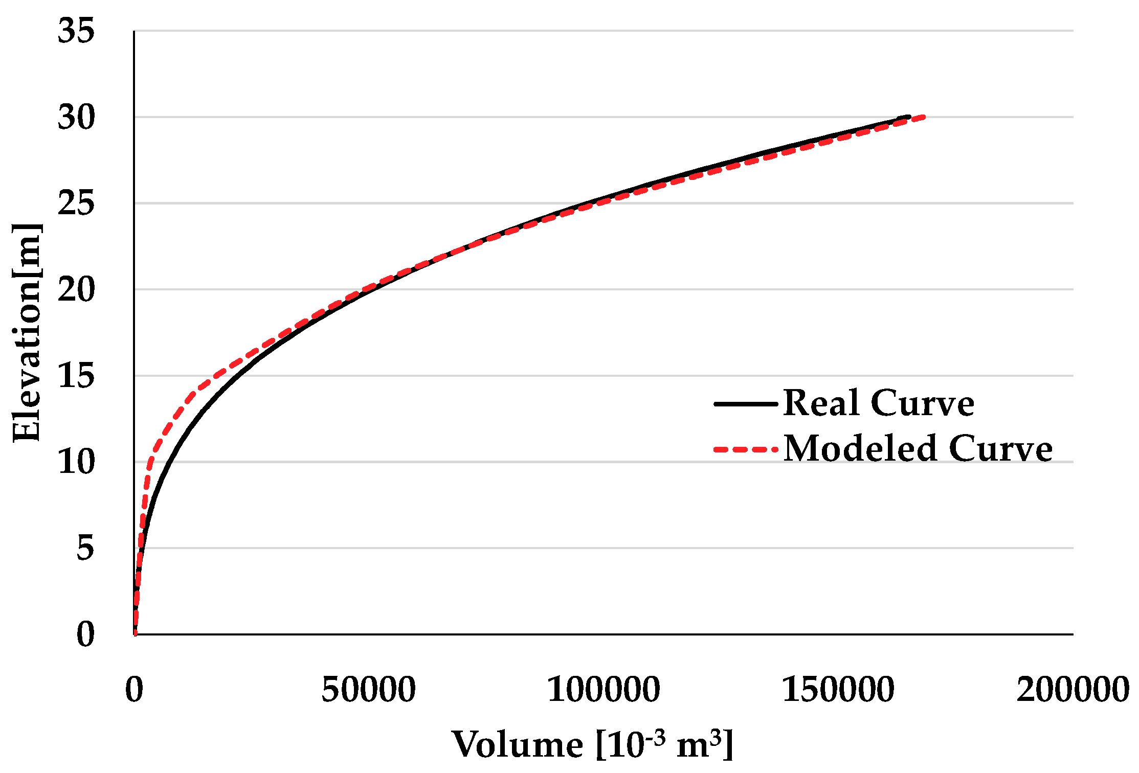
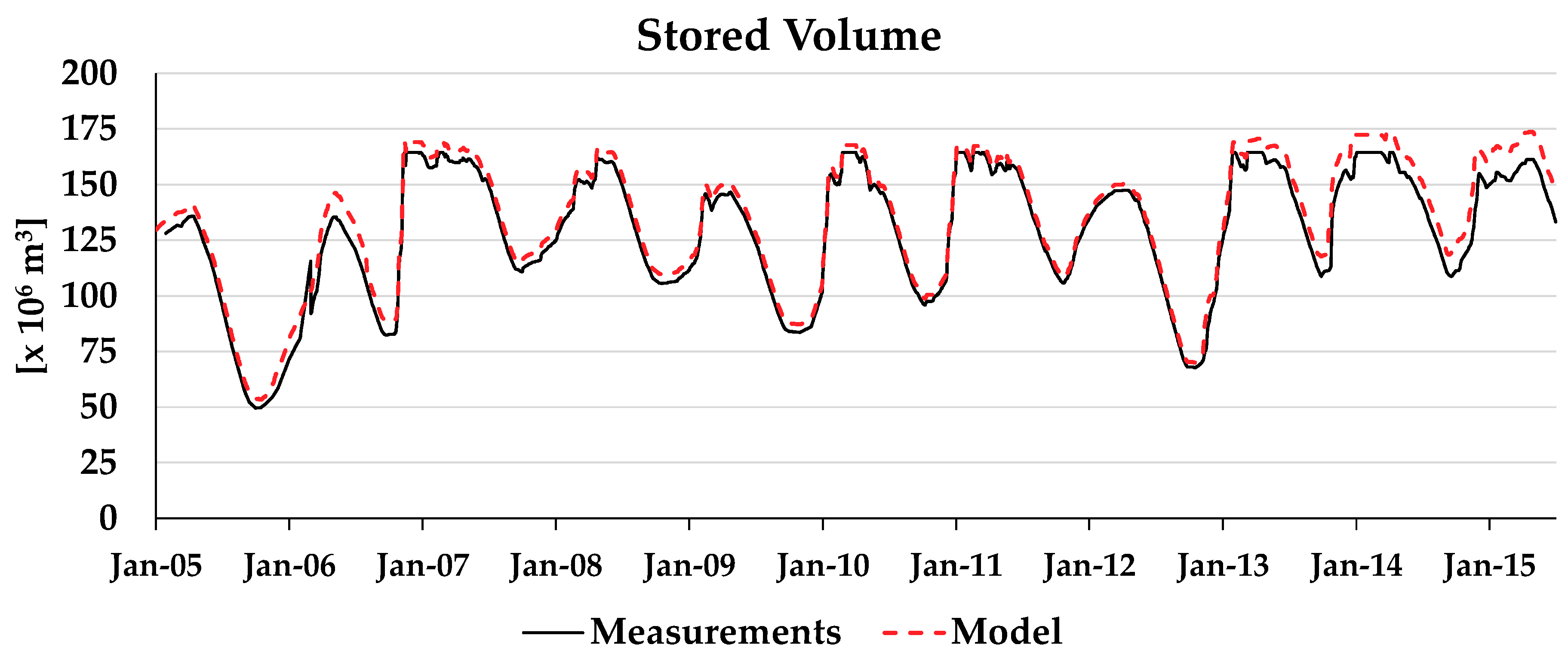
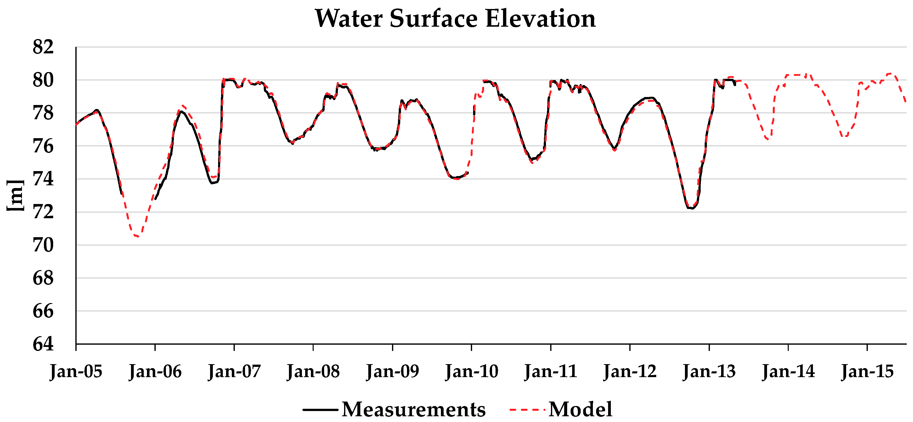
3.2.1. Validation

The SWAT flow estimations presented above were introduced as boundary conditions to the MOHID Water reservoir model. The baseline for simulating reservoir operation was defined from 2005 to 2014. A topography map with 90 m resolution was converted and adjusted into the 100 m resolution grid considered in the MOHID Water model using the tools available in MOHID Studio. Figure 14 compares the elevation–volume curve considered in the model with the one obtained from measured data. The simulation of the baseline period shows a close match between the computed and observed water surface elevation and stored volume values (Figure 15 and Figure 16). The R2 value obtained for the stored volumes is 0.987 while for water levels is 0.988. These results are in accordance with Brito et al. [15], who applied a similar model to study the Enxoé Reservoir dynamics in southern Portugal. Similar good results were obtained by Lee et al. [50] for the Hodges Reservoir, San Diego, USA, and Noori et al. [51] for the Karkheh Reservoir, Iran, using the same model.

3.2.2. Water Availability

After validation of the MOHID Water model, results were analysed on a monthly basis to understand the future behaviour of the Montargil reservoir and assess the impact of flow reduction on the reservoir ability to meet agriculture water demand. At this stage, two demand scenarios were considered by modifying the reservoir output discharge imposed in the MOHID Water model:
-
Assuming the average water demand in the past 10 years;
-
Considering the year with maximum water demand in the past 10 years, which correspond to a water demand increase of ~30% when compared with the average year. The second water demand scenario reflects the increase of irrigation in the Sorraia basin since water is mainly used for this purpose.
To better understand the performance of the reservoir and its operating rules under climate change, the indicators described above were considered to determine the supply reliability, vulnerability of water needs, and the system’s resilience for each simulated scenario. This approach has been applied in several reservoir studies, including the Sorraia basin where the Montargil reservoir is included [52,53,54]. As a failure reference, the volume of ~10 hm3 was considered in case of extreme necessity when half of the dead volume could be used.
The first water demand scenario (the average water demand in the past 10 years) resulted in an increase of monthly failures for both simulated climate scenarios and timelines (Figure 17 and Table 2). This shows that in the future, the stored volume is expected to be below the dead volume for several months, something that has never happened in the past (Figure 15). This is mainly due to the impact of runoff decrease in the reservoir, which is consistent with the literature as shown by Mateus et al. [54] when studying the reliability of six reservoirs in Scotland or Afzal et al. [55] when analyzing the vulnerability of the Pong reservoir, India. Future water demand scenarios considered in both studies showed a reliability reduction and a vulnerability increase of the simulated reservoirs, advancing then with future water management strategies to cope with those predictions. The same was considered by Fiering et al. [56], proposing also mitigation strategies when vulnerability increases above 25%.
The volumetric reliability, i.e., the percentage of needs that are satisfied during the simulation period, is higher when the IPSL climate model predictions are considered, reaching about 73% in both timelines (Table 2). The annual reliability is only 30% and 0% when using the IPSL and GFDL climate change predictions as inputs (Table 2), respectively, meaning that for the IPSL scenario the time reliability is on average only 3 years (of 10 simulated years) while for the GFDL scenario the results are null. This is equally observed in the volumetric reliability results when considering the GFDL climate model predictions as inputs, with about 49% and 43% being expected during the 2030 and 2060 timelines (Figure 17 and Table 2).
For the second water demand scenario, i.e., when considering the highest annual demand in the past 10 years, results show an increase of monthly failures for both simulated climate scenarios and timelines when compared with the previous water demand scenario (Figure 18 and Table 3). The volumetric reliability is expected to be higher when considering the IPSL climate model predictions, reaching about 64% and 72% during the 2030 and 2060 timelines, respectively. When adopting the GFDL climate model predictions, these only decreased to about 54% and 50% during the same period. The annual reliability is only 10% (2030 timeline) and 20% (2060 timeline) in the IPSL climate change prediction, and again 0% in the GFDL climate change prediction (Table 3). In other words, the time reliability averages only 1.5 year, while is null in the GFDL climate model. The resiliency for both water demand scenarios and timelines is similar, decreasing to an average of 20–35%. This value is considered not satisfactory for a basin which is highly dependent of water from the reservoir.
Model results showed a modification in the performance of the Montargil reservoir in the future which should be taken into account when improving water management at the watershed scale. The results showed the importance of analysing the metrics for improving the decision making process, especially when considering the projected changes for the Mediterranean region, as already demonstrated in Asefa et al. [57]. The decreasing trends observed in both scenarios are also observed in the literature, especially in studies addressing the impact of climate change in the water availability in rivers that drain to Mediterranean reservoirs. For example, Bates et al. [58] and the European Environmental Agency [59] showed that aridity is expected to increase in the Mediterranean region with climate change, increasing vulnerability in the region. More specifically, Almeida et al. [27] reported a decrease of ~75% in the streamflows in the Sorraia basin in the 2030 and 2060 timelines. Bucak et al. [43] estimated a reduction flow that could dry out the Beysehir reservoir in Turkey. Calbó et al. [60] estimated reductions of ~34 % in water availability in Catalonia, Spain. In spite of all uncertainties described by Calbó et al. [60], water availability is commonly estimated to substantially reduce in all those studies carried out in the Mediterranean region. The reduction of river discharge and the increase of extended drought periods will as expected decrease the reliability and resiliency of the water system and consequently, increase its vulnerability, similar to the Montargil basin-reservoir system.

4. Conclusions and Future Research

This study presented an integrating modelling approach to quantify the availability of water resources in the Montargil basin and reservoir based on projections from two climate models and for two decades. This integrated modelling approach allowed a more comprehensive management action by providing the amount of water and the period of availability at a monthly scale.
In the results the impact of climate change on the water availability in the Montargil reservoir on a monthly basis is quite noticeable. It is notable the importance of managing outflows to prevent reduction of water resources in the region. The hydrologic changes observed in the basin simulations contributed to the failure of the reservoir in meeting its operational objectives. The reliability and timing for refill affect water availability and limited irrigation practices.
Modelling reservoir operations offered an important opportunity for mitigating hydrologic responses to climate change, which in turn could mitigate their negative impact on water availability. The findings in this work emphasize the importance of integrating modelling as a support to water managers in the decision making. This work further showed how the Montargil reservoir is particularly vulnerable to climate change, with its resilience requiring singular consideration.
This work is a first approach, which is intended to be the basis for water managers in this case study and an example to similar areas where climate change is predicted to have a similar impact. In the future it is intended to evaluate the required behaviour of water uses over the next few years so that the volumetric reliability is fulfilled, not compromising typical agricultural activity in this region. This integrated modelling approach may be used as well to test land use changes, by substituting typical crops of the regional with others with different water requirements, thus quantifying theirs impact on the water balance of the reservoir.

Author Contributions

C.A. set up the model, run the simulations, and wrote the paper. J.S. helped to set up and run the MOHID Water model simulations, T.B.R., R.N. and R.P.d.O. made revisions and improvements to the draft version.

Funding

This study was funded by the MARS Project (Managing aquatic ecosystems and water resources under multiple stress, http://mars-project.eu) of the 7th Framework Programme of the European Commission (contract no. 603378). MARETEC acknowledges the national funds from the Foundation for Science and Technology (FCT) (Project UID/EEA/50009/2013). T.B.R. was supported by the FCT grant SFRH/BPD/110655/2015.

Conflicts of Interest

The authors declare no conflict of interest.

References

  1. Townsend, C.R.; Uhlmann, S.S.; Matthaei, C.D. Individual and combined responses of stream ecosystems to multiple stressors. J. Appl. Ecol. 2008, 45, 1810–1819. [Google Scholar] [CrossRef] [Green Version]
  2. Hering, D.; Carvalho, L.; Argillier, C.; Beklioglu, M.; Borja, A.; Cardoso, A.C.; Duel, H.; Ferreira, T.; Globevnik, L.; Hanganu, J.; et al. Managing aquatic ecosystems and water resources under multiple stress—An introduction to the MARS project. Sci. Total Environ. 2015, 503–504, 10–21. [Google Scholar] [CrossRef] [PubMed]
  3. Segurado, P.; Almeida, C.; Neves, R.; Ferreira, M.T.; Branco, P. Understanding multiple stressors in a Mediterranean basin: Combined effects of land use, water scarcity and nutrient enrichment. Sci. Total Environ. 2018, 624, 1221–1233. [Google Scholar] [CrossRef] [PubMed]
  4. Ragab, R.; Prudhomme, C. SW—Soil and Water: Climate Change and Water Resources Management in Arid and Semi-arid Regions: Prospective and Challenges for the 21st Century. Biosyst. Eng. 2002, 81, 3–34. [Google Scholar] [CrossRef]
  5. Jørgen, E.O.; Bindi, M. Consequences of climate change for European agricultural productivity, land use and policy. Eur. J. Agron. 2002, 16, 239–262. [Google Scholar]
  6. Van Vuuren, D.P.; Edmonds, J.; Kainuma, M.; Riahi, K.; Thomson, A.; Hibbard, K.; Hurtt, G.C.; Kram, T.; Krey, V.; Lamarque, J.F.; et al. The representative concentration pathways: An overview. Clim. Chang. 2011, 109, 5. [Google Scholar] [CrossRef]
  7. IPCC. Climate Change 2013: The Physical Science Basis; Contribution of Working Group I to the Fifth Assessment Report of the Intergovernmental Panel on Climate Change; Stocker, T.F., Qin, D., Plattner, G.-K., Tignor, M., Allen, S.K., Boschung, J., Nauels, A., Xia, Y., Bex, V., Midgley, P.M., Eds.; Cambridge University Press: Cambridge, UK; New York, NY, USA, 2013; 1535p. [Google Scholar]
  8. Iglesias, A.; Garrote, L.; Flores, F.; Moneo, M. Challenges to Manage the Risk of Water Scarcity and Climate Change in the Mediterranean. Water Resour. Manag. 2007, 21, 775–788. [Google Scholar] [CrossRef]
  9. Giorgi, F.; Lionello, P. Climate change projections for the Mediterranean region. Glob. Planet. Chang. 2008, 63, 90–104. [Google Scholar] [CrossRef]
  10. Botelho, F.; Ganho, N. Dinâmica Anticiclónica Subjacente à Seca de 2004/2005 em Portugal Continental; VI Seminário Latino Americano de Geografia Física, II Seminário Ibero-americano de Geografia Física, Departamento de Geografia e Centro de Estudos de Geografia e Ordenamento do Território (CEGOT), Faculdade de Letras, Universidade de Coimbra: Coimbra, Portugal, 2010. [Google Scholar]
  11. Santos, F.D.; Miranda, P. Alterações Climáticas em Portugal. Cenários, Impactos e Medidas de Adaptação—Projecto SIAM II; Gradiva: Lisboa, Portugal, 2006. [Google Scholar]
  12. Valverde, P.; Serralheiro, R.; Carvalho, M.; Maia, M.; Oliveira, B.; Ramos, V. Climate change impacts on irrigated agriculture in the Guadiana river basin (Portugal). Agric. Water Manag. 2015, 152, 17–30. [Google Scholar] [CrossRef] [Green Version]
  13. Silva, H.; Martin-Dominguez, I.; Alarcón-Herrera, M.; Granados-Olivas, A. Mathematical Modelling for the Integrated Management of Water Resources in Hydrological Basins. Water Resour. Manag. 2008, 23, 721–730. [Google Scholar] [CrossRef]
  14. Skoulikaris, C. Mathematical Modeling Applied to Integrated Water Resources Management: The Case of Mesta-Nestos Basin. Ph.D. Thesis, École Nationale Supérieure des Mines de Paris, Paris, France, 2008. [Google Scholar]
  15. Brito, D.; Neves, R.; Branco, M.A.; Gonçalves, M.C.; Ramos, T.B. Integrated modelling for water quality management in a eutrophic reservoir in south-eastern Portugal. Environ. Earth Sci. 2018, 77, 40. [Google Scholar] [CrossRef]
  16. Labadie, J.W. MODSIM: Decision Support System for Integrated River Basin Management. In Proceedings of the International Congress on Environmental Modelling and Software, Burlington, VT, USA, 9–13 July 2006; Volume 15. [Google Scholar]
  17. Lettenmaier, D.P.; Alan, F.; Hamlet, T.B.; Se-Yeun, L. Evaluation of Alternative Models and Methods for Prediction of Hydropower Resources in California and the Pacific Northwest; CEC-500-2007-104; California Energy Commission, PIER Energy-Related Environmental Research Program: Sacramento, CA, USA, 2008. [Google Scholar]
  18. Hashimoto, T.; Stedinger, J.R.; Loucks, D.P. Reliability, resiliency, and vulnerability criteria for water resource system performance evaluation. Water Resour. Res. 1982, 18, 14–20. [Google Scholar] [CrossRef] [Green Version]
  19. Jinno, K.; Zongxue, X.; Kawamura, A.; Tajiri, K. Risk assessment of a water supply system during drought. Water Resour. Dev. 1995, 11, 185–204. [Google Scholar] [CrossRef]
  20. Brito, D.; Campuzano, F.J.; Sobrinho, J.; Fernandes, R.; Neves, R. Integrating operational watershed and coastal models for the Iberian Coast: Watershed model implementation—A first approach. Estuar. Coast. Shelf Sci. 2015, 167, 138–146. [Google Scholar] [CrossRef]
  21. Mateus, V.; Brito, D.; Leitão, P.C.; Caetano, M. Produção e Utilização de Cartografia Multi-Escala Derivada Através dos Sensores LISSIII, AWiFS e MERIS para Modelação da Qualidade da Água para a Bacia Hidrográfica do Rio Tejo; Conferência Nacional de Cartografia e Geodesia: Lisboa, Portugal, 2009. [Google Scholar]
  22. IUSS Working Group. World Reference Base for Soil Resources 2014. International Soil Classification System for Naming Soils and Creating Legends for Soil Maps; World Soil Resources Reports No. 106; FAO: Rome, Italy, 2014. [Google Scholar]
  23. Neitsch, S.L.; Arnold, J.G.; Kiniry, J.R.; Williams, J.R. Soil and Water Assessment Tool; Theoretical Documentation; Version 2009; Texas Water Resources Institute; Technical Report No. 406; Texas A&M University System: College Station, TX, USA, 2011. [Google Scholar]
  24. Neves, R.J. A Bidimensional Model for Residual Circulation in Coastal Zones. Application to the Sado Estuary. Annalles Geophysicae 1985, 3–4, 465–472. [Google Scholar]
  25. Dunne, J.P.; John, J.G.; Shevliakova, E.; Stouffer, R.J.; Krasting, J.P.; Malyshev, S.L.; Milly, P.C.; Sentman, L.T.; Adcroft, A.J.; Cooke, W.; et al. GFDL’s ESM2 Global Coupled Climate–Carbon Earth System Models. Part II: Carbon System Formulation and Baseline Simulation Characteristics. J. Clim. 2013, 26, 2247–2267. [Google Scholar] [CrossRef]
  26. Dufresne, J.L.; Foujols, M.A.; Denvil, S.; Caubel, A.; Marti, O.; Aumont, O.; Balkanski, Y.; Bekki, S.; Bellenger, H.; Benshila, R. Climate change projections using the IPSL-CM5 Earth System Model: From CMIP3 to CMIP5. Clim. Dyn. 2013, 40, 2123–2165. [Google Scholar] [CrossRef]
  27. Almeida, C.; Ramos, T.; Segurado, P.; Branco, P.; Neves, R.; Oliveira, R.P. Water Quantity and Quality under Future Climate and Societal Scenarios: A Basin-Wide Approach applied to the Sorraia River, Portugal. Water 2018, 10, 1186. [Google Scholar] [CrossRef]
  28. Allen, R.G.; Pereira, L.S.; Raes, D.; Smith, M. Crop Evapotranspiration—Guidelines for Computing Crop Water Requirements; Irrig. & Drain. Paper 56; FAO: Rome, Italy, 1998. [Google Scholar]
  29. Cardoso, J.C. Os Solos de Portugal. Sua Classificação, Caracterização e Génese. 1—A Sul do Rio Tejo; Direcção-Geral dos Serviços Agrícolas: Lisboa, Portugal, 1965. [Google Scholar]
  30. Serviço Nacional de Informação dos Recursos Hídricos (SNIRH—Portuguese National Institute of Water Resources). Available online: http://snirh.apambiente.pt/ (accessed on 30 July 2017).
  31. Coelho, H.S.; Neves, R.R.; Leitão, P.C.; Martins, H.; Santos, A.P. The slope current along the western European margin: A numerical investigation. Bol. Inst. Esp. Oceanogr. 1999, 15, 61–72. [Google Scholar]
  32. Deus, R.; Brito, D.; Kenov, I.A.; Lima, M.; Costa, V.; Medeiros, A.; Neves, R.; Alves, C.N. Three-dimensional model for analysis of spatial and temporal patterns of phytoplankton in Tucuruí reservoir, Pará, Brazil. Ecol. Model. 2013, 253, 28–43. [Google Scholar] [CrossRef]
  33. Franz, G.; Leitão, P.; Santos, A.; Juliano, M.; Neves, R. From regional to local scale modelling on the south-eastern Brazilian shelf: Case study of Paranaguá estuarine system. Brazil. J. Oceano 2016, 64, 277–294. [Google Scholar] [CrossRef]
  34. Faneca Sanchez, M.; Duel, H.; Sampedro, A.A.; Rankinen, K.; Holmberg, M.; Prudhomme, C.; Bloomfield, J.; Couture, J.M.; Panagopoulos, Y.; Ferreira, T.; Venohr, M.; Birk, S. Deliverable 2.1—Four Manuscripts on the Multiple Stressor Framework. Part 4: Report on the MARS Scenarios of Future Changes in Drivers and Pressures with Respect to Europe’s Water Resources. EU-Project MARS (Managing Aquatic Ecosystems and Water Resources under Multiple Stress). 2015. Available online: http://www.mars-project.eu/files/download/deliverables/MARS_D2.1_Four_manuscripts_on_the_multiple_stressor_framework.pdf (accessed on 10 November 2018).
  35. Birk, S.; Strackbein, J.; Faneca Sanchez, M.; Schmidt-Kloiber, A.; St. John, R. MARS Deliverable 8.4: Fact Sheets Including a Set of Illustrations. EU-Project MARS (Managing Aquatic Ecosystems and Water Resources under Multiple Stress) 2016. Available online: http://www.mars-project.eu/files/download/deliverables/MARS_D8.4_fact_sheets.pdf (accessed on 20 November 2018).
  36. Feld, C.K.; Segurado, P.; Gutiérrez-Cánovas, C. Analysing the impact of multiple stressors in aquatic biomonitoring data: A ‘cookbook’ with applications in R. Sci. Total Environ. 2016, 573, 1320–1339. [Google Scholar] [CrossRef]
  37. O’Neill, B.C.; Kriegler, E.; Riahi, K.; Ebi, K.L.; Hallegatte, S.; Carter, T.R.; Mathur, R.; van Vuuren, D.P. A new scenario framework for climate change research: The concept of shared socioeconomic pathways. Clim. Chang. 2014, 122, 387–400. [Google Scholar] [CrossRef]
  38. Riahi, K.; Van Vuuren, D.P.; Kriegler, E.; Edmonds, J.; O’neill, B.C.; Fujimori, S.; Bauer, N.; Calvin, K.; Dellink, R.; Fricko, O.; et al. The Shared Socioeconomic Pathways and their energy, land use, and greenhouse gas emissions implications: An overview. Glob. Environ. Chang. 2017, 42, 153–168. [Google Scholar] [CrossRef] [Green Version]
  39. Warszawski, L.; Frieler, K.; Huber, V.; Piontek, F.; Serdeczny, O.; Schewe, J. The Inter-Sectoral Impact Model Intercomparison Project (ISI–MIP): Project framework. Proc. Natl. Acad. Sci. USA 2014, 111, 3228–3232. [Google Scholar] [CrossRef] [PubMed]
  40. Hempel, S.; Frieler, K.; Warszawski, L.; Schewe, J.; Piontek, F. A trend-preserving bias correction—The ISI-MIP approach. Earth Syst. Dyn. 2013, 4, 219–236. [Google Scholar] [CrossRef]
  41. Moss, R.H.; Edmonds, J.A.; Hibbard, K.A.; Manning, M.R.; Rose, S.K.; van Vuuren, D.P.; Carter, T.R.; Emori, S.; Kainuma, M.; Kram, T.; et al. The next generation of scenarios for climate change research and assessment. Nature 2010, 463, 747–756. [Google Scholar] [CrossRef] [PubMed]
  42. Briak, H.; Moussadek, R.; Aboumaria, K.; Mrabet, R. Assessing sediment yield in Kalaya gauged watershed (Northern Morocco) using GIS and SWAT model. Int. Soil Water Conserv. Res. 2016, 4, 177–185. [Google Scholar] [CrossRef] [Green Version]
  43. Bucak, T.; Trolle, D.; Andersen, H.E.; Thodsen, H.; Erdoğan, S.; Levi, E.E.; Filiz, N.; Jeppesen, E.; Beklioğlu, M. Future water availability in the largest freshwater Mediterranean lake is at great risk as evidenced from simulations with the SWAT model. Sci. Total Environ. 2017, 581–582, 413–425. [Google Scholar] [CrossRef] [PubMed]
  44. Dechmi, F.; Burguete, J.; Skhiri, A. SWAT application in intensive irrigation systems: Model modification, calibration and validation. J. Hydrol. 2012, 470–471, 227–238. [Google Scholar] [CrossRef]
  45. Panagopoulos, Y.; Makropoulos, C.; Mimikou, M. Reducing surface water pollution through the assessment of the cost-effectiveness of BMPs at different spatial scales. J. Environ. Manag. 2011, 92, 2823–2835. [Google Scholar] [CrossRef] [PubMed]
  46. García-Ruiz, J.M.; López-Moreno, J.I.; Vicente-Serrano, S.M.; Lasanta–Martínez, R.; Beguería, S. Mediterranean water resources in a global change scenario. Earth-Sci. Rev. 2011, 105, 121–139. [Google Scholar] [CrossRef] [Green Version]
  47. De Luis, M.; González-Hidalgo, J.C.; Longares, L.A.; Stepanek, P. Seasonal precipitation trends in the Mediterranean Iberian Peninsula in second half of 20th century. Int. J. Climatol. 2009, 29, 1312–1323. [Google Scholar] [CrossRef] [Green Version]
  48. Simionesei, L.; Ramos, T.B.; Oliveira, A.R.; Jongen, M.; Darouich, H.; Weber, K.; Proença, V.; Domingos, T.; Neves, R. Modeling Soil Water Dynamics and Pasture Growth in the Montado Ecosystem Using MOHID Land. Water 2018, 10, 489. [Google Scholar] [CrossRef]
  49. Ramos, T.B.; Simionesei, L.; Jauch, E.; Almeida, C.; Neves, R. Modelling soil water and maize growth dynamics influenced by shallow groundwater conditions in the Sorraia Valley region, Portugal. Agric. Water Manag. 2017, 185, 27–42. [Google Scholar] [CrossRef]
  50. Lee, R.M.; Biggs, T.W.; Fang, X. Thermal and Hydrodynamic Changes under a Warmer Climate in a Variably Stratified Hypereutrophic Reservoir. Water 2018, 10, 1284. [Google Scholar] [CrossRef]
  51. Noori, R.; Yeh, H.-D.; Ashrafi, K.; Rezazadeh, N.; Bateni, S.M.; Karbassi, A.; Kachoosangi, F.T.; Moazami, S. A reduced-order based CE-QUAL-W2 model for simulation of nitrate concentration in dam reservoirs. J. Hydrol. 2015, 530, 645–656. [Google Scholar] [CrossRef]
  52. Simões, J.; Oliveira, R.P. Modelos De Gestão De Bacias Hidrográficas: Aplicação Do Iras-2010 E Do Aquatool Ao Aproveitamento Hidroagrícola Do Vale Do Sorraia. Recursos Hídricos 2014, 35, 29–39. [Google Scholar] [CrossRef]
  53. Simone, M.; Sušnik, J.; Trabucco, A.; Daccache, A.; Vamvakeridou-Lyroudia, L.; Renoldi, S.; Virdis, A.; Savić, D.; Assimacopoulos, D. Operational resilience of reservoirs to climate change, agricultural demand, and tourism: A case study from Sardinia. Sci. Total Environ. 2016, 543, 1028–1038. [Google Scholar] [Green Version]
  54. Mateus, C.; Tullos, D. Reliability, sensitivity, and uncertainty of reservoir performance under climate variability in basins with different hydrogeologic settings in Northwestern United States. Int. J. River Basin Manag. 2017, 15, 21–37. [Google Scholar] [CrossRef]
  55. Afzal, M.; Gagnon, A.S.; Mansell, M.G. The impact of projected changes in climate variability on the reliability of surface water supply in Scotland. Water Sci. Technol. Water Supply 2015, 15, 736–745. [Google Scholar] [CrossRef]
  56. Fiering, M.B. Estimates of resilience indices by simulation. Water Resour. Res. 1982, 18, 41–50. [Google Scholar] [CrossRef]
  57. Asefa, T.; Clayton, J.; Adams, A.; Anderson, D. Performance evaluation of a water resources system under varying climatic conditions: Reliability, resilience, vulnerability and beyond. J. Hydrol. 2014, 508, 53–65. [Google Scholar] [CrossRef]
  58. Bates, B.C.; Kundzewicz, Z.W.; Wu, S.; Palutikof, J.P. (Eds.) Climate Change and Water; Technical Paper of the Intergovernmental Panel on Climate Change; IPCC Secretariat: Geneva, Switzerland, 2008; 210p. [Google Scholar]
  59. European Environment Agency (EEA). Vulnerability and Adaptation to Climate Change in Europe; EEA Technical Report No. 7/2005; European Environment Agency: Copenhagen, Denmark, 2005. [Google Scholar]
  60. Calbó, J. Possible Climate Change Scenarios with Specific Reference to Mediterranean Regions. In Water Scarcity in the Mediterranean: Perspectives Under Global Change; Sabater, S., Barceló, D., Eds.; Springer: Berlin/Heidelberg, Germany, 2010. [Google Scholar]
Figure 1. Location of the Montargil sub basin and reservoir.
Sustainability 11 00206 g001
Figure 2. Monthly average temperature and precipitation in Montargil basin (average of last 20 years).
Sustainability 11 00206 g002
Figure 3. Digital terrain model and land use/land cover map in Montargil sub-basin.
Sustainability 11 00206 g003
Figure 4. Observed reservoir stored volume with missing values found (m3) and water surface elevation (m) during the last 28 years in the Montargil reservoir.
Sustainability 11 00206 g004
Figure 5. Schematic description of the modelling approach considered: basin model, reservoir model and climate models integration; blue connections are related to baseline modelling, and yellow connections are related to scenarios.
Sustainability 11 00206 g005
Figure 6. Location of the discharges from the soil and water assessment tool (SWAT) model, used as boundary condition to MOHID Water model.
Sustainability 11 00206 g006
Figure 7. Average monthly precipitation (mm) for the baseline conditions and climate scenarios.
Sustainability 11 00206 g007
Figure 8. Monthly temperatures (°C) for the baseline conditions and climate scenarios: (a) average, (b) maximum and, (c) minimum.
Sustainability 11 00206 g008
Figure 9. Monthly average flow (mm) in Moinho Novo: (a) calibration period; (b) validation period.
Sustainability 11 00206 g009
Figure 10. Monthly flow (m3/s) in Moinho Novo for the simulation period.
Sustainability 11 00206 g010
Figure 11. Monthly flow (m3/s) in Moinho Novo for the simulation period during the high flow season (October to March).
Sustainability 11 00206 g011
Figure 12. Water balance results (in mm) to the baseline and GFDL and IPSL models for each timeline simulation: (a) Precipitation; (b) Flow; (c) Actual evapotranspiration; (d) Potential evapotranspiration.
Sustainability 11 00206 g012
Figure 13. Percentage of flow exceedence percentile comparison for baseline and future simulations.
Sustainability 11 00206 g013
Figure 14. Real and modelled Elevation-Volume Curve.
Sustainability 11 00206 g014
Figure 15. Comparison between stored volumes modelled and measurements.
Sustainability 11 00206 g015
Figure 16. Comparison between water surface elevation modelled and measurements.
Sustainability 11 00206 g016
Figure 17. Stored volume evolution considering the average behavior water demand: (a) IPSL2030 scenario; (b) GFDL2030 scenario; (c) IPSL2060; (d) IPSL2060.
Sustainability 11 00206 g017
Figure 18. Stored volume evolution considering the maximum behavior water demand: (a) IPSL2030 scenario; (b) GFDL2030 scenario; (c) IPSL2060; (d) IPSL2060.
Sustainability 11 00206 g018
Table 1. Values of calibrated parameters used in the SWAT model (parameter, description and default according to Neitsch et al. [33]).
ParameterDescriptionDefaultCalibrated Value
CN2SCS runoff curve number for moisture condition II.25 to 9280 to 92
ALPHA_BFBaseflow alpha factor (1/days).0.0481
GW_DelayGroundwater delay time (days)313
SOL_AWCAvailable water capacity of the soil layer (mm H2O/mm soil).0.11–0.14−40%
SOL_ZMXMaximum rooting depth of soil profile. (mm).-500
SOL_Z1Depth from soil surface to bottom of first layer (mm).300 to 800slope 0–3%, to 800
slope 3–8%, to 500
slope >8%, to 300
SOL_Z2Depth from soil surface to bottom of second layer (mm).300 to 800slope 0–3%, to 1000
slope 3–8%, to 800
slope >8%, to 500
Table 2. Performance indicators obtained considering the average behavior water demand.
ScenarioIPSL
2030
IPSL
2060
GFDL
2030
GFDL
2060
Number of months without failure88885952
Number of months with failure32326168
ReliabilityNumber of annual failures771010
Annual reliability (%)303000
VulnerabilityVolumetric reliability (%)73734943
Average duration of the failure (month)5567
Resiliency991214
Resiliency (%)28282021
Table 3. Performance indicators obtained considering the maximum behavior water demand.
ScenarioIPSL
2030
IPSL
2060
GFDL
2030
GFDL
2060
Number of months without failure77866560
Number of months with failure43345560
ReliabilityNumber of annual failures981010
Annual reliability (%)102000
VulnerabilityVolumetric reliability (%)64725450
Average duration of the failure (month)5466
Resiliency11121116
Resiliency (%)26352027

