Integrated Assessment of Economic Losses in Manufacturing Industry in Shanghai Metropolitan Area Under an Extreme Storm Flood Scenario

Abstract

In this paper, we developed an integrated methodology for assessing asset damage, production capacity loss, and inter-sector ripple loss using the depth-damage curve, Cobb-Douglas production function and Input-Output model. We applied this methodology to the detailed individual manufacturing firms in Shanghai under an extreme storm floods scenario to simulate the disaster impact propagation from local individual firms to the entire industrial system and comprehensively estimate the resulting economic losses and their spatial distribution. Our results show that given no floodwall protection, a 1000-year storm flood scenario would cause direct asset damage of US $21 billion to the Shanghai manufacturing industry, including fixed asset damage of US $12 billion and inventory damage of US $9 billion. Due to the shortage of input productive factors of asset and labor, it would further lead to production capacity loss of US $24 billion. In addition, affected manufacturing industry would indirectly result in ripple loss of US $60 billion among dependent sectors, which has a significant amplifier effect. Our results have important implications for reasonable cost-benefit analysis of structural flood control measures in coastal areas, as well as for manufacturing firm location planning and resilience strategy decision-making.

1. Introduction

In recent years, many cities have been severely affected by extreme floods, such as the river flooding in Thailand in 2011 [1], the storm flooding in New York and New Jersey in 2012 caused by Hurricane Sandy [2], the flooding along the Elbe in Germany in 2013 [3], and the storm flooding in Houston in 2017 by Harvey [4]. The enormous deaths, injuries, and economic loss caused by extreme floods have gained much attention worldwide. Shanghai, located at the estuary of the Yangtze River and low-lying coastal zones, is considered to be the most vulnerable city to coastal floods among the world’s 9 deltaic coastal cities [5] and ranks as one of the top 20 cities in the world in terms of population exposure and property exposure to floods [6]. In the future, more frequent extreme storm floods are expected to occur in this city due to the combined effects of increased tropical cyclone intensities with global warming and the acceleration of sea level rises [7,8], severe land subsidence resulting from rapid urbanization, and the drastic transformation of the underwater terrain in the Yangtze River estuary attributed to large-scale construction projects [9,10,11]. Particularly, the consequences would be more devastating in the case of compound flood events of extreme rainstorms, astronomical high tides, storm surge, and upstream floods. Shanghai is one of the most important manufacturing hubs in China and in the world. Many manufacturing plants and facilities are distributed in riverine and coastal lowlands, and are prone to coastal floods. Because of the strong linkage of the manufacturing industry, if affected by extreme storm floods, the damaged firms in Shanghai would trigger serious system-wide indirect losses and impacts in the local region, the entirety of China, and the world. Therefore, effectively assessing the manufacturing industry’s potential economic losses/risk and then to improving its adaptability/resilience to extreme storm floods are becoming urgent issues in the context of global climate change.

The industrial system is a complex network composed of inter-linked firms/sectors. From the perspective of disaster impact propagation in the industrial system, the physical damage, production capacity loss (or business interruption loss), and ripple loss would be induced successively [12]. Floods may initially cause physical damage to industrial facilities such as buildings, equipment, and inventories. Afterwards, the asset damage and labor shortages may lead to production capacity losses in the affected areas, which can be regarded as the inoperable part of normal production capacity. If stagnation and recovery time are considered, production capacity loss can be deduced to business interruption loss. Finally, due to the inter-linkage of firms/sectors, it may further trigger system-wide indirect ripple losses. Physical damage is usually categorized as a direct loss, while production capacity loss and ripple loss are categorized as an indirect loss [13]. Traditionally, physical damage assessment originates from the engineering community [14] and is mainly used for the design of structural defense measures and the calculation of insurance premiums. The most frequently adopted approach for physical damage assessment is to apply vulnerability functions developed either with intensive post-disaster surveys of affected individual elements at a micro scale, or with detailed scenario-based hazards and resulting damage simulations. Production capacity loss assessment is often sponsored by private stakeholders and generally applied for business continuity planning (BCP). The system-wide indirect ripple loss is a key issue of concern for governments and the public. In contrast to physical damage assessment, most econometric models for indirect ripple loss assessment such as Input-Output (IO) and Computable General Equilibrium (CGE) are often performed at an aggregated and macro scale, in which input parameters at sector scales are needed [15,16]. Owing to the differences in domains, objectives, methods and scales, the research of physical damage assessment, production capacity loss assessment and ripple loss assessment are isolated from one another to some extent.

The gaps make it difficult to sufficiently understand how the damage to individual elements of single nodes (hubs or critical infrastructure) may influence the industrial system as a whole [16,17], and to completely estimate the potential economic loss. Currently, the affected-sector losses used as inputs to IO and CGE models are mostly derived from ex-post surveys, which constrains their utilization for indirect ripple loss assessment at the post-disaster recovery and reconstruction phase. Thus, from the perspective of ex-ant risk analysis, it is necessary to develop an integrated assessment methodology that combines hazard scenario simulation, exposure analysis of industrial system, physical damage and production capacity loss assessment at local nodes, and indirect system-wide ripple loss estimation. Such a methodology will help to comprehensively simulate the amplification effect of disaster impacts in industrial systems, and better understand the interactions between intrinsic economic dynamics and external shocks [16].

Economic loss assessment is an essential part of disaster risk management and can provide crucial information for risk analysis, risk mapping, and optimal decisions on mitigation measures. A number of previous studies [18,19,20,21] focus on the estimation of the flood-induced physical damage using depth-damage curves. However, the direct physical damage only accounts for a small proportion of the total economic loss in catastrophic events [12,22], and cannot provide sufficient information for decision-making. Other studies [23,24,25] have developed integrated systems to assess the direct loss and indirect loss with coupled hydro-economic models, but the following issues in these models need to be addressed. First, the manufacturing industry is taken as a whole for depth–damage curves without considering the differences of asset exposure and vulnerability within various sectors. Second, the exposure mapping and physical damage estimation are often based on land use types with an assumption that asset values are evenly distributed for a certain land use type. This method does not take into account the density distribution of industrial activities. Third, direct physical damage (i.e., stock loss) rather than production capacity loss (i.e., flow loss) is used as input to IO and CGE models, which does not consider the marginal productivity of input factors and the production process from input factors to final products.

In comparison with other sectors such as private households and agriculture, assessing economic loss of floods in manufacturing industry is more challenging. First, due to the high variability and scarcity of data available in the manufacturing industry, the transfer of asset values and physical damage functions within sectors is problematic [26]. Second, the diverse production process from input to final output in different industrial sectors makes it difficult to model the transformation from physical damage of input factors to output loss. Third, because of the complex inter-linkage, it is hard to identify, define and estimate the indirect ripple loss. In metropolitan areas where industrial activities are highly concentrated, insufficient economic loss estimation may lead to an incomplete understanding of potential disaster risk and biased decision-making.

In view of the above problems, we develop an integrated methodology for assessing physical damage, production capacity loss, and inter-sector ripple loss using the depth-damage curve, Cobb-Douglas production function and IO model. This methodology is then applied to detailed individual manufacturing firms in the Shanghai metropolitan area to simulate the disaster impact propagation from local individual firms to the entire industrial system and comprehensively estimate the resulting direct and indirect economic losses and their spatial distribution. The results may provide a reasonable basis for cost-benefit analysis of structural measures, insurance premium, BCP, and public financial appraisals.

2. Data and Methods

2.1. Study Area

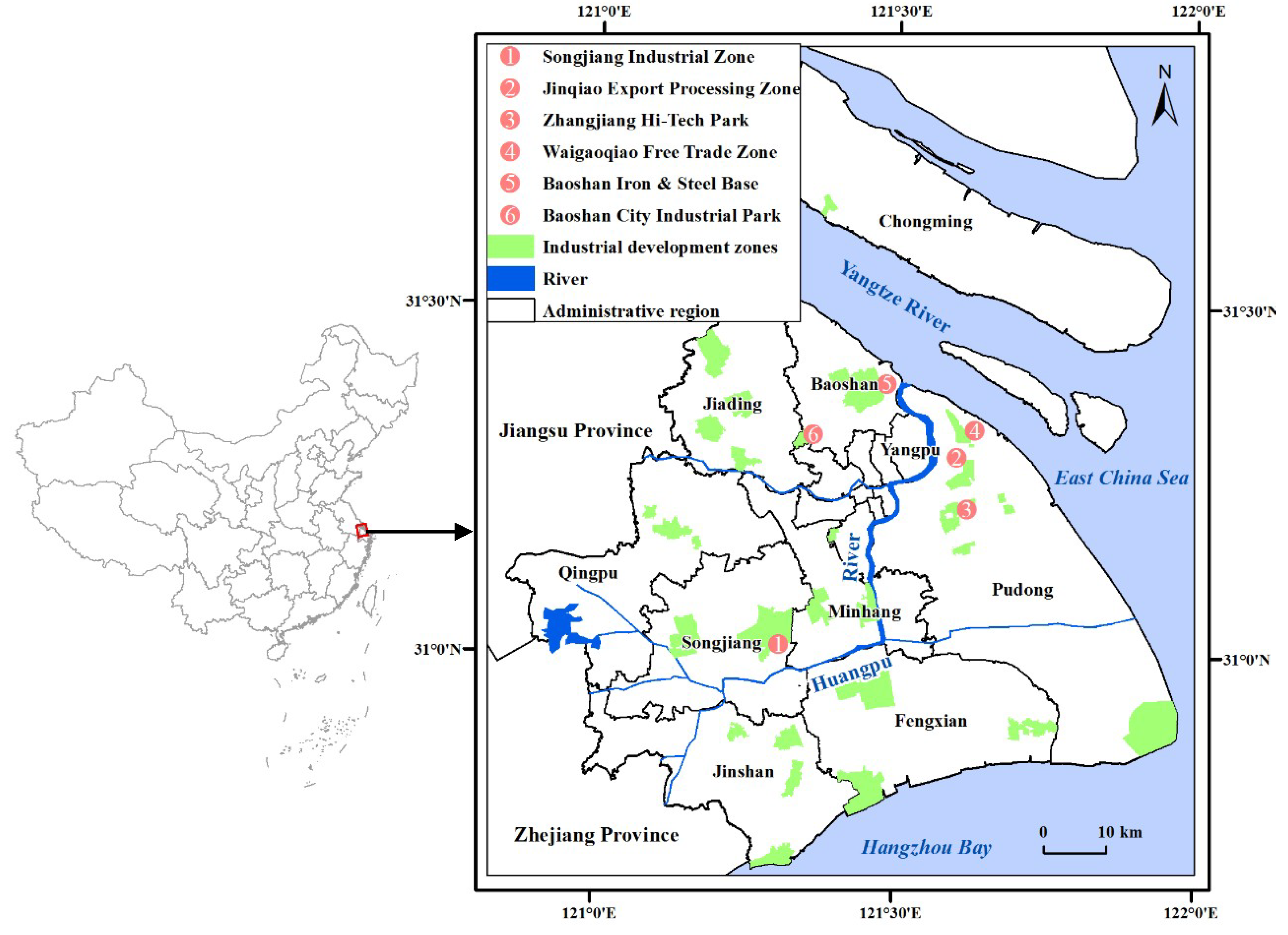
The Shanghai metropolitan area, with a total area of 6340.5 km², is located in the eastern edge of the Yangtze River Delta and is close to the midpoint of the east coastline of China (Figure 1). It is surrounded by water on three sides, with the estuary of the Yangtze River to the north, the East China Sea to the east, and the Hangzhou Bay to the south. The Huangpu River flows through the metropolitan area from west to east in the up-stream and from south to north in the middle- and down-stream. It borders Jiangsu province in northwest and Zhejiang province in southwest, respectively.

Shanghai lies in a flat and low-lying region with an average elevation of 4.0 m, and is frequently threatened by storm surge, storm floods, torrential rainfall and wind brought by typhoon. Since 1949, it has been hit by typhoons around 1.5 times per year and the induced annual flood frequency has increased significantly [27]. In 1905, extreme storm floods led to nearly 30 thousand deaths and injuries in Shanghai [28]. In 1962, extreme storm floods caused 1/6 loss of total GDP in Shanghai. Water level at the Huangpu Park station rose up to 4.76 m and half of the downtown city was inundated for nearly 10 days due to 46 failures (breach and overflowing) points along floodwalls of the Huangpu River and its branches [19,20]. In 1997, Typhoon Winnie led to the direct economic loss of US $100 million in Shanghai. The water level in Huangpu Park rose to 5.72 m, which was equivalent to the water level of the 200 years return period [29]. In 2005, Typhoon Matsa resulted in the accumulative rainfall intensity of 138~350 mm, which caused 238 roads to be under 20~30 cm of inundation and direct economic damage of over US $216 million [20]. In the future, global and local changes are expected to further accelerate the coastal flood risk in Shanghai [11].

Shanghai is one of the most important economic and industrial centers in China. In the past 40 years, the GDP of Shanghai has increased by 108 times. By the end of 2017, its GDP has increased to US $434 billion, accounting for 3.6% of China’s total GDP. GDP density also reaches US $70 million per square kilometer. The manufacturing industry plays an important role in Shanghai, with more than 9000 manufacturing firms above the designated size, 4.1 million employees, an annual added value of US $120 billion, and an annual gross output value of US $490 billion [30]. Many manufacturing firms concentrate in several major industrial development zones that are situated in the riverine and lowland along the Huangpu River (Figure 1). Low-lying terrain as well as dense asset exposure may increase flood risk in these zones.

Table 1. Characteristics of major industrial development zone in Shanghai.

Industrial Zones	Leading Sectors	Area	Fixed Asset	Inventory	Annual Output
		(Sq km)	(billion USD)
Songjiang Industrial Zone	Communication and computers equipment, Fine chemicals;	39.7	4.18	2.43	30.73
Jinqiao Export Processing Zone	Automotive manufacturing, Electronic information, Chemical feedstock and chemical manufacturing;	15.6	3.76	2.59	26.41
Zhangjiang Hi-Tech Park	Bio-medicine, Electronic information;	13.7	3.97	1.98	14.43
Waigaoqiao Free Trade Zone	Electronic information, Automotive parts manufacturing;	9.1	0.23	0.34	2.38
Baoshan Iron & Steel Base	Ferrous metal smelting and extrusion;	39.5	9.45	3.90	14.94
Baoshan City Industrial Park	Automobile parts manufacturing, Metalwork industry	5.6	0.44	0.39	1.49

lists the leading sectors, fixed asset, inventory, and annual output of firms in the major industrial development zones in 2013.

2.2. Data

This study takes manufacturing firms in Shanghai metropolitan area as subjects, covering the section C of the manufacturing industry and subordinate two-digit divisions of C13~C43 (

Table 2. Classification of manufacturing firms with two-digit code.

IND Classes	Two-Digit Manufacturing Divisions	Sector Codes in I-O Table
IND1 Heavy	C30 Non-metallic minerals product industry	S13
	C33 Metalwork industry	S15
	C34 General-purpose equipment manufacturing industry	S16
	C35 Specialized facility manufacturing industry	S17
	C36 Automotive Manufacturing; C37 Railway, marine, aerospace and other transportation equipment manufacturing	S18
	C42 Processing of discarded resources, and waste and scrap recovery	S23
	C43 Metal products, machinery and equipment repair industry	S24
IND2 Light	C17 Textile industry	S07
	C18 Manufacturing industry of textile costumes, shoes, and caps; C19 Manufacturing industry of leather, fur, feather (cloth with soft nap) and their products	S08
	C20 Wood processing and manufacturing industry of wood, bamboo, rattan, palm, and straw-made articles; C21 Cabinetmaking industry	S09
	C22 Papermaking and paper product industry; C23 Printing industry and reproduction of record media; C24 Manufacturing industry for culture, education and sports goods	S10
	C38 Electric machinery and equipment manufacturing industry	S19
	C41 Other manufacturing industries	S22
IND3 Food/Drugs/Chemicals	C13 Manufacturing of agricultural and non-staple foodstuff; C14 Foodstuff manufacturing industry; C15 Beverage manufacturing industry; C16 Tobacco industry	S06
	C25 Petroleum processing, coking and nuclear fuel manufacture	S11
	C26 Chemical feedstock and chemical manufacturing industry; C27 Medicine manufacturing industry; C28 Chemical fiber manufacturing industry; C29 Rubber and plastic production industry	S12
IND4 Metals/Minerals/Processing	C31 Ferrous metal smelting and extrusion; C32 Non-ferrous smelting and extrusion	S14
IND5 High Technology	C39 Manufacturing industry of communication equipment, computers and other electronic equipment	S20
	C40 Manufacturing industry of instruments and meters	S21

) in Chinese Standard Industrial Classification (GB/T 4754-2011). The data is collected from China Industrial Enterprises Database in 2013 published by National Bureau of Statistics [31], which includes all state-owned firms as well as non-state-owned firms with annual revenue above 20 million CNY in China. The database matches the industrial section of the China Statistical Yearbook and the China Industrial Statistics Yearbook, and provides comprehensive and authoritative firm-level data for the study. 8970 manufacturing firms in Shanghai are extracted from the database, including the data items of firm name, address, two-digit code, total asset, fixed asset, inventory, employees, annual output, profit, etc. Fixed assets mainly consist of buildings, equipment and furniture for production. Inventory mainly consists of raw materials, semi-finished and finished goods. The individual firms with two-digit code are subsequently divided into IND1~IND5 classes according to industrial classification in HAZUS-MH system [32], in which the flood depth-damage curves can be utilized for the physical damage assessment. In addition, based on the Input-Output Table of Shanghai in 2012, the individual firms with two-digit code are aggregated into S06~S24 sectors for the ripple loss assessment using IO model.

2.3. Integrated Assessment Framework

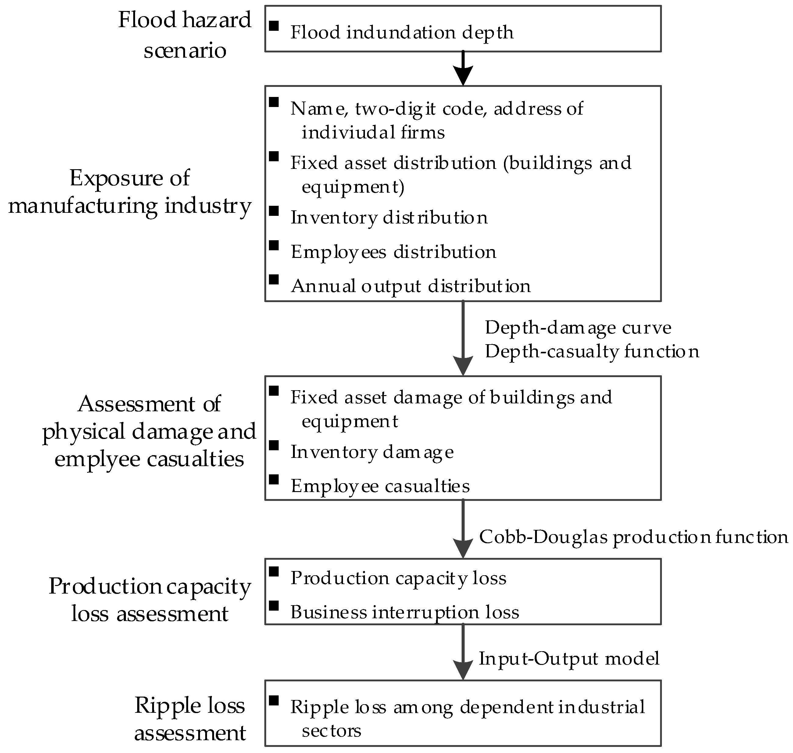
From the perspective of disaster impact propagation in industrial system, this study aims to establish a bottom-up integrated modeling framework to sequentially evaluate the physical damage to industrial facilities of individual firms, the production capacity loss (or business interruption loss) to affected firms/sectors, and the indirect ripple loss in dependent sectors and the entire system (Figure 2). Based on this framework, we can reveal the transfer and amplification effects of economic loss from the local individual firms to the entire industrial system, and identify the most vulnerable/critical nodes for disaster risk prevention.

2.4. Methods

2.4.1. Flood Hazard Scenario

Currently, the DINAS-COAST Extreme Sea Levels (DCESL) dataset [33] and the Global Tide and Surge Reanalysis (GTSR) dataset [34] roughly estimated the extreme sea levels and inundation scenarios of several return periods at a global scale, which covers the coastal areas of Shanghai. In contrast, some other studies simulated the inundation scenarios of storm floods in Shanghai at a precise scale [20,29]. In Ke’s study [20], annual maximum water levels under different return periods (50 year, 100 year, 200 year, 500 year, 1000 year and 10,000 year) at the Wusongkou, Huangpu Park and Mishidu hydrological stations were first calculated using the generalized extreme value (GEV) distribution in hydrological frequency analysis. Then, with the datasets of 30 m resolution DEM and river networks and the boundary conditions of extreme water level, the potential inundation depth and extent along the Huangpu River were simulated using 1D/2D hydrodynamic models embedded in the SOBEK software, including 26 scenarios of no floodwall protection, overtopping, breaching, and failure of floodgates along the river. Considering the spatial scale and the accuracy of the results, we adopt an inundation scenario of a 1000-year flood without floodwall protection simulated by Ke [20]. China’s State Council requires that the main stream of the Huangpu River through the downtown of Shanghai should satisfy the protection standard of a 1000-year flood. However, until now, some parts of the floodwall along the river still have not reached the specific protection standard [35]. Hence, it is of practical significance to discuss the potential impacts of the adopted flood scenario.

The inundation map of a 1000-year flood is directly derived from the simulated results of Ke [20] rather than by running the hydrodynamic models (Figure 3). The map excludes Chongming district (consisting of Chongming island, Changxing island and Hengsha island) due to the lack of boundary conditions of the water level at different return periods. Figure 3 shows that the potential inundation area generally covers the Songjiang and Qingpu districts along the upper reaches of the Huangpu River and Pudong, as well as the Baoshan and Yangpu districts along the lower reaches, with an inundation depth of 0–3.0 m and an area of 606.4 km².

2.4.2. Exposure Analysis of the Manufacturing Industry

Exposure analysis identifies elements that are potentially affected by a certain flood scenario [26]. Flood exposure maps can be multi-scale [14]. For example, administrative units and aggregated statistical datasets are mostly used at country levels. In contrast, land-use or element-based datasets are often desirable at city levels. In this study, firm-level dataset is applied for exposure mapping, which can avoid the possible uncertainty caused by spatial data aggregation. Individual firms are first geocoded with Google API based on their address information and saved as points in an ArcGIS geodatabase (Figure 3). Spatial distribution of fixed asset, inventory and employees are then mapped using ArcGIS.

2.4.3. Assessment of Physical Damage and Employee Casualties

Extreme floods may cause physical damage to industrial facilities such as buildings, equipment, and inventories. One of the main methods for assessing physical damage is the depth-damage curve that describes the relationship between hazard parameters and resulting relative/absolute damage of elements of a certain type or use. HAZUS-MH [36], FLEMO [37], Multicolored Manual [38] and other disaster risk assessment systems all have developed their own flood depth-damage curves for manufacturing industry. However, these functions differ in hazard intensity parameters, classification of elements, resilience factors, spatial scales of application, and loss expression. Unlike FLEMO and Multicolored Manual which take manufacturing industry as a whole, HAZUS-MH classifies industrial facilities into IND1 (Heavy), IND2 (Light), IND3 (Food/Drugs/Chemicals), IND4 (Metals/Minerals Processing), IND5 (High Technology) and IND6 (Construction). This detailed industry classification gives more consideration to the differences of asset exposure and vulnerability in various sectors. In addition, damage in HAZUS-MH system is distinguished as Structure (i.e., building damage), Contents (i.e., equipment damage) and Inventory. Because the post-flood damage data is scarce in the study area, we extract damage data from the latest HAZUS-MH4.0 and fit the depth-damage curves of fixed asset (including buildings and equipment) and inventory. The depth-damage curves are then preliminary calibrated using previous research conducted in Shanghai [19,20]. Next, the damage ratios of fixed asset and inventory for each affected firm are derived from depth-damage curves given inundation depth and manufacturing class. Finally, since the single story buildings are popular in manufacturing sectors, the fixed asset and inventory damage of each firm can be calculated by multiplying its exposed monetary value with damage ratio, respectively. According to the GB/T 4754-2011 of China, the construction industry belongs to section E rather than to section C (the manufacturing industry). Therefore, the damage curve of IND6 is not included in this study.

Extreme floods would also cause employee casualties and labor shortages. Jonkman, et al. [23] developed an empirical exponential function between casualty probability and inundation depth utilizing post-flood survey data in the Netherlands, the UK, the USA and Japan, which can be used to assess the potential employee casualties (Equation (1)).

$$F\left(h\right)=e^{\frac{h-5.58}{0.82}} 0\le h\le 5.58$$

(1)

where h is inundation depth (unit: m), e is the natural constant, $F\left(h\right)$ is casualty probability.

2.4.4. Production Capacity Loss Assessment

Asset damage and labor shortage would further lead to stagnation of production activities and drop of production capacity. Owing to the marginal productivity of input asset and labor, physical damage does not necessarily equal to resulting output loss. Kajitani and Tatano [39], and Yang, et al. [40] developed the empirical production capacity loss ratio (PCLR) models or functional fragility curves for several industrial sectors using firm-level survey data after a certain disaster event. However, these models need to be further verified with large sample size. Koks, et al. [14] established the relationships between output (i.e., value added), capital (i.e., depreciation of fixed asset) and labor (i.e., payment of employees) of different industrial sectors from I-O table by assuming a Cobb-Douglas function with constant returns-to-scale. In this study, in view of the returns-to-scale of individual firms, Cobb-Douglas production functions [41] of IND1~IND5 classes are first developed using a firm-level dataset to simulate the production process that transforms asset and labor factors into the final products (Equation (2)).

$$Q=C{K}^{\alpha }{L}^{\beta }$$

(2)

where Q is the annual output value of individual firms (unit: ten thousand CNY), K is the asset value of individual firms including fixed asset value and inventory value (unit: ten thousand CNY), L is the number of employees of individual firms (unit: person), C is the comprehensive technical coefficient, and α and β are the output elastic coefficients.

Then, using the following Cobb-Douglas function (Equation (3)), we transform the direct damage of asset and labor to output loss for each firm according to IND1~IND5 classes.

$$\mathrm{∆}Q=C\mathrm{∆}{K}^{\alpha }\mathrm{∆}{L}^{\beta }$$

(3)

where ∆Q is the annual output loss of individual firms (unit: ten thousand CNY), ∆K and ∆L are damages of asset (unit: ten thousand CNY) and labor (unit: person), and ∆K consists of fixed asset and inventory damages. For individual firms, annual output loss is the inoperable part of normal annual output, i.e., production capacity loss. Given it needs $T$ years to recover to normal output level, the business interruption loss can be simply expressed as $\mathrm{∆}Q\times T$.

Finally, the annual output losses of affected individual firms are aggregated according to IND1~IND5 manufacturing classes and S06~S24 sectors, respectively.

2.4.5. Ripple Loss Assessment

The drop of production capacity in the manufacturing industry would indirectly trigger ripple loss among dependent industries. The main methods to estimate ripple loss include the IO model [42], CGE model [43,44], Social accounting matrix model (SAM) [45] and Adaptive regional input-output model (ARIO) [22,46]. The IO model is widely used for its simplicity. The CGE model overcomes the limitations of the IO model such as linearity assumption, rigid structure with respect to input and import substitutions, lack of explicit resource constraints, and lack of responses to price changes [13,47]. The SAM model is similar to the IO model, while is rarely applied for the availability of SAM tables [48]. ARIO is a hybrid IO model with CGE characteristics, which allows for production bottlenecks and rationing. In this study, considering the availability of input parameters and the simplicity of its implementation, the IO model is performed to calculate the system-wide ripple loss with the above estimated annual output losses of S06~S24 as input (

Table 3. General structure of I-O table.

Input Sectors	Output Sectors					Final Demand	Total Output
	Sector 1	…	Sector j	…	Sector n
Sector 1	X11		X1j		X1n	Y1	Q1
…
Sector i	Xi1		Xij		Xin	Yi	Qi
Sector j	Xj1		Xjj		Xjn	Yj	Qj
…
Sector n	Xn1		Xnj		Xnn	Yn	Qn
Value added	Z1		Zj		Zn
Total outlays	Q1		Qj		Qn

).

According to Table 3, direct consumption coefficient (i.e., input coefficient) $a_{ij}$ is defined as the input required from the ith sector to produce one unit of production in the jth sector, and is expressed as Equation (4). $a_{ij}s$ constitute matrix A.

$$a_{ij}=X_{ij}/Q_j \left(i,j=1,2,\dots ,n\right)$$

(4)

The full demand coefficient (i.e., inverse matrix coefficient) $b_{ij}$ indicates how much production will be directly and indirectly induced in the ith sector by increasing one unit of final demand in the jth sector. $b_{ij}s$ forms matrix B. The relationship between B and A is shown in Equation (5).

$$B={\left(I-A\right)}^{-1}$$

(5)

where I is an identity matrix.

Given the output loss in the jth sector is $\mathrm{∆}{Q}_j$, the decrease of final demand in the jth sector ($\mathrm{∆}{Y}_j$) is expressed in Equation (6).

$$\mathrm{∆}{Y}_j=\mathrm{∆}{Q}_j/b_{jj}$$

(6)

The output reduction in the ith sector ($\mathrm{∆}{Q}_{ij}$) triggered by the decrease of final demand in the jth sector ($\mathrm{∆}{Y}_j$) is expressed as Equation (7).

$$\mathrm{∆}{Q}_{ij}=b_{ij}\times \mathrm{∆}{Y}_j$$

(7)

Extreme floods may directly affect j (j = 1, 2, … n) manufacturing sectors and indirectly trigger ripple loss to other i (I = 1, 2, … m) industrial sectors. From the column orientation of I-O table, the indirect ripple loss triggered by the jth manufacturing sector ($\mathrm{∆}{Q}_{0j})$ is calculated with Equation (8).

$$\mathrm{∆}{Q}_{0j}={\displaystyle \sum }_{i=1}^m\mathrm{∆}{Q}_{ij}$$

(8)

From the row orientation of I-O table, the indirect ripple loss to the ith sector ($\mathrm{∆}{Q}_{i0})$ is expressed as Equation (9).

$$\mathrm{∆}{Q}_{i0}={\displaystyle \sum }_{j=1}^n\mathrm{∆}{Q}_{ij}$$

(9)

The indirect ripple loss to the entire industrial system ($\mathrm{∆}{Q}_0$) is obtained from Equation (10).

$$\mathrm{∆}{Q}_0={\displaystyle \sum }_{j=1}^n\mathrm{∆}{Q}_{0j}={\displaystyle \sum }_{i=1}^m\mathrm{∆}{Q}_{i0}$$

(10)

3. Results

3.1. Exposure of the Manufacturing Industry

It is calculated that the total asset value of the 8970 firms in Shanghai is about US $424 billion (including fixed asset of US $88 billion and inventory of US $61 billion), the total number of employees is around 4.2 million, and the annual gross output is approximate US $435 billion. The spatial distribution of fixed asset, inventory, and employees are thematically mapped at the aggregated town level (Figure 4).

Figure 4 shows that assets and employees are mostly concentrated in the suburban districts of Pudong, Songjiang, Minhang, Baoshan, Jiading, Fengxian, Qingpu, and Jinshan. The coefficients of variation (CV) of fixed asset, inventory, employee at town level are calculated as 2.35, 1.94 and 1.58, respectively. This means that fixed assets are the most spatially clustered, while employees tend to be relative evenly distributed. Furthermore, annual gross output, fixed asset, inventory and number of employees in the towns where major industrial development zones lie are computed to be about 78.7%, 67.4%, 62.8% and 48.9% of the total manufacturing industry, respectively. These percentages imply that industrial zones play a key role in the regional manufacturing industry, and fixed assets and inventories are more highly concentrated in these major industrial zones than employees.

Sectoral distribution of fixed asset, inventory and employees are then calculated for the top 10 sectors in terms of annual gross output.

Table 4. Sectoral distribution of gross annual output, asset and employees (unit: %).

Two-Digit Divisions	Percentage of Annual Gross Output	Percentage of Fixed Asset	Percentage of Inventory	Percentage of Employee
C39	18.03	12.44	11.05	11.79
C36	16.01	11.54	7.24	7.32
C26	8.67	13.10	6.91	6.26
C34	8.28	9.17	14.82	11.28
C38	7.22	5.61	7.72	9.68
C25	5.84	3.97	3.78	0.69
C31	5.20	11.71	6.39	1.35
C35	3.57	3.73	7.12	5.81
C33	3.17	3.38	3.58	7.17
C29	2.97	3.74	2.97	6.80
Sum	78.96	78.39	71.59	68.13

shows that theses 10 sectors account for a large share of annual gross output, fixed asset, inventory and employees in the entire manufacturing industry. However, individual sectors exhibit different compositions of these shares. For example, C39 has high percentages for all the three input factors while C25 has low shares for all the three. C36, C26 and C31 are characterized with a high percentage of fixed assets, and medium percentages of inventory and employees.

3.2. Physical Damage and Employee Casualties

Based on the data extracted from HAZUS-MH, the depth-damage curves of fixed asset (including buildings and equipment) and inventory for IND1~IND5 are first developed and calibrated, respectively (Figure 5). From Figure 5a, the damage curves of fixed assets for all manufacturing classes present a trend of sharp rises in the inundation depth of 0~1.5m and then a gentle deceleration with further increases of inundation depth. When inundation depth rises to 1.5m, the damage ratio of fixed asset would reach 0.66 for IND3 and IND5, 0.5 for IND2, 0.47 for IND1, and 0.4 for IND4. This means that IND3 and IND5 are more vulnerable to floods than other classes in terms of fixed assets. Figure 5b shows similar trends to Figure 5a except for its much higher damage ratios in the inundation depth of 0~1.5m. At the inundation depth of 1.5 m, the damage ratio of inventory would reach 0.8 for IND3 and IND5, 0.62 for IND2, 0.55 for IND1, and 0.5 for IND4, respectively. It indicates that inventory is more likely to get damaged than fixed assets in this depth range.

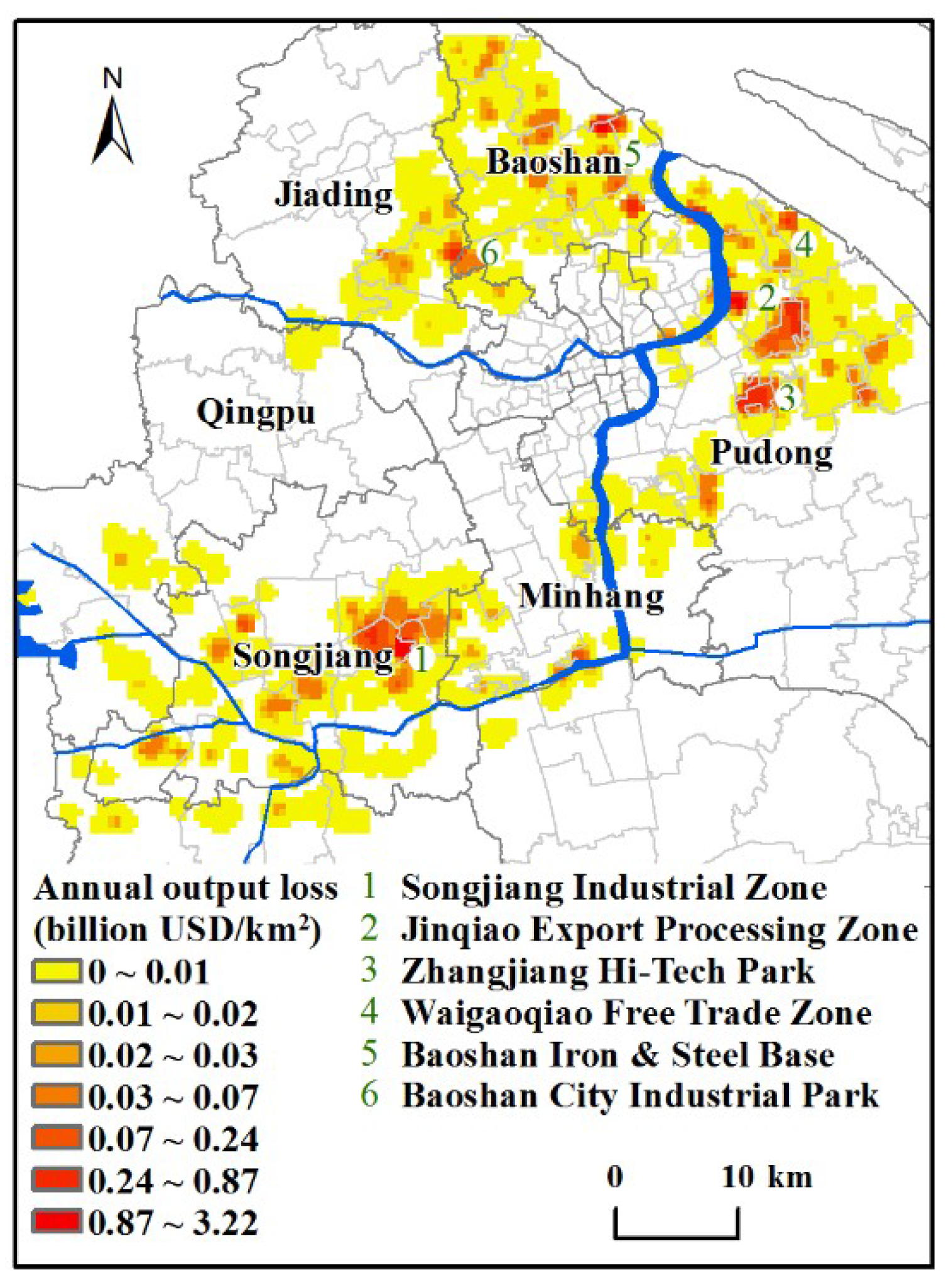
By combining the flood inundation map, the exposure maps of asset and employees, the depth-damage curves of fixed asset and inventory and the depth-casualty function, the potential direct asset damage and employee casualties of individual firms are estimated and mapped using kernel density function in ArcGIS (Figure 6). Figure 6a,b show that extreme floods cause serious damage to manufacturing firms in the Songjiang, Pudong and Baoshan districts, as well as some minor damage in the Jiading, Minhang and Qingpu districts. Several damage hotspots are found in and around key industrial development zones such as Songjiang Industrial Zone, Jinqiao Export Processing Zone, Zhangjiang Hi-Tech Park, Waigaoqiao Free Trade Zone, Baoshan Iron & Steel Base, and Baoshan City Industrial Park. High levels of inundation depth, high density of asset exposure, and water-susceptible industrial structures would jointly contribute to the potential serious damage in these industrial zones. For example, in Songjiang Industrial Zone, fixed asset and inventory per unit are calculated to be US $0.11 billion/km² and US $0.06 billion/km², and the simulated average inundation depth is up to 1.26m. In addition, hardware manufacturing firms of computers, smart phones and communication equipment are extensively located in the zone, which are very susceptible to floods according to Figure 5. Figure 6c indicates that potential employee casualties also concentrate in the industrial development zones mentioned above. However, the spatial pattern of employee casualties presents a lower level of divergence than that of asset damage, which is mainly related to the relative balanced-distribution of employees among sectors and regions.

Finally, the direct damage of affected individual firms is aggregated based on IND1~IND5 classes (

Table 5. Estimation of asset damages and employee casualties of IND1~IND5 classes.

IND Classes	Affected Firms	Fixed Asset Damage (billion USD)	Inventory Damage (billion USD)	Employee Casualties
		∆K		∆L
IND1	724	2.84	1.80	2676
IND2	515	0.77	0.75	1808
IND3	314	1.85	2.40	1003
IND4	420	4.68	2.39	1437
IND5	193	1.85	1.54	1589
Total	2166	11.99	8.88	8513

). As a whole, extreme floods would directly affect 2166 manufacturing firms and cause about fixed asset damage of US $12 billion, inventory damage of US $9 billion, and 8,513 employee casualties, accounting for 24.2%, 13.6%, 14.8% and 0.2% of the total, respectively. The fixed asset damage and inventory damage can be collectively called asset damage (∆K in Table 5).

3.3. Production Capacity Loss

With Equation (2), the Cobb-Douglas functions between annual output (Q), asset (K), and employees (L) of IND1~IND5 manufacturing classes are constructed after eliminating the abnormal firm samples. Afterwards, the asset damage (∆K) and employee casualties (∆L) are taken as input to the Cobb-Douglas functions to calculate the annual output loss (∆Q) for each affected individual firm. The estimated annual output losses (i.e., production capacity loss) of individual firms are then mapped using kernel density function in ArcGIS (Figure 7) and aggregated into IND1~IND5 classes (

Table 6. Coefficients and R² of Cobb-Douglas functions and estimated production capacity loss of IND1~IND5 classes.

IND Classes	C	α	β	R2	∆Q (billion USD)	∆Q/∆K
IND1	0.619	0.921	0.184	0.808	3.73	0.80
IND2	0.621	0.882	0.298	0.716	1.63	1.07
IND3	0.636	0.947	0.229	0.723	5.94	1.40
IND4	0.488	0.896	0.276	0.816	5.11	0.72
IND5	0.645	1.037	0.079	0.897	6.65	1.96

). Table 6 lists the coefficients (C, α, and β) and R² of developed Cobb-Douglas functions, as well as the estimated production capacity loss (∆Q) of IND1~IND5 classes.

From Table 6, the production capacity loss of affected manufacturing firms adds up to about US $23 billion, accounting for 5.3% of the annual industrial gross output of US $435 billion in Shanghai. If excluding labor input, the ratio of ∆Q and ∆K of IND1~IND5 classes is further calculated to reveal the amplification effect from physical damage of input factors to production capacity loss (see Table 6). The ∆Q/∆K ratio is less than 1 for IND1 and IND4, meaning these two manufacturing classes do not have the amplification effect. The ratio is greater than 1 for IND3 and IND5, indicating the amplification effect of the two manufacturing classes is significant. The main reason is that different manufacturing classes have different asset productivity ratios (the ratio of annual output to total asset). The average asset productivity ratios of IND1~IND5 classes in Shanghai are calculated to be 0.83, 1.11, 1.19, 0.87 and 1.45, respectively.

Figure 7 shows that the hot spots of severe production capacity loss still lie in the key industrial development zones mentioned above. However, the ∆Q/∆K ratios are quite different from each other due to each zone’s specific industrial structure. The ratios of Songjiang Industrial Zone, Zhangjiang Hi-Tech Park, Jinqiao Export Processing Zone, Baoshan Urban Industrial Park, and Baoshan Iron & Steel Base are calculated as 2.24, 1.92, 1.25, 0.95 and 0.89, respectively. Taking Songjiang Industrial Zone as an example, asset value and annual output value of C39 account for 63.79% and 77.05% of the total. Its industrial structure dominated by IND5 would lead to a significant amplification effect from asset damage to annual output loss.

3.4. Ripple Loss Among Dependent Industrial Sectors

The aggregated annual output losses of S06~S24 are also derived from the estimated annual output losses of individual firms and used as input (∆Q) to IO model.

Using equation (8), the indirect ripple loss triggered by each damaged manufacturing sector is estimated (

Table 7. Estimation of ripple loss triggered by damaged manufacturing sectors. (unit: billion USD).

Sector Codes	∆Q	∆Y	boj	Ripple Loss	Sector Codes	∆Q	∆Y	boj	Ripple Loss
S06	0.99	0.74	2.50	1.85	S16	0.88	0.75	3.86	2.90
S07	0.07	0.06	3.77	0.23	S17	0.68	0.65	3.70	2.41
S08	0.24	0.21	3.36	0.71	S18	1.86	1.31	3.92	5.14
S09	0.13	0.12	3.60	0.43	S19	0.97	0.84	4.00	3.36
S10	0.27	0.25	3.72	0.93	S20	6.26	3.63	5.09	18.48
S11	1.87	1.40	3.11	4.35	S21	0.38	0.36	3.49	1.26
S12	3.46	1.98	3.68	7.29	S22	0.02	0.01	3.31	0.03
S13	0.37	0.33	2.97	0.98	S23	0.06	0.03	4.03	0.12
S14	3.93	2.19	3.45	7.56	S24	0.03	0.02	3.36	0.07
S15	0.59	0.49	3.54	1.73	Total	23.06	15.37		59.80

). In Table 7, b_0j is the column total of inverse matrix coefficients related to the jth manufacturing sector, representing the output increment of the entire industrial system with one unit of final demand in the jth manufacturing sector. b_0j varies from 2.50 to 5.09 in the study area, indicating that manufacturing sectors have strong linkage effects in regional industrial system. The manufacturing sectors with high b_0j such as S20 (Communication equipment, computers and other electronic equipment), S19 (Electric machinery and equipment manufacturing industry), S18 (Transportation equipment industry), S16 (General-purpose equipment manufacturing industry) and S17 (Specialized facility manufacturing industry) are not only the leading and driving forces of regional economic growth, but also the most vulnerable and critical nodes for disaster risk prevention. Much more attention should be paid to the system-wide ripple loss triggered by direct damage of these critical manufacturing sectors. Table 7 also implies that the ripple losses triggered by S20, S14 (Metal smelting and calendaring products), S12 (Chemical products), S11 (Petroleum, coking and nuclear fuel processing products), S18, S19, S16, S17, and S06 (Food and tobacco) are the largest owing to their greater annual output losses (∆Q) and higher b_0j values.

The ripple loss to each related industry is also estimated with equation (9) (

Table 8. Estimation of ripple loss among dependent industries (unit: billion USD).

Indirect Affected Industries	bi0	Ripple Loss	Indirect Affected Industries	bi0	Ripple Loss
A Farming, forestry, animal husbandry and fishery	0.27	0.16	K Realty business	0.48	0.37
B Mining industry	5.38	5.55	L Leasehold and business service industry	2.55	1.90
C Manufacturing industry	49.42	43.76	M Scientific research, technical service and geologic examination industry	0.09	0.07
D Production and supply of electric power, gas and water	2.62	1.97	N Water conservancy, environment and public institution management	0.01	0.01
E Construction industry	0.07	0.05	O Neighborhood services and other service industry	0.28	0.21
F Wholesale and retail trade	1.89	1.67	P Education	0.04	0.03
G Traffic, storage and mail business	2.36	1.74	Q Sanitation, social security and social welfare industry	0.01	0.01
H Accommodation and food industry	0.35	0.25	R Cultural, physical and entertainment industry	0.03	0.02
I Information transfer, computer service and software industry	0.83	0.59	S Public administration and social organization	0.03	0.03
J Finance industry	1.76	1.41	Total		59.80

). In Table 8, b_i0 is the row total of inverse matrix coefficients associated with the ith industry and stands for its output increment when all related manufacturing sectors simultaneously increase one unit of final demand. From Table 8, b_i0 of the manufacturing industry (C) is up to 49.42 because sectors within the manufacturing industry are highly dependent, and are then followed sequentially by the industries of B, D, L, and G.

Using Equation (10), the system-wide ripple loss is estimated to be about US $60 billion which is 2.6 times of the annual output loss of manufacturing industry. It clearly shows a significant multiplier effect from the production capacity loss to ripple loss. Hence, attention should be paid not only to the direct damage and production capacity loss within manufacturing industry but also to the ripple impacts on related industries.

4. Discussions

How to reasonably simulate direct loss and indirect loss as a function of increasing hazard intensity is highly concerned by the academic community. In this study, an integrated framework is proposed for assessing physical damage, production capacity loss and inter-sector ripple loss coupling depth-damage curve, Cobb-Douglas production function and IO model.

The integrated methodology in this paper presents the following improvements over previous studies. First, detailed firm-level census data rather than land use or administrative region data are applied to exposure analysis and mapping, which eliminates the assumption of evenly distribution of asset value within a certain land use type. It also avoids the disaggregation of economic statistics and the likely consequent uncertainty. Second, instead of taking the manufacturing industry as a whole, classified depth-damage curves are developed to assess the physical damage of fixed assets and inventory for different manufacturing classes. This reveals the differences of asset exposure and vulnerability of various sectors within the manufacturing industry. Third, production capacity loss (i.e., flow loss) rather than physical damage (i.e., stock loss) is used as an input to the IO model, which takes the marginal productivity of input factors into consideration. Classified Cobb-Douglas production functions are applied to transform the physical damages of asset and labor into production capacity loss. Cobb-Douglas functions are built based on individual firm data from which differences in returns-to-scale at firm level are concerned. This approach overcomes the weakness of constant returns-to-scale assumption [14] Finally, IO model is utilized in this study not only to evaluate the system-wide indirect ripple loss triggered by affected manufacturing industry, but also to identify the most vulnerable and critical sectors (nodes) within the regional industrial networks for disaster risk prevention.

However, there are still some uncertainties and problems to be studied in the future. First, the damage curve is recognized as the primary source of uncertainty in flood damage estimation [49]. Because of the lack of detailed and reliable post-flood loss data in the study area, the depth-damage curves used for physical damage assessment are mainly developed from HAZUS-MH, which need to be further localized and calibrated in the future. Second, Cobb-Douglas function is performed to transform physical damage into annual output loss. Different understandings and parameter settings in the Cobb-Douglas function may lead to uncertainty in annual output loss estimation. It is essential to develop optimal production functions for different sectors and regions based on their specific characteristics. Third, IO model and CGE model are commonly used for the indirect system-wide ripple loss assessment. The estimated ripple loss obtained from IO model can be further compared and verified with the CGE model.

5. Conclusions

From the perspective of ex-ante risk analysis, we develop an integrated multi-process and multi-scale assessment methodology for economic loss evaluation caused by floods in the manufacturing industry. Given a hazard intensity scenario, the resulting physical damage, production capacity loss and inter-sector ripple loss can be estimated successively.

The results show that, given no floodwall protection, a scenario of a 1000-year storm flood would cause approximate direct asset damages of US $21 billion to affected manufacturing firms, including fixed asset damage of US $12 billion and inventory damage of US $9 billion. The damage hotspots are found in and around several key industrial development zones, due to their high level of inundation depth, high density of asset exposure, and water-susceptible industrial structure. The shortage of input productive factors of asset and labor would further lead to production capacity loss of US $25 billion to affected manufacturing firms/sectors. During the transformation from physical damage to production capacity loss, the amplification ratio varies across manufacturing classes and industrial development zones with specific structures. In addition, the affected manufacturing industry would indirectly result in ripple losses of US $60 billion among dependent sectors, which implies a significant multiplier effect. Our results have important implications for reasonable cost-benefit analysis of structural flood control measures such as dike upgrading and tidal barrier construction of Huangpu River, as well as for manufacturing firm location planning and resilience strategy decision-making.

References

1. Haraguchi, M.; Lall, U. Flood risks and impacts: A case study of Thailand’s floods in 2011 and research questions for supply chain decision making. Int. J. Disaster Risk Reduct. 2014, 14, 256–272. [Google Scholar] [CrossRef]
2. Hall, T.M.; Sobel, A.H. On the impact angle of Hurricane Sandy’s New Jersey landfall. Geophys. Res. Lett. 2013, 40, 2312–2315. [Google Scholar] [CrossRef]
3. Schröter, K.; Kunz, M.; Elmer, F.; Mühr, B.; Merz, B. What made the June 2013 flood in Germany an exceptional event? A hydro-meteorological evaluation. Hydrol. Earth Syst. Sci. 2015, 19, 309–327. [Google Scholar] [CrossRef] [Green Version]
4. Zhang, W.; Villarini, G.; Vecchi, G.A.; Smith, J.A. Urbanization exacerbated the rainfall and flooding caused by hurricane Harvey in Houston. Nature 2018, 563, 384. [Google Scholar] [CrossRef] [PubMed]
5. Balica, S.F.; Wright, N.G.; van der Meulen, F. A flood vulnerability index for coastal cities and its use in assessing climate change impacts. Nat. Hazards 2012, 64, 73–105. [Google Scholar] [CrossRef] [Green Version]
6. Hallegatte, S.; Green, C.; Nicholls, R.J.; Corfee-Morlot, J. Future flood losses in major coastal cities. Nat. Clim. Chang. 2013, 3, 802–806. [Google Scholar] [CrossRef]
7. Hartmann, D.L.; Tank, A.M.K.; Rusticucci, M.; Alexander, L.V.; Brönnimann, S.; Charabi, Y.A.R.; Dentener, F.J.; Dlugokencky, E.J.; Easterling, D.R.; Kaplan, A. Observations: Atmosphere and surface. In Climate Change 2013: The Physical Science Basis. Working Group I Contribution to the Fifth Assessment Report of the Intergovernmental Panel on Climate Change; Stocker, T.F., Qin, D., Plattner, G.K., Tignor, M., Allen, S.K., Boschung, J., Nauels, A., Xia, Y., Bex, V., Midgley, P.M., Eds.; Cambridge University Press: Cambridge, UK, 2013; pp. 159–254. [Google Scholar]
8. Rahmstorf, S. Rising hazard of storm-surge flooding. Proc. Natl. Acad. Sci. USA 2017, 114, 11806–11808. [Google Scholar] [CrossRef] [PubMed] [Green Version]
9. Wang, J.; Gao, W.; Xu, S.; Yu, L. Evaluation of the combined risk of sea level rise, land subsidence, and storm surges on the coastal areas of Shanghai, China. Clim. Chang. 2012, 115, 537–558. [Google Scholar] [CrossRef]
10. Yin, J.; Yu, D.; Wilby, R. Modelling the impact of land subsidence on urban pluvial flooding: A case study of downtown Shanghai, China. Sci. Total. Environ. 2016, 544, 744–753. [Google Scholar] [CrossRef] [Green Version]
11. Wang, J.; Yi, S.; Li, M.; Wang, L.; Song, C. Effects of sea level rise, land subsidence, bathymetric change and typhoon tracks on storm flooding in the coastal areas of Shanghai. Sci. Total. Environ. 2018, 621, 228–234. [Google Scholar] [CrossRef]
12. Hallegatte, S. The Indirect Cost of Natural Disasters and an Economic Definition of Macroeconomic Resilience. Available online: http://documents.worldbank.org/curated/en/186631467998501319/pdf/WPS7357.pdf (accessed on 7 December 2018).
13. Rose, A. Economic principles, issues, and research priorities in hazard loss estimation. In Modeling Spatial and Economic Impacts of Disasters; Springer: Berlin, Germany, 2004; pp. 13–36. [Google Scholar]
14. Koks, E.E.; Bočkarjova, M.; Moel, H.D.; Aerts, J.C. Integrated direct and indirect flood risk modeling: Development and sensitivity analysis. Risk Anal. 2015, 35, 882–900. [Google Scholar] [CrossRef] [PubMed]
15. Pérez, L.P.; Hurlé, J.B. Assessing the socio-economic impacts of drought in the Ebro River Basin. Span. J. Agric. Res. 2009, 7, 269–280. [Google Scholar] [CrossRef]
16. Meyer, V.; Becker, N.; Markantonis, V.; Schwarze, R.; Van den Bergh, J.; Bouwer, L.; Bubeck, P.; Ciavola, P.; Genovese, E.; Green, C. Review article: Assessing the costs of natural hazards–state of the art and knowledge gaps. Nat. Hazards Earth Syst. Sci. 2013, 13, 1351–1373. [Google Scholar] [CrossRef]
17. Li, W.; Wen, J.; Li, X. Progress of research on economic loss assessment of disasters in industrial networks. Prog. Geogr. 2018, 37, 330–341. (In Chinese) [Google Scholar]
18. Yi, C.S.; Lee, J.H.; Shim, M.P. GIS-based distributed technique for assessing economic loss from flood damage: Pre-feasibility study for the Anyang Stream Basin in Korea. Nat. Hazards 2010, 55, 251–272. [Google Scholar] [CrossRef]
19. Yin, J.; Yin, Z.E.; Yu, D.P.; Yuan, X.S. Vulnerability analysis for storm induced flood: A case study of Huangpu River Basin. Sci. Geogr. Sin. 2012, 32, 1155–1160. (In Chinese) [Google Scholar]
20. Ke, Q. Flood Risk Analysis for Metropolitan Areas: A Case Study for Shanghai; Delft Academic Press: Delft, The Netherlands, 2014. [Google Scholar]
21. Zeleňáková, M.; Gaňová, L.; Purcz, P.; Horský, M.; Satrapa, L. Determination of the potential economic flood damages in Medzev, Slovakia. J. Flood Risk Manag. 2018, 11, S1090–S1099. [Google Scholar] [CrossRef]
22. Wu, J.; Li, N.; Hallegatte, S.; Shi, P.; Hu, A.; Liu, X. Regional indirect economic impact evaluation of the 2008 Wenchuan Earthquake. Environ. Earth Sci. 2012, 65, 161–172. [Google Scholar] [CrossRef]
23. Jonkman, S.; Bočkarjova, M.; Kok, M.; Bernardini, P. Integrated hydrodynamic and economic modelling of flood damage in the Netherlands. Ecol. Econ. 2008, 66, 77–90. [Google Scholar] [CrossRef]
24. Carrera, L.; Standardi, G.; Bosello, F.; Mysiak, J. Assessing direct and indirect economic impacts of a flood event through the integration of spatial and computable general equilibrium modelling. Environ. Model. Softw. 2015, 63, 109–122. [Google Scholar] [CrossRef] [Green Version]
25. Yang, S.Y.; Chan, M.H.; Chang, C.H.; Chang, L.F. The damage assessment of flood risk transfer effect on surrounding areas arising from the land development in Tainan, Taiwan. Water 2018, 10, 473. [Google Scholar] [CrossRef]
26. Merz, B.; Kreibich, H.; Schwarze, R.; Thieken, A. Review article: Assessment of economic flood damage. Nat. Hazards Earth Syst. Sci. 2010, 10, 1697–1724. [Google Scholar] [CrossRef]
27. Du, S.; Gu, H.; Wen, J.; Chen, K.; Van Rompaey, A. Detecting flood variations in Shanghai over 1949–2009 with Mann-Kendall tests and a newspaper-based database. Water 2015, 7, 1808–1824. [Google Scholar] [CrossRef]
28. Yuan, Z. Flood and Drought Disasters in Shanghai; Hohai University Press: Nanjing, China, 1999. (In Chinese) [Google Scholar]
29. Ke, Q.; Jonkman, S.; van Gelder, P.; Bricker, J. Frequency Analysis of Storm-Surge-Induced Flooding for the Huangpu River in Shanghai, China. J. Mar. Sci. Eng. 2018, 6, 70. [Google Scholar] [CrossRef]
30. Shanghai Municipal Statistics Bureau. Shanghai Statistical Yearbook; China Statistics Press: Beijing, China, 2018. (In Chinese)
31. Nie, H.; Jiang, T.; Yang, R. A review and reflection on the use and abuse of Chinese Industrial Enterprises Database. World Econ. 2012, 5, 142–158. (In Chinese) [Google Scholar]
32. FEMA. Multi-Hazard Loss Estimation Methodology: Flood Model Technical Manual. Available online: https://www.fema.gov/media-library-data/20130726-1820-25045-8292/hzmh2_1_fl_tm.pdf (accessed on 7 December 2018).
33. Vafeidis, A.T.; Nicholls, R.J.; McFadden, L.; Tol, R.S.; Hinkel, J.; Spencer, T.; Grashoff, P.S.; Boot, G.; Klein, R.J. A new global coastal database for impact and vulnerability analysis to sea-level rise. J. Coast. Res. 2008, 24, 917–924. [Google Scholar] [CrossRef]
34. Muis, S.; Verlaan, M.; Nicholls, R.J.; Brown, S.; Hinkel, J.; Lincke, D.; Vafeidis, A.T.; Scussolini, P.; Winsemius, H.C.; Ward, P.J. A comparison of two global datasets of extreme sea levels and resulting flood exposure. Earth’s Future 2017, 5, 379–392. [Google Scholar] [CrossRef] [Green Version]
35. Liu, M.; Wang, J.; Yin, J. Study on the urban safety and comprehensive disaster prevention in Shanghai. Shanghai Urban Plan. 2016, 1, 1–8. (In Chinese) [Google Scholar]
36. Scawthorn, C.; Flores, P.; Blais, N.; Seligson, H.; Tate, E.; Chang, S.; Mifflin, E.; Thomas, W.; Murphy, J.; Jones, C. HAZUS-MH flood loss estimation methodology. II. Damage and loss assessment. Nat. Hazards Rev. 2006, 7, 72–81. [Google Scholar] [CrossRef]
37. Kreibich, H.; Seifert, I.; Merz, B.; Thieken, A.H. Development of FLEMOcs—A new model for the estimation of flood losses in the commercial sector. Hydrol. Sci. J. 2010, 55, 1302–1314. [Google Scholar] [CrossRef]
38. Penning-Rowsell, E.; Johnson, C.; Tunstall, S.; Tapsell, S.; Morris, J.; Chatterton, J. The Benefits of Flood and Coastal Risk Management—A Manual of Assessment Techniques; Middlesex University Press: London, UK, 2005. [Google Scholar]
39. Kajitani, Y.; Tatano, H. Estimation of production capacity loss rate after the great East Japan earthquake and tsunami in 2011. Econ. Syst. Res. 2014, 26, 13–38. [Google Scholar] [CrossRef]
40. Yang, L.; Kajitani, Y.; Tatano, H.; Jiang, X. A methodology for estimating business interruption loss caused by flood disasters: Insights from business surveys after Tokai Heavy Rain in Japan. Nat. Hazards 2016, 84, 411–430. [Google Scholar] [CrossRef]
41. Hallegatte, S.; Vogt-Schilb, A. Are Losses from Natural Disasters More than Just Asset Losses? Available online: http://101.96.10.63/documents.worldbank.org/curated/en/488681478879461092/pdf/WPS7885.pdf (accessed on 7 December 2018).
42. Li, J.; Crawford-Brown, D.; Syddall, M.; Guan, D. Modeling imbalanced economic recovery following a natural disaster using Input-Output analysis. Risk Anal. 2013, 33, 1908–1923. [Google Scholar] [CrossRef] [PubMed]
43. Rose, A.; Liao, S.Y. Modeling regional economic resilience to disasters: A computable general equilibrium analysis of water service disruptions. J. Reg. Sci. 2005, 45, 75–112. [Google Scholar] [CrossRef]
44. Kajitani, Y.; Tatano, H. Applicability of a spatial computable general equilibrium model to assess the short-term economic impact of natural disasters. Econ. Syst. Res. 2017, 30, 1–24. [Google Scholar] [CrossRef]
45. Cole, S. Lifelines and livelihood: A social accounting matrix approach to calamity preparedness. J. Conting. Crisis Manag. 1995, 3, 228–246. [Google Scholar] [CrossRef]
46. Hallegatte, S. An adaptive regional Input-Output model and its application to the assessment of the economic cost of Katrina. Risk Anal. 2008, 28, 779–799. [Google Scholar] [CrossRef]
47. Okuyama, Y. Economic modeling for disaster impact analysis: Past, present, and future. Econ. Syst. Res. 2007, 19, 115–124. [Google Scholar] [CrossRef]
48. Koks, E.; Carrera, L.; Jonkeren, O.; Aerts, J.; Husby, T.; Thissen, M.; Standardi, G.; Mysiak, J. Regional disaster impact analysis: Comparing Input-Output and Computable General Equilibrium models. Nat. Hazards Earth Syst. Sci. 2015, 3, 7053–7088. [Google Scholar] [CrossRef]
49. De Moel, H.; Aerts, J. Effect of uncertainty in land use, damage models and inundation depth on flood damage estimates. Nat. Hazards 2011, 58, 407–425. [Google Scholar] [CrossRef]
Figure 1. Map of study area.
Sustainability 11 00126 g001
Figure 2. Integrated assessment framework.
Sustainability 11 00126 g002
Figure 3. Flood inundation scenario (from Ke [20]) and distribution of manufacturing firms.
Sustainability 11 00126 g003
Figure 4. Spatial distribution of asset and employees of Shanghai manufacturing industry.
Sustainability 11 00126 g004
Figure 5. Flood depth-damage curves for IND1~IND5 classes.
Sustainability 11 00126 g005
Figure 6. Spatial distribution of asset damage and employee casualties.
Sustainability 11 00126 g006
Figure 7. Spatial distribution of production capacity loss.
Sustainability 11 00126 g007