Abstract
The carbon market is the least-cost tool to reduce carbon emissions. This study explores the evolution of the carbon price in the carbon market from a dynamic system perspective. A three-dimensional carbon price dynamic system is established to quantify the interactions among the carbon price, energy price, and economic growth. The system built in this study presents various dynamic characteristics including chaotic attractors and stable equilibria. Specifically, the existence of chaos in the system is verified by Lyapunov exponents spectrum and bifurcation diagram. In contrast, the system tends to be stable in the case of China after identifying the system parameters through the genetic algorithm. Furthermore, evolutionary trends of the carbon price are analyzed when the system parameters are perturbed. The results show that the carbon price is positively correlated with energy price as well as energy price policy. Besides, the level of the carbon price is negatively correlated with government control in the short term and positively correlated in the long term. This study can help analyze trends in the carbon price in the mid-term to long-term.
1. Introduction
Reducing carbon dioxide emissions is the key to curbing climate warming. This has been widely acknowledged by the international community after the announcement of “the United Nations framework convention on climate change” [1]. The European Community plus 37 industrialized nations are mandated to cut their greenhouse gas emissions under the Kyoto Protocol [2]. Market mechanisms have become a new pathway to reduce carbon dioxide emissions since the European Union created the world’s first major carbon market in 2005. China announced its initiation of carbon trading pilots in June 2013. In carbon markets, carbon emissions are conceptualized as a tradable commodity. This kind of marketization encourages enterprises to transform to low-carbon energy consumption, actively promote technological innovation, and strictly control carbon emissions, thereby promoting low-carbon development [3].
The market needs a gradually increasing carbon price to provide long-term signals to market participants. The carbon price is essentially affected by factors from the demand side, such as energy prices [4], the macroeconomic environment [5], policy factors [6,7], prices of related products [8], climate change [9], and foreign direct investment [10]. Energy price and economic growth are regarded as the most important influencing factors.
The existing literature shows that energy prices and carbon prices have strong, positive in most cases, correlations. Convery and Redmond [11] found that energy price is the primary factor impacting on carbon price volatility in the EU market of the first phase. The U.S. Regional Greenhouse Gas Initiative market is loosely tied with the electricity market, unlike the EU-ETS [12]. There are bi-directional and time-varying spillovers between carbon and energy markets. For example, Zhang and Sun [13] applied DCC-TGARCH model and full BEKK-GARCH model to investigate the dynamic volatility spillover between carbon and energy prices, and found out that coal market had the highest positive correlation with the carbon market. Kanamura [14] examined the role of carbon swap trading and energy prices in price correlations and volatilities between carbon markets. The study showed stronger energy price impacts on EUA prices than CER prices and a positive energy price impact on EUA prices. Sousa et al. [15] characterized the interrelation of CO prices with energy prices using multivariate wavelet analysis.
A growing economy affects carbon price through stimulating fossil fuel consumption. Economic growth is the dominant determinant of the carbon price in the long term. It is estimated that a persistent 10% drop in annual GDP growth would lead to a 4.0–4.5% fall in EUA prices [16]. The regional shadow prices are positively correlated with the level of economic development in Chinese provinces [17]. Carbon price in Beijing pilot was found to have a positive correlation with economic development by using a structural VAR model [18]. When considering the constraints of the carbon price, economic growth will be hampered in the near future [19]. Fan and Todorova [20] found the positive correlation of allowance prices with utilities, industrial and materials sector indices in some of China’s pilot carbon markets. Guo et al. [21] constructed GARCH models to investigate the comoves between the micro-behaviors and carbon prices. Their microeconomic findings confirm the maturity of EU ETS in the second phase.
Studies on the effect from a combination of factors have attracted an increasing attention in the literature. Tan and Wang [5] expounded the quantile-based dependence dynamics of EUA-energy and EUA-macro economy, and analyzed the influence paths from energy and financial markets to carbon markets in the different phase of EU ETS. Chevallier [22] simulated carbon price dynamics in response to economic activity and energy price, confirming the link between macroeconomic and carbon price and revealing new interactions between carbon price, macroeconomic and energy variables.
Fluctuation in carbon price presents both linear and nonlinear way due to inherently high complexity. Carbon price dynamics is usually described as stochastic processes by econometrical methods and soft-computing models [23,24,25]. To understand the adjustment of carbon prices in the economic environment and energy market, Zhao et al. [2] established a real-time prediction program to study carbon price forecasting. The evidence shows that mixed frequency economy and energy data are useful for predicting carbon price. A chaotic phenomenon was found in European carbon market [26]. In general, we hypothesize that carbon price presents complex behavior characteristics in its evolution.
This study uses the nonlinear dynamical system to explore the evolution of the carbon price in the carbon market. Such a system well reflects the nonlinearity underlying the dynamics of the price. Most of the previous studies on carbon price mainly use methods and models from the perspective of statistics and econometrics. Few studies use quantitative analysis to research the influence on the carbon price, energy price and economic growth. Studies from a dynamic growth perspective provide new sights in the complex interaction between the energy price and economic growth [27]. Using a two-sector endogenous growth model, Berk and Yetkiner showed the negative impact of the growth rate of energy prices on those of energy use and real GDP. Weber et al. [28] investigated the interactions between climate and the socioeconomic system through a Multi-Actor Dynamic Integrated Assessment Model. Nonlinear dynamical system, describing changes in variables over time, may appear chaotic, unpredictable or counterintuitive, contrasting with much simpler linear systems. It is used to describe the behavior of complex dynamic systems, usually using a nonlinear system of equations. Researches on the complexity of economic systems using nonlinear dynamics theory have yielded many results. Fang et al. [29] built a three-dimensional dynamic system under the interrelationship between energy-saving and emission-reduction, carbon emissions and economic growth. They found a series of findings [19,30,31]. Zhang and Tian [32] established a three-dimensional nonlinear dynamic system about energy price, energy efficiency and economic growth. Wang and Tian [33] proposed a three-dimensional dynamic system of energy prices, energy supply, and economic growth. Fan et al. [34] put forward a REP dynamical system through the close relationship between resources, economic growth, and pollution. These studies provide a sound theoretical basis for this paper.
The chaotic behavior is of great importance for the sustainability of a complex system. Chaotic behavior may occur at non-equilibrium states [35] when the system evolves because of the nonlinearity and dynamic nature of sustainable development. Therefore chaos happens in the backdrop of sustainability in the case of complex systems. However, there is no contradiction existing between chaos and sustainability as chaotic systems are stable on the system scale [36]. Thus, chaos and sustainability are synthesized as two poles in the development of a complex system [37], considering that chaos destroys sustainability, and sustainability belies chaos in the local scale. Strange attractors, the key indicator of a chaotic system, could be the most apt description of a sustainably developing system [38]. The unpredictable characteristic of chaos means that the objective is to stay on the sustainable state represented by the attractor [38]. Based on these senses, it is concluded that the phenomenon of chaos represents sustainability [39]. In fact, the theory of “edge of chaos ” [40] shows that the system develops towards sustainability in a perpetual exploration of emergent order moving from chaos into order and back again. Chaos may be resulted by different parameter values of the system, or its initial conditions once the system has been regarded as chaotic. This paper shows a variety of parameter conditions leading to chaotic behavior. Policy implications for sustainability could be made beyond those conditions.
The purpose of this paper is to study the evolutionary trends of the carbon price from a nonlinear dynamical system perspective. For this aim, we construct a three-dimensional nonlinear carbon price dynamic system based on the complex relationships among carbon price, energy price, and economic growth. Then we obtain the conditions for chaos by dissipative analysis and parameter analysis. Lyapunov exponents spectrum and bifurcation diagram verify the existence of chaos. Finally, the evolutionary trends of the carbon price dynamical system are shown under parameter perturbations. The main contribution can be divided into three aspects. Firstly, a three-dimensional carbon price dynamic system is constructed and the nonlinear dynamics theory is applied to analyze the dynamic characteristics of the system. Secondly, an example system is obtained based on China’s statistical data with the aid of the genetic algorithm. The result shows that the example system is stable, in line with the case in China. Thirdly, this paper explores the evolving actions of carbon price system through disturbance parameters, and further studies the dynamic behavior between carbon price and each variable. The proposal to discuss the development path of the carbon price is beneficial to improve the price mechanism of the carbon market, accumulate experience in gradually increasing carbon price, and promote China’s low-carbon development.
The outline of this paper is organized as follows: Section 2 is about the establishment of the carbon price dynamic system. Section 3 discusses the dynamic characteristics of the system. Section 4 provides a case study based on China’s statistic data. The impact of parameters on system variables is shown in Section 5. Conclusions are presented in Section 6.
2. The Carbon Price Dynamic System
We make some assumptions for the modelling. Firstly, we assume that economic output is only generated by the energy industry, mainly for social consumption and energy consumption. Secondly, we only consider fossil fuels such as coal and oil, and low-carbon energy is temporarily neglected. Thirdly, we assume that there are only spot prices of carbon emissions and all the traders are emissions firms in the carbon market.
2.1. Causal Relationships between Carbon Price, Energy Price and Economic Growth
Carbon price system is a complicated system containing many factors, such as carbon price, economic growth, energy price, policy adjust, supply and demand, and energy structure. These factors are interdependent and mutually constrained. Figure 1 presents an illustration of such relationships, where the boxes represent variables and factors, () represents the conductive relationships of factors, a plus sign “+” means positive correlation, and a minus sign “−” means negative correlation. An increase in carbon price leads to a drop in economic development and energy price. It stimulates technology innovation which will effectively narrow the gap between supply and demand of carbon emission and lower energy prices. The decline in energy prices cuts energy production and leads to a slowdown in economic development. On the other hand, the increase in economic growth causes a sequential increase in carbon emissions and carbon price. To control the excessive carbon price, policy regulations are adjusted to improve the energy structure, promote the development of low-carbon activities, and grantee a growing economy. As the economy develops, total productivity and energy price rise which will promote scientific and technological progress. In addition, the increase in energy price can also promote the exploitation of new energy, thereby increasing low-carbon activities. Therefore, there exists direct and indirect complicated nonlinear conductive relationships among carbon price, energy price, and economic growth.
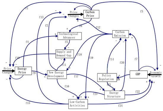
Figure 1.
The causal relationship among the variables of the carbon price system.
2.2. Model Structure
This subsection establishes a nonlinear differential equation system to quantify the evolution of the dominant variables of the carbon price system.
It has been well acknowledged to consider carbon price, energy price and economic output in a time-varying background. Let represent the carbon price, , the energy price, , the economic output in an economy, , T is a given economic period. We set up a differential equation model because that it is the economic growth rather the output is the attention of the economy.
By the first assumption, the derivative of the economic output is a function of the output, the energy price, and the carbon price, that is, Intuitively, F includes a logistic term based on the limited growth theory. The partial derivative represents the economic coefficient of the carbon price. Its value should be negative as we see that has a negative sign in Figure 1, meaning the increase of carbon price can cut back economic growth directly. The partial derivative represents the economic coefficient of energy price. The increase of energy price can promote new energy development (see in Figure 1), where the new energy development can boost economic growth ( see and ) through adjusting energy structure (see ) and low-carbon activities (see and ). Therefore, is some positive function of , and . Combining the above analysis, we have
Next, we consider . Energy price has an increasing trend in the long run, indicating . It is known from Figure 1 that the increase of carbon price can undermine energy prices (see ) and narrow the gap between supply and demand of carbon emission (see ) through technology advances (see ). Thus the influence of carbon price on energy price is negative, that is, . A logistic term is included in G since the economic output is only generated from energy consumption by the first assumption. Then we have
Finally, we consider . A stable while relatively increasing carbon price is beneficial for emission reduction. Due to the multiple characteristics of carbon market such as the environmental, market and financial, and policy-based attributes [41], policymakers tend to focus more on development than on environmental issue in a developing economic period, but the reverse in a developed period. This indicates a slowing increase in the carbon price in developing economic period and a fast increase in the developed time. We then have , where means a developing economic period, and a developed period. The partial derivative is set to be positive because high energy price stimulates development of new energy (see ) and then promotes energy structure adjustment (see ), which lead to reductions in carbon emission (see ) and an increase in the rate of change of carbon price (see ). An increase in economic output, meaning a greater amount of emission, results in a higher level of the carbon price. The adjustment of policy regulation (see ), the low-carbon activities (see ), the optimization of energy structure (see ), and new energy development (see ) come into effect to slow down the variation of the carbon price. Therefore, the rate of change of carbon price is negatively correlated with economic growth. We can get
To sum up, a three-dimensional carbon price dynamic system can be established based on the above analysis as the below:
where are thresholds of economic growth to the carbon price and energy price, respectively, N is the inflexion of economic growth. All parameters are positive constants.
3. Dynamics of the Carbon Price Dynamic System
This section discusses the complex dynamic characteristics of the system using theoretical analysis and numerical simulations.
3.1. Equilibrium Point Analysis
An equilibrium point of an ordinary differential dynamical system is a solution that does not change with time. For system (1), the equilibrium point is found by solving the nonlinear algebraic system . It is obvious that is an equilibrium point under various situations. Other equilibrium points, determined by system parameters, are not simple or in explicit forms due to the high nonlinearity of the algebraic system. Thus, we report just particular equilibrium points for a set of parameter values. We let this set be corresponding to the conditions for unstability of the equilibrium point . Then we determine the number and type of other equilibrium points under this parameter set.
The Jacobian matrix of the linear approximation system at is
with characteristic polynomial
where I is the third-order unit matrix, , , .
We obtain a parameter set
by multiple simulation experiments and applying the Routh-Hurwitz criterion to the characteristic polynomial of . Under this set, there are three equilibrium points: , , and . Their eigenvalues of the Jacobian matrix of Eq.(1) at are ; at are ; at are . Therefore, all the equilibrium points are unstable saddle points. Furthermore, both O and are unstable saddle-focus equilibria. We only analyze the behavior at O in the coming subsection.
3.2. Existence of Chaos
We find that there are infinite many parameter combinations leading to chaos. The occurrence of chaos can be considered from two criteria. The first is the existence of unstable saddle-focus equilibrium points. The necessary condition of the existence is that Equation (3) has one real eigenvalue and a pair of conjugate complex eigenvalues satisfying and , where . The second criterion is about dissipation. A dissipative system with unstable saddle points may lead to chaos.
The divergence of the system (1) is
Let , , and . According to the two criteria, chaos may occur if the parameters satisfy
where .
Condition (6) gives the infinite many parameter combinations of chaos in implicit form. We specify a parameter set for the existence of chaos. The existence of chaos is checked by Lyapunov exponents spectrum and bifurcation diagram. We analyze the Lyapunov exponents and bifurcation for varying in the interval with fixing parameters
Figure 2 shows the Lyapunov exponents spectrum of parameter . We note that the largest Lyapunov exponent is positive when . This indicates the occurrence of chaos in the sense of Lyapunov. The occurrence is also verified by an abrupt bifurcation in the corresponding bifurcation diagram of state variable z (Figure 3). These figures show that chaos exists for infinite many in the interval .
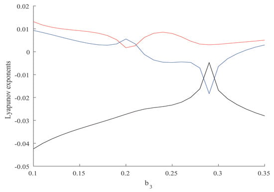
Figure 2.
Lyapunov exponents spectrum.
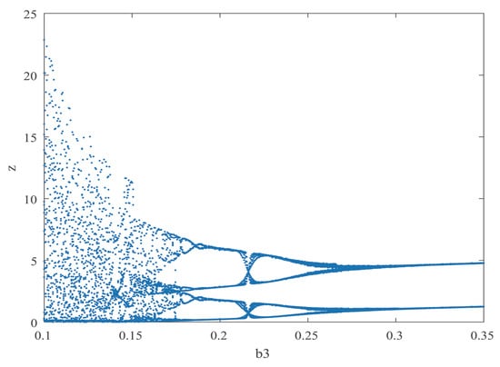
Figure 3.
Bifurcation diagram of z for parameter .
The system has abundant dynamic behaviors according to Figure 2 and Figure 3. Fixing the parameter in the set and the initial value be , we can find a strange attractor as shown in Figure 4a.
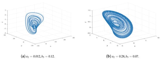
Figure 4.
Two carbon price chaotic attractors. Except for a2 and b3, parameters are the same as a1 = 0.048, a3 = 0.001, b1 = 0.02, b2 = 0.024, c1 = 0.012, c2 = 0.013, c3 = 0.008, L = 1.7, M = 0.9, N = 0.3.
Chaotic behaviors are also observed for parameter set other than . For example, we get a new parameter set by excluding while fixing . Another chaotic attractor (Figure 4b) is observed with the same initial values but . The two attractors have different patterns, indicating various chaotic behaviors of the carbon price system.
4. Case in China: A Stable System
We determine the carbon price system in China using the genetic algorithm method.
4.1. Data Sources and Processing
Data for this study come from the public database and statistical yearbooks. Carbon price data are downloaded from the Carbon Trading Network (http://k.tanjiaoyi.com/). Coal prices of 1500 kcal in Qinhuangdao port are selected as the energy price (http://www.shcce.com/). Data for GDP are obtained from the China Statistical Yearbook 2017. The sample period covers from 2013 to 2017 because that China conducted carbon trading pilot in 2013. We transfer the daily data of carbon price and energy price to annual values by averaging so that their time scales are the same with that of GDP. In detail, the ratio of total transaction price to total transaction volume per year is used as the carbon price data, the annual average of the sum of weekly average prices is used as the energy price data. We first use the carbon price of the Beijing pilot. To be consistent with the carbon price dynamic system, we denote the data of carbon price, energy price, and economic growth as , and respectively. Data of , , as shown in Table 1.

Table 1.
The data of carbon price, energy price, and economic growth.
4.2. Parameter Identification
The identification of parameters is fulfilled by the implementation of the genetic algorithm on the discrete system. The first step is to discretize system (1). We rewrite the carbon price dynamic system in the vector form:
where represents the state of the system, is the system parameter. We next discretize it to
The identifying parameters of the system is equivalent to the nonlinear optimization problem:
Then parameters are identified through the genetic algorithm [42], which is an effective stochastic optimization technique with the characteristics of tiny errors. The algorithm begins with a set of solutions called population. It selects solutions (parents) according to their fitness. New solutions (offspring) are produced either by mutation or by crossover then are placed to be the new population. The algorithm stops when the end condition is satisfied.
This study implements the genetic algorithm in a Matlab 2017 platform with its global optimization toolbox. We normalize the data in Table 1. After repeated attempts, the population size is 200, the crossover rate is 0.5 and the mutation rate is 0.3. When the error tolerance reaches or the number of evolution is 200, the parameters of the example system are obtained and are shown in Table 2.
Table 2.
The parameters of the example system.
We select the data of the year 2013 as the initial conditions, i.e. set initial value as , and choose the parameters in Table 2. The corresponding stable solution could be observed as shown in Figure 5a. Accordingly, the example system is stable, i.e., the example system is sustainable, which meets the real situation. We analyze the phase diagram using the data from Shenzhen Pilot as there are totaly eight carbon pilot markets in China. Following the same procedure for Beijing Pilot, we identify the parameters and find the system is also stable. Figure 5b shows the phase diagram for Shenzhen Pilot. The analogy of the two phase diagrams verifies the structure of the model.
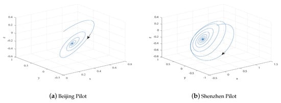
Figure 5.
Phase diagram of the example system.
5. Parameters’ Impact on System Variables
This paper discusses the impact on the carbon price, energy price and economic growth of parameters , , , and . These parameters indicate energy price policy, government control, technological innovation, and the investment to carbon trading, respectively. We conduct three scenario cases by perturbing the parameters. The base case corresponds to using parameters in Table 2, while the strong cases with larger parameters and the weak cases with smaller parameters.
This section first analyzes the impact of energy price policy on the carbon price. Figure 6 shows the evolution curves of the carbon price for three values of . The red lower curve corresponds to the weak case (); the middle blue one, base case (); the upper green one, strong case (). We conclude that carbon price is positively correlated with . Carbon price fluctuates more violently in short terms (). In the long term, it converges as shown in the sub-figure in the right upper corner of Figure 6. This indicates that energy price policy can achieve the purpose of stabilizing carbon price. From the other side, adjusting policies can boost carbon price. However, it takes a long time to reach the stable point. There may also be irreversible impacts on energy and the economy. These findings indicate that appropriate energy price policy should be made and adopted.
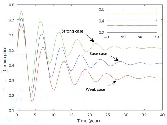
Figure 6.
The evolution tendency of the carbon price for different policy control parameter . Weak case: ; base case: ; strong case: .
The second analysis is the impact of government control on the carbon price. Figure 7 shows the evolution curves of the carbon price for various . The red lower curve corresponds to the weak case (); the middle blue one, base case (); the upper green one, strong case (). Different evolution patterns are observed for the short term () and the long term (). In the short term, the strong case corresponds to a lower carbon price, indicating that a stronger government control inhibits carbon price. However, the negative effects of government control are reversed to positive in the long term. The carbon prices tend to their stable levels. The order of these levels is consistent with that of . This finding shows that government control could promote carbon price to a desired level in the long term although it hinders the price in the short term. Therefore, the government should take an active role in the carbon market, formulating timely adjustable policies to promote the development of carbon trading market.
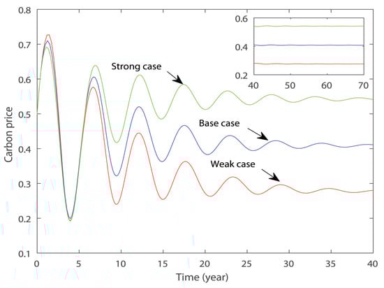
Figure 7.
The evolution tendency of the carbon price for different government control parameter . Weak case: ; base case: ; strong case: .
The third examination is the impact of technical innovation of carbon price on the energy price. Figure 8 shows the evolution curves of energy price for three values of . The red lower curve corresponds to the weak case ( ); the middle blue one, base case (); the upper green one, strong case (). Energy price tends to stable in the long term as the amplitude of the curve decreases. Relative locations of these curves are finally fixed, with the green curve surpasses the red and blue ones, after various exchanging. This indicts that the larger is, the better control effect of the carbon price is. The final evolution results show that technical innovation of carbon price is positively correlated with energy price under the current constraint strength.
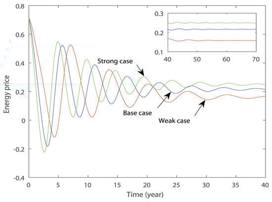
Figure 8.
The evolution tendency of energy price for different technical control parameter . Weak case: ; base case: ; strong case: .
Finally we analyze the impact of the investment to the carbon trading on the economic growth. Figure 9 shows the evolution curves of economic growth for three values of . The upper red curve corresponds to the weak case (); the middle blue one, base case (); the green below one, strong case (). This parameter has an inhibitory effect on economic growth due to the decreasing trend of the curves. The overinvestment to the carbon trading hampers economic development from the fact that all values of economic development are negative in the long run. However, this negative situation could be improved by protecting the carbon market from excessive speculation that can cause unreasonable or unwarranted price fluctuations.
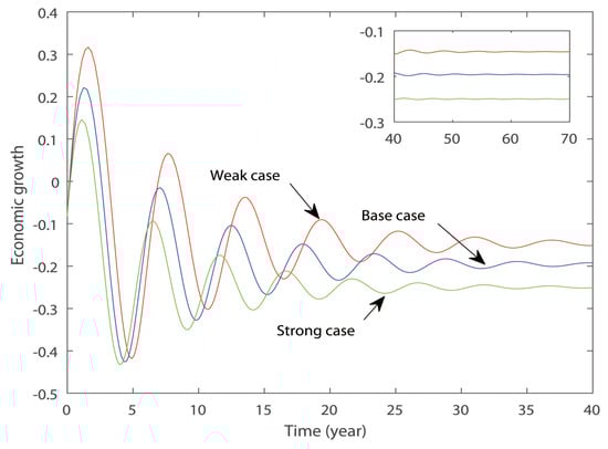
Figure 9.
The evolution tendency of economic growth for different investment control parameter . Weak case: ; base case: ; strong case: .
6. Conclusions
A three-dimensional differential dynamic system is built to describe the interactions among carbon price, energy price, and economic growth. The constructed dynamic system presents complex behaviors. This study finds a possible parameter set for chaos by equilibrium point analysis and dissipative analysis. Under such a parameter set, the system is proved to be chaotic by the Lyapunov exponents spectrum and bifurcation diagram. System parameters in the case of China are identified with the aid of the genetic algorithm. Scenario analysis of the example system is carried out. Impacts of parameters are discussed by analyzing the evolutionary trends of the variables. The hypothesis of complex behavior characteristics is verified through that carbon price can be either chaotic or stable depending on the parameter set.
Results of the evolutionary trends of the carbon price indicate the importance of government control in the carbon market. On the one hand, energy price policy is beneficial to the development of carbon price. On the other hand, the level of the carbon price is negatively related in the short term but positively related to the government control in the long term. This implies that the government can control the carbon price to a level as it desires. Therefore, both policy for energy price and the government control on carbon market should be used cautiously. In addition, appropriate policies should be formulated to function together with government policy. Results show that the technological innovation of carbon price has a positive correlation with energy price. However, the investment in carbon trading is negatively correlated with economic development. The finding implies that a robust carbon market helps to allocate resources reasonably and promote sustainable development.
There are some limitations to this study. Accuracies of the identified parameters may not be perfect due to the limited number of the sample data. While the model is theoretically built, model calibration and validation might be applied to local areas because of the distinct economic background and market environment. The system is valid for countries, particularly underdeveloped countries where fossil energy dominates its energy structure. The model in this paper includes only three variables. However, more variables should be included in the actual emission reduction system, such as public acceptance, economic growth rates. In such a new system, further researches could be carried out on the influences on the carbon price of those new factors. Besides, it is also of interest to study the comparison of system parameters in two or more different countries.
Author Contributions
Conceptualization, X.F. and Y.Z.; Data curation, J.Y.; Methodology, X.F. and J.Y.; Writing—original draft, X.F. and Y.Z.; Writing—review & editing, X.F. and J.Y.
Funding
This research is funded by National Natural Science Foundation of China [Nos. 71673116, 71690242 and 51876081], Natural Science Foundation of Jiangsu Province [No. SBK2015021674] and Humanistic and Social Science Foundation from Ministry of Education of China [No. 16YJAZH007].
Conflicts of Interest
The authors declare no conflict of interest. The founding sponsors had no role in the design of the study; in the collection, analysis, or interpretation of data; in the writing of the manuscript, and in the decision to publish the results.
References
- Zhao, X.; Wu, L.; Li, A. Research on the efficiency of carbon trading market in China. Renew. Sustain. Energy Rev. 2017, 79, 1–8. [Google Scholar] [CrossRef]
- Zhao, X.; Han, M.; Ding, L.; Kang, W. Usefulness of economic and energy data at different frequencies for carbon price forecasting in the EU ETS. Appl. Energy 2018, 216, 132–141. [Google Scholar] [CrossRef]
- Zhang, F.; Fang, H.; Wang, X. Impact of carbon prices on corporate value: The case of China’s thermal listed enterprises. Sustainability 2018, 10, 3328. [Google Scholar] [CrossRef]
- Lutz, B.J.; Pigorsch, U.; Rotfuß, W. Nonlinearity in cap-and-trade systems: The EUA price and its fundamentals. Energy Econ. 2013, 40, 222–232. [Google Scholar] [CrossRef]
- Tan, X.; Wang, X. Dependence changes between the carbon price and its fundamentals: A quantile regression approach. Appl. Energy 2017, 190, 306–325. [Google Scholar] [CrossRef]
- Song, Y.; Liang, D.; Liu, T.; Song, X. How China’s current carbon trading policy affects carbon price? An investigation of the Shanghai emission trading scheme pilot. J. Clean. Prod. 2018, 181, 374–384. [Google Scholar] [CrossRef]
- Yang, B.; Liu, C.; Gou, Z.; Man, J.; Su, Y. How will policies of China’s CO2 ETS affect its carbon price: Evidence from chinese pilot regions. Sustainability 2018, 10, 605. [Google Scholar] [CrossRef]
- Zhang, Y.; Wang, A.; Tan, W. The impact of China’s carbon allowance allocation rules on the product prices and emission reduction behaviors of ETS-covered enterprises. Energy Policy 2015, 86, 176–185. [Google Scholar] [CrossRef]
- Hintermann, B. Allowance price drivers in the first phase of the EU ETS. J. Environ. Econ. Manag. 2010, 59, 43–56. [Google Scholar] [CrossRef]
- Doytch, N.; Uctum, M. Globalization and the environmental impact of sectoral FDI. Econ. Syst. 2016, 40, 582–594. [Google Scholar] [CrossRef]
- Convery, F.J.; Redmond, L. Market and price developments in the European Union emissions trading scheme. Rev. Environ. Econ. Policy 2007, 1, 88–111. [Google Scholar] [CrossRef]
- Kim, M.; Lee, K. Dynamic interactions between carbon and energy prices in the US regional greenhouse gas initiative region. Int. J. Energy Econ. Policy 2015, 5, 494–501. [Google Scholar]
- Zhang, Y.; Sun, Y. The dynamic volatility spillover between European carbon trading market and fossil energy market. J. Clean. Prod. 2016, 112, 2654–2663. [Google Scholar] [CrossRef]
- Kanamura, T. Role of carbon swap trading and energy prices in price correlations and volatilities between carbon markets. Energy Econ. 2016, 54, 204–212. [Google Scholar] [CrossRef]
- Sousa, R.; Aguiarconraria, L.; Soares, M.J. Carbon financial markets: A time–frequency analysis of CO2 prices. Physica A 2014, 414, 118–127. [Google Scholar] [CrossRef]
- Carraro, C.; Favero, A. The economic and financial determinants of carbon prices. Financ. Uver Czech J. Econ. Financ. 2009, 59, 396–409. [Google Scholar]
- Zhang, X.; Xu, Q.; Zhang, F.; Guo, Z.; Rao, R. Exploring shadow prices of carbon emissions at provincial levels in China. Ecol. Indic. 2014, 46, 407–414. [Google Scholar] [CrossRef]
- Zeng, S.; Nan, X.; Liu, C.; Chen, J. The response of the Beijing carbon emissions allowance price (BJC) to macroeconomic and energy price indices. Energy Policy 2017, 106, 111–121. [Google Scholar] [CrossRef]
- Fang, G.; Tian, L.; Liu, M.; Fu, M.; Sun, M. How to optimize the development of carbon trading in China-Enlightenment from evolution rules of the EU carbon price. Appl. Energy 2018, 211, 1039–1049. [Google Scholar] [CrossRef]
- Fan, J.H.; Todorova, N. Dynamics of China’s carbon prices in the pilot trading phase. Appl. Energy 2017, 208, 1452–1467. [Google Scholar] [CrossRef]
- Guo, J.; Su, B.; Yang, G.; Feng, L.; Liu, Y.; Gu, F. How do verified emissions announcements affect the comoves between trading behaviors and carbon prices? Evidence from EU ETS. Sustainability 2018, 10, 3255. [Google Scholar] [CrossRef]
- Chevallier, J. A model of carbon price interactions with macroeconomic and energy dynamics. Energy Econ. 2011, 33, 1295–1312. [Google Scholar] [CrossRef]
- Benz, E.; Trück, S. Modeling the price dynamics of CO2 emission allowances. Energy Econ. 2009, 31, 4–15. [Google Scholar] [CrossRef]
- Daskalakis, G.; Psychoyios, D.; Markellos, R.N. Modeling CO2 emission allowance prices and derivatives: Evidence from the European trading scheme. J. Bank. Financ. 2009, 33, 1230–1241. [Google Scholar] [CrossRef]
- Seifert, J.; Uhrighomburg, M.; Wagner, M. Dynamic behavior of CO2 spot prices. J. Environ. Econ. Manag. 2008, 56, 180–194. [Google Scholar] [CrossRef]
- Fan, X.; Li, S.; Tian, L. Chaotic characteristic identification for carbon price and an multi-layer perceptron network prediction model. Expert Syst. Appl. 2015, 42, 3945–3952. [Google Scholar] [CrossRef]
- Berk, I.; Yetkiner, H. Energy prices and economic growth in the long run: Theory and evidence. Renew. Sustain. Energy Rev. 2014, 36, 228–235. [Google Scholar] [CrossRef]
- Weber, M.; Barth, V.; Hasselmann, K. A multi-actor dynamic integrated assessment model (MADIAM) of induced technological change and sustainable economic growth. Ecol. Econ. 2005, 54, 306–327. [Google Scholar] [CrossRef]
- Fang, G.; Tian, L.; Sun, M.; Fu, M. Analysis and application of a novel three-dimensional energy-saving and emission-reduction dynamic evolution system. Energy 2012, 40, 291–299. [Google Scholar] [CrossRef]
- Fang, G.; Tian, L.; Fu, M.; Sun, M. Government control or low carbon lifestyle?—Analysis and application of a novel selective-constrained energy-saving and emission-reduction dynamic evolution system. Energy Policy 2014, 68, 498–507. [Google Scholar] [CrossRef]
- Fang, G.; Tian, L.; Fu, M.; Sun, M.; Du, R.; Liu, M. Investigating carbon tax pilot in YRD urban agglomerations-Analysis of a novel ESER system with carbon tax constraints and its application. Appl. Energy 2017, 194, 635–647. [Google Scholar] [CrossRef]
- Zhang, G.; Tian, L. Evolution analysis and application of the dynamic system based on energy prices-energy efficiency-economic growth in China. Int. J. Nonlinear Sci. 2017, 23, 109–115. [Google Scholar]
- Wang, M.; Tian, L. Regulating effect of the energy market-Theoretical and empirical analysis based on a novel energy prices-energy supply-economic growth dynamic system. Appl. Energy 2015, 155, 526–546. [Google Scholar] [CrossRef]
- Fan, X.; Xu, H.; Yin, J. Chaotic behavior in a resource-economy-pollution dynamic system. J. Multidiscipl. Eng. Sci. Technol. 2017, 4, 6508–6512. [Google Scholar]
- Hallegatte, S.; Ghil, M.; Dumas, P.; Hourcade, J.C. Business cycles, bifurcations and chaos in a neo-classical model with investment dynamics. J. Econ. Behav. Organ. 2008, 67, 57–77. [Google Scholar] [CrossRef]
- Molz, F.; Faybishenko, B. Increasing evidence for chaotic dynamics in the soil-plant-atmosphere system: A motivation for future research. Procedia Environ. Sci. 2013, 19, 681–690. [Google Scholar] [CrossRef]
- Patten, B.C. Synthesis of chaos and sustainability in a nonstationary linear dynamic model of the American black bear (Ursus americanus Pallas) in the Adirondack Mountains of New York. Ecol. Model. 1997, 100, 11–42. [Google Scholar] [CrossRef]
- Hermanowicz, S.W. Sustainable Development: Physical and Moral Issues; Working Papers; Water Resources Center Archives, University of California Water Resources Center: Berkeley, CA, USA, 2006. [Google Scholar]
- Thomas, C.; Prasad, R.R.; Mathew, M. Introduction to Complex Systems, Sustainability and Innovation. In Complex Systems, Sustainability and Innovation; IntechOpen: London, UK, 2016. [Google Scholar]
- Hudson, C.G.; Vissing, Y.M. Sustainability at the edge of chaos: Its limits and possibilities in public health. BioMed Res. Int. 2013, 2013, 801614. [Google Scholar] [CrossRef]
- Yi, L.; Li, Z.; Yang, L.; Liu, J.; Liu, Y. Comprehensive evaluation on the “maturity” of China’s carbon markets. J. Clean. Prod. 2018, 198, 1336–1344. [Google Scholar] [CrossRef]
- Bastidasrodriguez, J.; Petrone, G.; Ramospaja, C.; Spagnuolo, G. A genetic algorithm for identifying the single diode model parameters of a photovoltaic panel. Math. Comput. Simul. 2017, 131, 38–54. [Google Scholar] [CrossRef]


© 2018 by the authors. Licensee MDPI, Basel, Switzerland. This article is an open access article distributed under the terms and conditions of the Creative Commons Attribution (CC BY) license (http://creativecommons.org/licenses/by/4.0/).