Article

Learning Curve, Change in Industrial Environment, and Dynamics of Production Activities in Unconventional Energy Resources

Department of Energy Resources Engineering, Inha University, 100 Inharo, Nam-gu, Incheon 22212, Korea
*
Author to whom correspondence should be addressed.
Sustainability 2018, 10(9), 3322; https://doi.org/10.3390/su10093322
Submission received: 29 August 2018 / Revised: 14 September 2018 / Accepted: 14 September 2018 / Published: 17 September 2018
(This article belongs to the Section Energy Sustainability)

Abstract

:
Since 2007, shale oil and gas production in the United States has become a significant portion of the global fossil fuel market. The main cause for the increase in production of shale oil and gas in the US is the adoption of new production technologies, namely, horizontal drilling and hydraulic fracturing. However, the production cost of shale oil and gas in the US is comparably higher than the production cost of conventional oil and gas. In 2014, the crude oil and natural gas price decreased significantly to approximately 40 dollars per barrel, and natural gas prices decreased to 3 dollars per million British thermal unit, and thus the productivity and financial conditions for the exploration and production of shale oil and natural gas for producers in the United States have worsened critically. Therefore, technological innovation has become one of the most interesting issues of the energy industry. The present study analyzes the trends in technological innovation having a relationship with production activities. This study calculates the learning rate of 30 companies from the petroleum exploration and production industry in the United States using an improved learning rate calculation formula that reflects the changes in the oil production ratio. Thus, more statistically confident calculation results and interpretations of strategic production activities with regard to changes in the industrial environment were achieved in this study.

1. Introduction

The main focus of the global energy market is the upstream energy industry in the Unites States. Figure 1 shows the crash in the Henry Hub Natural Gas and West Texas Intermediate (WTI) crude oil prices in 2014. The WIT crude oil price decreased from nearly 100 dollars per barrel in late 2014 and continued to decrease to under 40 dollars per barrel in early 2016. The Henry Hub Natural Gas price decreased significantly from nearly five dollars per million British thermal unit in 2014, whereas the natural gas price rebounded in early 2016. Since then, US crude oil prices settled at approximately 50 dollars per barrel between the middle of 2016 to the middle of 2017. Natural gas prices settled and fluctuated at approximately three dollars per million British thermal unit from the middle of 2016. After the crash in commodities prices, price trends have differed. Oil prices increased to 60 dollars per barrel in early 2017. However, natural gas prices have remained at approximately three dollars per million British thermal unit [1,2].
Exploration and production (E&P) companies in the US have persistently suffered during periods of low commodities prices in the past three years. Particular damage has been incurred by E&P companies producing shale gas and tight oil or unconventional petroleum, which have comparatively higher production costs than conventional oil and gas. These players have recorded huge losses while producing oil and gas, which have higher production costs than their commodity prices. From mid-2015 to late 2016, low crude oil and natural gas prices have brought costs down among several US shale E&P players [3]. This decrease in production costs could indicate the beginning of an era of cheap and unconventional oil and gas or could be a temporary change caused by the reduced expenditures of E&P companies. Curtis [4] described the technological development and changes in engineering performance factors related to productivity. Moreover, the results suggest that the discovery of remaining scientific unknowns could possibly improve the productivity of unconventional petroleum-producing technologies.
Gao and You [5] emphasized and suggested improving economic efficiency and sustainability in shale gas production through technological developments throughout the US shale gas industry from upstream to downstream. Middleton et al. [6] showed that technological developments improve production from single wells using fracturing technology. The authors also conducted simulations using data from 20,000 wells from the Barnett formation from 1994 to 2016. Wei et al. [7] analyzed US patent datum and suggested that the technological development of the shale gas industry started from 1966, and patent intensity strengthened from 2005 to 2016. Moreover, they described the most innovative technology in the shale industry, including synthetic carbon oxide, fracture proppant, hydraulic fracturing, and horizontal drilling. Additionally, they highlighted emerging technology in the shale industry, such as model simulations for more precise exploration, fracturing technology in the deep pay-zone, water treatment, and environmental protection technology.
From the perspective of the economics of technology, production cost is a proxy for measuring the magnitude of innovation, and innovation based on technical change reduces the production cost as a result of technological development. A study on technological progress focusing on productivity increases was conducted by Wright in 1936 [8]. The author analyzed the factors inducing a decrease in the production costs of the airplane industry. This prior research on technological development found a productivity gain that occurs according to learned labor skills based on cumulative production. Technological development analyzed according to reputed cumulative production activities have been applied in many ways.
The Boston Consulting Group (BCG) proposed an experience curve model with the same mathematic expression as a learning curve [9]. Furthermore, the BCG suggested that interpretation must be strategic using the experience curve method. In the competitive case, a market leader has the fastest growing productivity in terms of the experience curve and can try to compete to increase their market share by decreasing product prices. In the same manner, other competitive companies will react to competition on the expectations of changes in costs [10].
Cabral [11] provided an explanation of the relationship between price, learning, and cost. The authors showed that predatory pricing strategies to decrease prices and increase market share could decrease production as a result of quicker learning stimulated by competition.
Ibenholt [12] calculated the learning rate for wind power generation and discussed policies for enhancing the learning effect based on competition. The authors also found that R&D funding is as important as technological development in pushing policies. In some cases, if R&D funding does not support enough technological development, production costs can increase. As a recommendation, it is important to promote and suggest a desirable target appropriately.
Dutton and Thomas [13] examined four causal factors capable of affecting the learning rate, and divided the learning phenomenon into autonomous learning and induced learning. The first is technological development in the area of capital goods. In this case, cumulative investment is more important than cumulative production. The second is the Horndal-Plant-effect case. The Horndal-Plant effect refers to an increase in labor productivity through learning. The Horndal-Plant effect also indicates an improvement in the management of inventory, work scheduling, quality control, and wage incentives. The third is the local system characteristics, which are causal factors resulting in the dynamicity of learning in a specific industry. Finally, the fourth is the scale effect, which is a well-known causal factor of learning. The scale effect indicates technological development according to cumulative production, and it is a characteristic of an expanding market and the industrial production scale.
Rapping [14] applied the learning curve concept to production function by adding the cumulative output as a factor in production function. Their results indicate that the cumulative output has a positive relationship with production amount even in models including labor and capital inputs. Kahouli-Bralmi [15] suggested an interpretation explaining the constant return to scale of the learning curve based on the Cobb–Douglas production function.
There have been many applications of the learning curve method in analyzing the technological development of the energy industry. Samadi [16] examined and compared the learning rate of electricity generation technologies using a number of previous studies. Hong et al. [17] calculated the learning rate for photovoltaic power generation in Korea using a two-factor model based on cumulative production and cumulative investment and production costs. They showed that the magnitude of technological development based on investment is higher than technological development through production. Moreover, several studies have examined the learning rate of the upstream petroleum E&P industry. Fukui et al. [18] recently conducted a study regarding technological development and innovation of the upstream energy industry in the US based on production. He analyzed the learning curve of the shale E&P industry in the US using the well-head price and cumulative production.
Kim and Lee [19] calculated the learning rate for shale players in the US using the production cost and drilling count. They compared their results from a traditional one-factor model of 3.08% to a learning rate of approximately 1.89% from 2008 to 2016. Due to the different learning rates, the research period was extended. Moreover, the authors found a meaningful decrease in production costs that was concentrated in the most recent three years. In the prior work, the meaningful period of decrease was just two years, from 2015 to 2016. Kim and Lee [19] found some improvements from the previous study and estimated the learning rate using the production cost and amount of crude oil and natural gas. Moreover, they categorized the learning curve into short and long periods. However, improvements still remain to be achieved through further research. The generally accepted rule of the petroleum E&P industry is to apply the thermal unit cost, barrels of oil equivalent (BOE) per dollar, or the equivalent of a thousand cubic feet of natural gas, integrating multiple petroleum products from a company. However, the actual thermal unit production cost differs between petroleum products.
Thus, this study characterizes the effects of introducing the thermal unit cost of petroleum products into the learning curve method. By adapting an improved empirical method, this study demonstrates an improved statistical confidence level and draws conclusions that describe the causes of innovation from continuously repeated production activities. Moreover, this study provides a deep discussion on technological development, including changes in production activities and industrial environment.

2. Material and Methods

This study is an extension of a previous study [19] and is an attempt to develop a learning curve model with higher statistical accuracy. Thus, this study mainly suggests an improved learning curve method appropriate for application to the upstream of the petroleum production industry. Additionally, this study contains a novel approach for technological progress.

2.1. Learning Curve Method

The learning curve concept originates from a study by Wright [8]. Since then, many studies have been conducted to develop the learning curve method for analyzing the relationships between cumulative production and production cost [9,10,11,12,13,14,15,16,17,18,19,20,21]. This study suggests a new application of the learning curve with a presentation of previous models; the variables used within the models are summarized in Table 1.
The authors characterized the relationship between a decrease in production cost and the production in the airplane industry, which is shown in Equation (1).
C = X n ,
where C is unit cost, X is produced quantity, and n is a factor reflecting variation of unit cost with produced quantity, termed the decline rate. n can be calculated from Equation (2).
n = log C / log X ,
Alchian [20] suggested the learning curve using a statistical approach to introduce a representative form with several alternative progress functions. Through many follow-up studies [9,10,11,12,13,14,15,16,17,18,19,20,21], the mathematical expressions for the learning curve have become generalized [21]
C t   =   C 0 × ( x t x 0 ) L ,
  L R = 1 P R = 1 2 L ,  
Equations (3) and (4) are basic equations used to calculate the learning rate, where L is the learning parameter, C t is the production cost, C 0 is the initial production cost, x t is the cumulative production amount, and x 0 is the initial production. In Equation (3), the traditional form of a learning curve indicates that the production cost can be defined based on the initial production cost and increased cumulative production. In Equation (4), LR is the learning rate and PR is the progress ratio. The learning rate is defined through a multiplier of the cumulative production variable, which means the rate of cost decreases at double the cumulative production amount. The mathematical expressions herein assume that the output from a product is not a mixture of multiple products sharing a particular production technology. However, the upstream petroleum industry produces two representative products, crude oil and natural gas, each having its own substitutability. Thus, the authors suggest a changed form of the learning rate that allows for a consideration of the substitutability of the products of the upstream petroleum industry.
C t   =   C 0 × ( x t x 0 ) L × θ t O ,
  ln C t = ln C 0 L ln X t + O ln θ t ,  
In Equation (5), x t / x 0 also indicates the cumulative production compared to initial production, and θ is the oil production ratio, i.e., the thermal weight of the oil production to the total amount of production. The multiplier O is a dedicated coefficient for the oil production ratio in the natural log transformed equation. In this study, the BOE is adopted as an integrated unit of multiple products. Equation (6) is the natural log transformed expression of Equation (5), which is used in the statistical calculation. In Equation (6), X t represents the cumulative production per initial production ( x t / x 0 ) in Equation (5).
  Y = B 0 + B 1 ln X t + B 2 ln θ t + ε ,  
Equation (7) is a statistical calculation of the learning rate. Here, B 0   is the statistically estimated term for initial cost, B 1 is the learning parameter, and B 2 is the coefficient of the oil production ratio affecting the changes in production cost. B 2 is the multiplier for the oil production ratio in Equation (5). B 2 reflects the effect of the oil production ratio change on production cost and takes a critical role in increasing statistical accuracy and can be obtained through the statistical calculations. Therefore, the learning rate from the proposed model, Equation (5), can be different from the traditional learning rate model, Equation (3), by adding the oil production ratio.

2.2. Data Collection

Data were collected from an annual report on 30 companies publishing their individual annual financial reports through the Security Exchange Commission of the United States [22]. In particular, they were selected as samples of independent E&P companies producing shale oil and tight gas in the United States. The production costs include the operating costs, production tax, depletion, depreciation, and amortization costs; general and administrative; and transportation and processing costs. Moreover, production data were also collected from an annual report, which include the amount of oil production in barrels of oil, the amount of gas production in cubic feet, and the entire production in barrels of oil equivalent.

3. Results and Discussion

For an insightful discussion regarding the calculation results, descriptive interpretations of the market and industrial changes during the survey period are needed.

3.1. Calculation of Learning Rate

In this study, several calculations were conducted to identify the learning rate for companies and the industry based on financial and production data from the 30 companies. The specific calculation results based on Equations (1) and (3) are summarized in Table 2.
The learning rate for the traditional one-factor model is 3.086%, with an R-squared value of 0.0181 and an F-statistics probability of 0.0198. However, the R-squared value for the traditional one-factor model is very low.
In Table 2, the model proposed results in a learning rate of 3.989%, with an R-squared value of 0.5626 and an F-statistics probability very close to zero. The coefficient of the oil production ratio from the proposed model has a positive value, which is in contrast to the learning parameter. This implies that the oil production cost is higher than the natural gas production cost. Producers can change the product ratio between crude oil and natural gas, and changes in the product ratio could impact the production costs of the company.
The proposed model results in a learning rate that is 0.903% higher than that of a traditional one-factor model. Critically, a large difference in statistical accuracy is shown. The R-squared value of the proposed model is 0.5445 higher than that of the traditional one-factor model. This impressive improvement may have been derived from the cost increase factor.
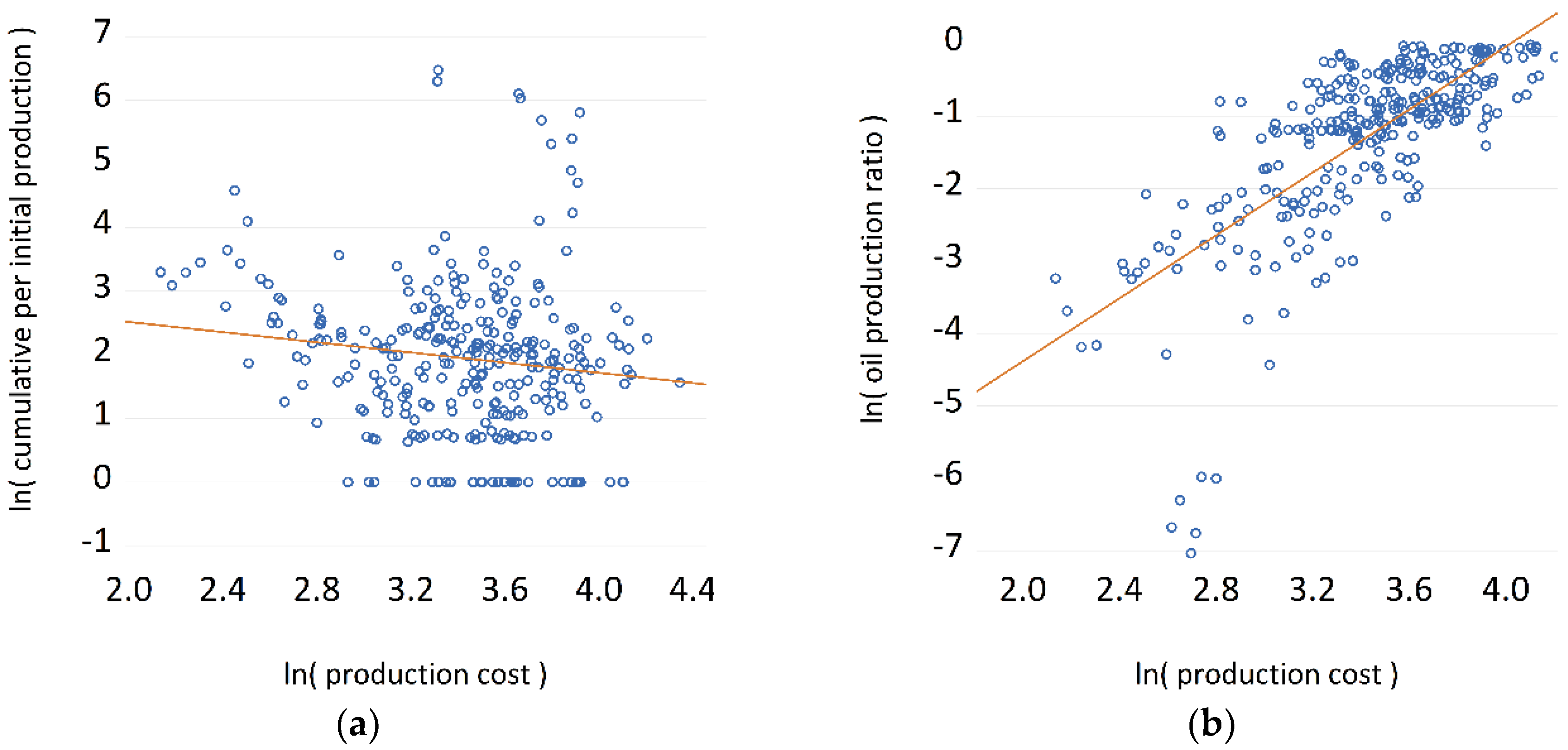
As shown in Table 3, the correlation value between production cost and cumulative production per initial production is −0.0642, and the correlation value between production cost and the oil production ratio is 0.3491. The absolute difference between these two correlation values is 0.2849. The probability coefficient for the production cost with the oil production ratio is 0.0198 smaller than the probability coefficient for the cumulative production per initial production with a full cost.
Moreover, as shown in Figure 2, the correlation between the production cost and the oil production ratio is more concentrated and intensive. It also appears to be more accurate than the correlation between the production cost and the cumulative production per initial production.
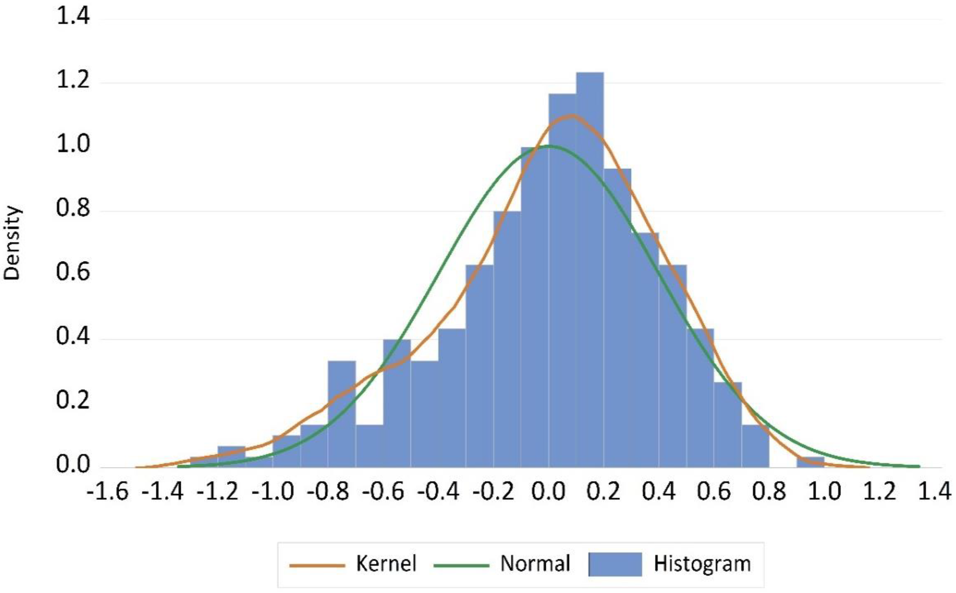
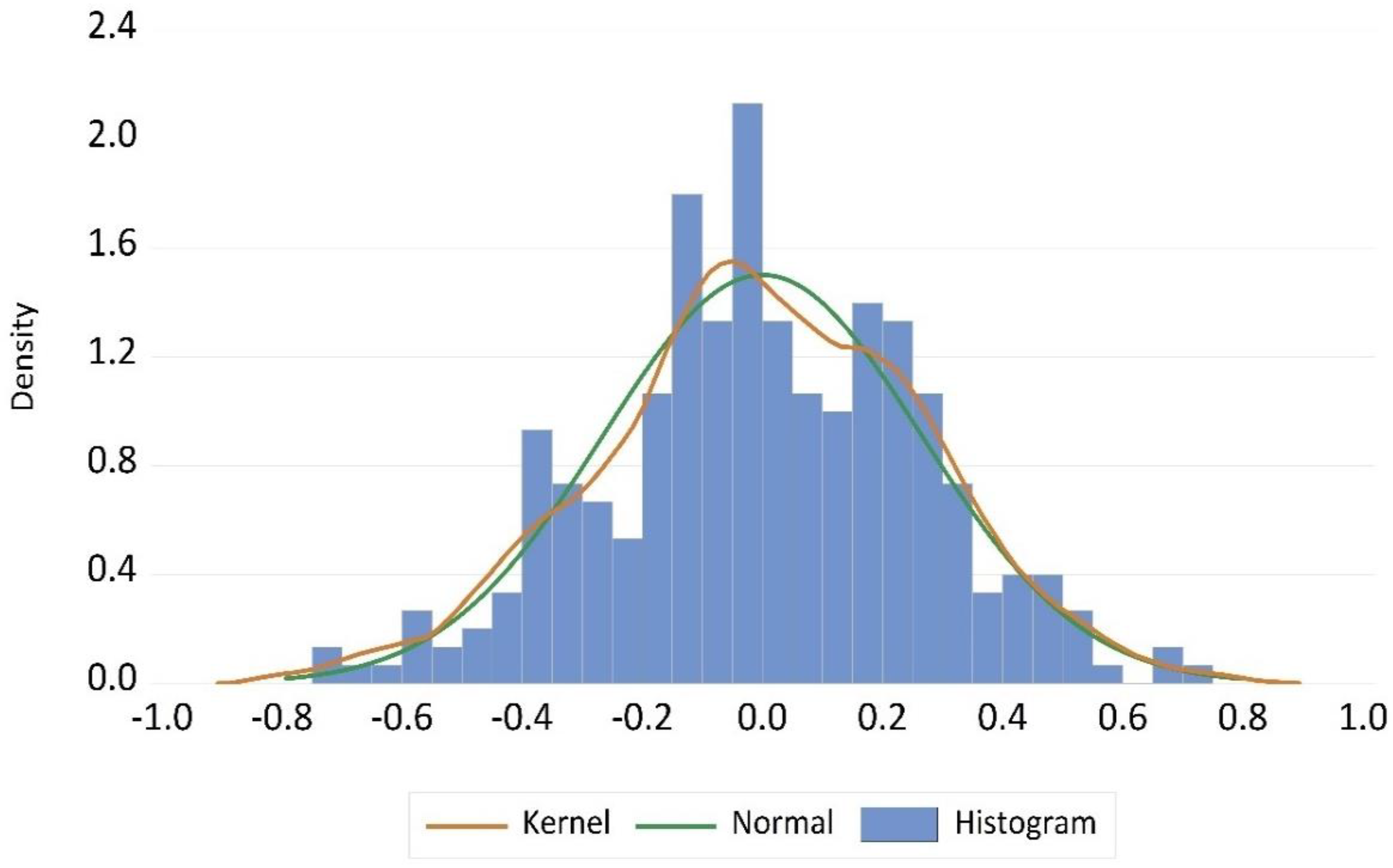
Additionally, the residual distribution of the proposed model appears to be more similar to a normal distribution, as shown in Figure 3 and Figure 4.
As shown in Table 4, the median and mean values of the residual distribution from the proposed model are closer to zero.

3.2. Discussion of Technological Development, Changes in Market Environment, and Production Activities for the 30 E&P Players

To summarize the changes in the Henry Hub Natural Gas and WTI crude oil prices for the last 10 years, the commodities prices crashed in 2008 and 2014. Henry Hub natural gas and WTI crude oil prices were decoupled in 2010 compared to the WTI crude oil price, which increased to nearly 100 dollars per barrel, and high oil prices continued until late 2014. In contrast, the Henry Hub Natural Gas price fluctuated at approximately four dollars per million British thermal unit from 2009 to 2014.
The commodities price crash was induced by OPEC predation, i.e., predatorial action with price declines to compete with rival companies [11]. This action is also termed a squeezing strategy [23]. BCG’s [10] experience curve model includes several competitive applications such as predation. In some cases in the US, the price change occurs in two phases. First, the price continues at the pre-existing level. Second, the price suddenly decreases. These two phenomena are the result of strategic corporate competition, which results in a temporary increase in productivity to survive the competition. Cabral [11] suggested that the positive side of cost competition is that companies learn to develop their productivity when they are under pressure from price decreases.
As shown in Figure 5, the changes in production costs from 30 companies were similar to those in commodities prices. However, in 2017, they did not increase but rather decreased compared to the previous year. This phenomenon was due to an increase in operating costs and production taxes according to an increase in production. The Energy Information Administration of the United States pointed out that an increase in production costs from upstream companies was based on an increase in cost factors according to a greater need for production facilities, tools, and equipment [24]. In a predation case, increases in production cost could cause company closure because some companies fail to successively increase productivity [11]. However, some upstream companies successfully achieve higher productivity based on technological development [4,5,6,7]. This has resulted in a change in productivity and oil production ratio in recent years.
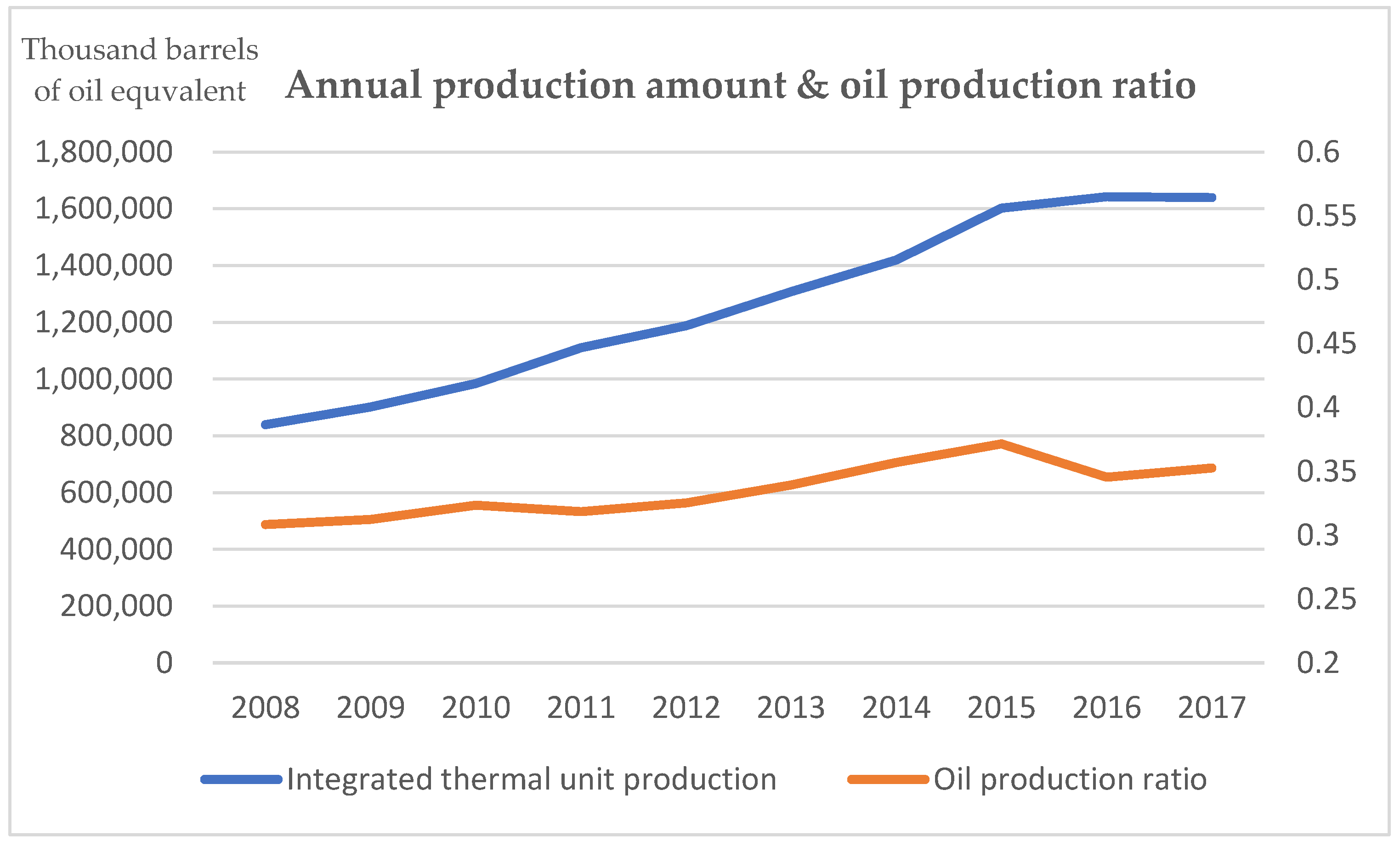
While high oil prices were sustained, annual production increased, and the oil production ratio rapidly increased from 2011 to 2014, as shown in Figure 6.
In 2014, oil and natural gas prices crashed and were recoupled. From 2015 to early 2017, WTI oil prices were under 60 dollars per barrel, and the Henry Hub Natural Gas price remained at approximately three dollars per British thermal unit. While the commodities prices were recoupled, annual production increased, whereas the oil production ratio slightly decreased, from 2014 to 2016. In 2017, the oil production ratio slightly increased, but it was still below the oil production ratio in 2015. In addition, there may have been another reason for the increase in proportion of gas production. Some studies have shown that the reason for an increase in global gas dependency on energy use has been due to environmental concerns and the production of shale oil and gas [25].
Recently, there have been opposing expectations and interpretations on the issue of decreasing production costs for shale oil and gas producers [3]. First, the decrease in the production cost of shale oil and gas will not continue because the decrease in production costs depends on a cut in service costs, and there are almost no technological developments to decrease production costs. Second, the positive expectation on productivity gain means that a decrease in production costs will continue or a decrease in production costs will be sustained in the future because some technological developments will occur to increase efficiencies [4,6,7].
Moreover, some studies on learning rate have suggested that the increase in the unit production scale will have a simultaneous learning effect. The BCG [10] suggested that the change in scale occurs simultaneously with total experience, i.e., the change in scale affects the increase in efficiency and productivity. Ibenholt [12] argued that an increase in unit production scale is characteristic of successful learning. Moreover, the authors emphasized appropriate goals in developing learning technology.
Recent studies have shown that technological development enhances profitability, such as design optimization, which suggests that the US upstream industry is finding appropriate technological development goals [5,26]. Curtis [3,4] showed the technological development of the shale oil and gas upstream industry by presenting engineering factors, including the estimate of ultimate recovery (EUR) and increases in single-well production from decline curve analysis. In other words, recent technological changes in the shale oil and gas upstream industry show that the increase in the production scale of a single well or rig results in an increase in productivity from the shale oil & gas upstream industry. Moreover, recent innovation activities of the US petroleum upstream industry have focused on productivity gains [7].

4. Conclusions

The upstream petroleum industry in the United States has started to produce shale gas and tight oil at high production costs. In 2014, the commodities prices crashed, and technological development became one of the most interesting issues of the global energy market. To consider the technological development that took place after this crash in commodities prices, the learning rate for 30 upstream companies producing shale oil and tight gas in the US was calculated in this study. The results show that proposed model achieves a learning rate of 3.989%, whereas the learning rate from a traditional one-factor model is 3.086%. This difference is derived from the factors that are considered to increase production costs. From 2011 to 2014, the oil production ratio increased, as did the production costs. However, after 2015, the oil production ratio and production costs decreased despite an increase in annual production. This contrasting production trend compared to the production trend prior to the commodities price crash indicates that unconventional production companies in the United States increased their productivity by changing the portion of their shared petroleum production technologies and achieved substitutability.
Additionally, this study suggests a new formula for calculating the learning rate. The actual production costs of products in certain industries can fluctuate according to environmental changes in the market, as seen in the case of upstream industries in the United States. As a result, a high statistical accuracy was achieved in this study for calculating the learning rate by adding the cost-increasing factors.
This study refers to some recent technological developments in the introduction and discussion. These technological developments are not coincidental, but a result of innovative activities such as investment. Even with improved statistical accuracy, this study has limitations; it does not cover innovative activities that could induce technological development. Therefore, further research is required to measure the effect of innovation activities on productivity gains or technological developments.

Author Contributions

Conceptualization, J.-H.K. and Y.-G.L.; Methodology, J.-H.K. and Y.-G.L.; Software, J.-H.K.; Validation, J.-H.K. and Y.-G.L.; Formal Analysis, J.-H.K. and Y.-G.L.; Investigation, J.-H.K. and Y.-G.L.; Resources, J.-H.K. and Y.-G.L.; Data Curation, J.-H.K.; Writing-Original Draft Preparation, J.-H.K.; Writing-Review & Editing, Y.-G.L.; Visualization, J.-H.K.; Supervision, Y.-G.L.; Project Administration, Y.-G.L.; Funding Acquisition, Y.-G.L.

Funding

This study was funded by Inha University.

Conflicts of Interest

The authors declare no conflict of interest. The funder had no role in the design of the study; in the collection, analyses, or interpretation of data; in the writing of the manuscript, and in the decision to publish the results.

References

  1. Cushing, O.K. WTI Spot Price FOB (Dollars per Barrel). Available online: http://tonto.eia.gov/dnav/pet/hist/LeafHandler.ashx?n=PET&s=RWTC&f=M (accessed on 2 July 2018).
  2. Henry Hub Natural Gas Spot Price (Dollars per Million Btu). Available online: http://tonto.eia.gov/dnav/ng/hist/rngwhhdm.htm (accessed on 2 July 2018).
  3. Curtis, T. Unravelling the US Shale Productivity Gains; Oxford Institute for Energy Studies: Oxford, UK, 2016. [Google Scholar]
  4. Curtis, T. Completion Design Changes and the Impact on US Shale Well Productivity; Oxford Institute for Energy Studies: Oxford, UK, 2017. [Google Scholar]
  5. Gao, J.; You, F. Design and optimization of shale gas energy systems: Overview, research challenges, and future directions. Comput. Chem. Eng. 2017, 106, 699–718. [Google Scholar] [CrossRef]
  6. Middleton, R.S.; Gupta, R.; Hyman, J.D.; Viswanathan, H.S. The shale gas revolution: Barriers, sustainability, and emerging opportunities. Appl. Energy 2017, 199, 88–95. [Google Scholar] [CrossRef]
  7. Wei, Y.; Kang, J.; Yu, B.; Liao, H.; Du, Y. A dynamic forward-citation full path model for technology monitoring: An empirical study from shale gas industry. Appl. Energy 2017, 205, 769–780. [Google Scholar] [CrossRef]
  8. Wright, T.P. Factors affecting the cost of airplanes. J. Aeronaut. Sci. 1936, 3, 122–128. [Google Scholar] [CrossRef]
  9. Boston Consulting Group (BCG). Perspectives on Experience; Boston Consulting Group: Boston, MA, USA, 1970. [Google Scholar]
  10. Bosch Franciscus, A.; van den Porter, M.E. Perspectives on Strategy. Boston Consulting Group; Kluwer Academic Publisher: Dordrecht, The Netherlands, 1997. [Google Scholar]
  11. Cabral, L.M.B. The learning curve, market dominance, and predatory pricing. Econometrica 1994, 62, 1115–1140. [Google Scholar] [CrossRef]
  12. Ibenholt, K. Explaining learning curves for wind power. Energy Policy 2002, 30, 1181–1189. [Google Scholar] [CrossRef]
  13. Dutton, J.M.; Thomas, A. Treating Progress Functions as a Managerial Opportunity. Acad. Manag. Rev. 1984, 9, 235–247. [Google Scholar] [CrossRef]
  14. Rapping, L. Learning and World War II Production Functions. Rev. Econ. Stat. 1965, 47, 81–86. [Google Scholar] [CrossRef]
  15. Kahouli-Brahmi, S. Technological learning in energy–environment–economy modelling: A survey. Energy Policy 2008, 36, 138–162. [Google Scholar] [CrossRef]
  16. Samadi, S. The experience curve theory and its application in the field of electricity generation technologies—A literature review. Renew. Sustain. Energy Rev. 2018, 82, 2346–2364. [Google Scholar] [CrossRef]
  17. Hong, S.; Chung, Y.; Woo, C. Scenario analysis for estimating the learning rate of photovoltaic power generation based on learning curve theory in South Korea. Energy 2015, 79, 80–89. [Google Scholar] [CrossRef]
  18. Fukui, R.; Greenfield, C.; Pogue, K.; van der Zwaan, B. Experience curve for natural gas production by hydraulic fracturing. Energy Policy 2017, 105, 263–268. [Google Scholar] [CrossRef]
  19. Kim, J.H.; Lee, Y.G. Analyzing the Learning Path of US Shale Players by Using the Learning Curve Method. Sustainability 2017, 9, 2232. [Google Scholar] [CrossRef]
  20. Alchian, A.A. Reliability of progress curves in airframe production. Econometrica 1963, 31, 679–693. [Google Scholar] [CrossRef]
  21. Yelle, L.E. The learning curve: Historical review and comprehensive survey. Decis. Sci. 1979, 10, 302–328. [Google Scholar] [CrossRef]
  22. Companies Financial Fillings of The United States. Available online: https://www.sec.gov/edgar/searchedgar/companysearch.html (accessed on 2 July 2018).
  23. Behar, A.; Ritz, R. An Analysis of OPEC’s Strategic Actions, US Shale Growth and the 2014 Oil Price Crash; IMF Working Paper; International Monetary Fund: Washington, DC, USA, 2016. [Google Scholar]
  24. Energy Monitor Worldwide. Trends in U.S. Oil and Natural Gas Upstream Costs; Energy Monitor Worldwide: Amman, Jordan, 2016. [Google Scholar]
  25. Turk, J.K.; Reay, D.S.; Haszeldine, R.S. Gas-fired power in the UK: Bridging supply gaps and implications of domestic shale gas exploitation for UK climate change targets. Sci. Total Environ. 2018, 616, 318–325. [Google Scholar] [CrossRef] [PubMed]
  26. Saussay, A. Can the US shale revolution be duplicated in continental Europe? An economic analysis of European shale gas resources. Energy Econ. 2018, 69, 295–306. [Google Scholar] [CrossRef] [Green Version]
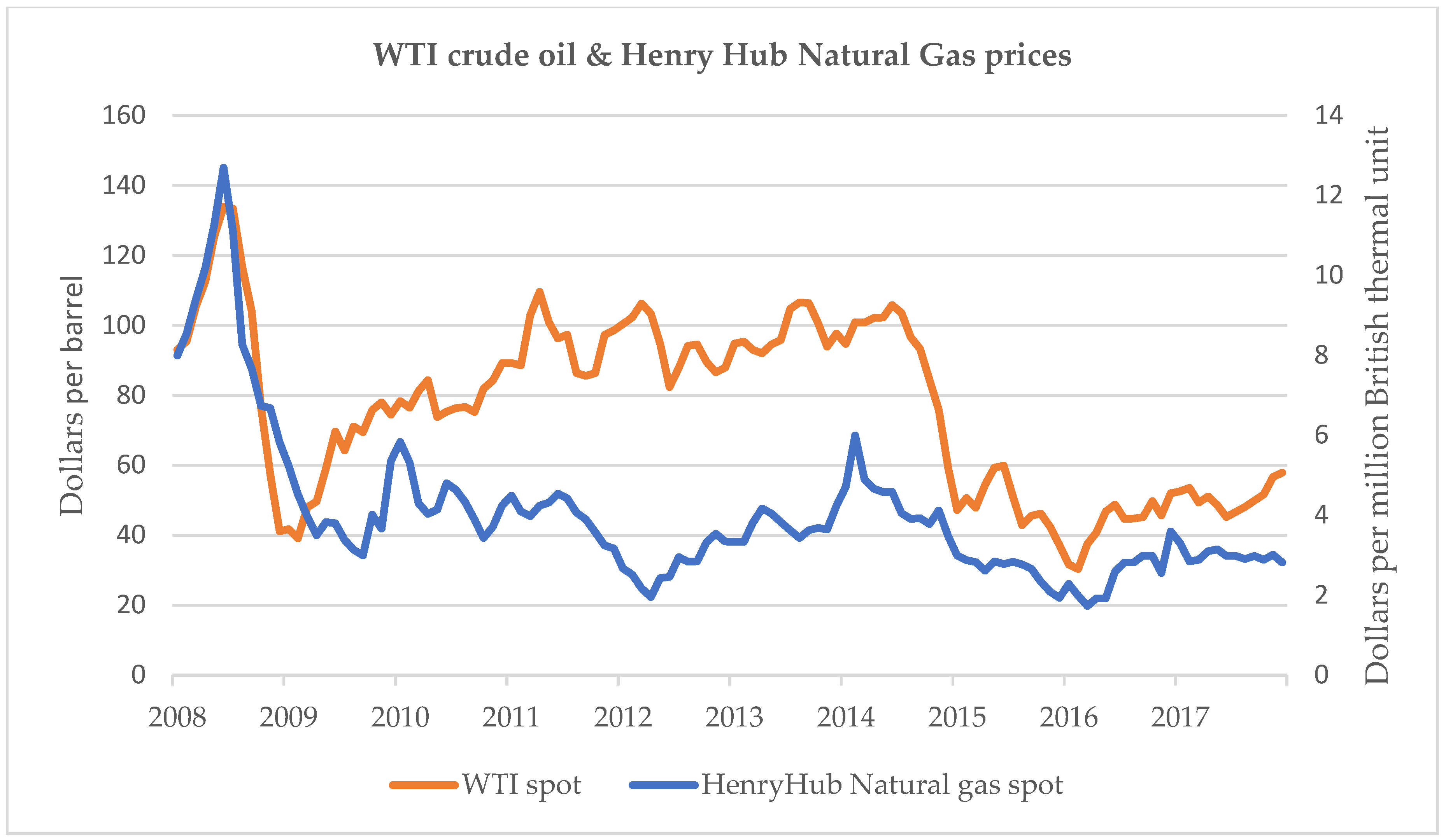
Figure 1. Natural gas and crude oil price changes from 2007 to 2018. WTI: West Texas Intermediate.
Sustainability 10 03322 g001
Figure 2. Correlation between production costs with (a) cumulative production per initial production and (b) oil production ratio.
Sustainability 10 03322 g002
Figure 3. Residual distribution from the traditional one-factor model.
Sustainability 10 03322 g003
Figure 4. Residual distribution from the proposed model.
Sustainability 10 03322 g004
Figure 5. Changes in production costs and detailed description of composites.
Sustainability 10 03322 g005
Figure 6. Changes in annual petroleum production and oil production ratios for 30 companies in the upstream petroleum industry in the Unites States from 2008 to 2018.
Sustainability 10 03322 g006
Table 1. Summary of variables used in the equations.
Formula (1)CXn
Unit costProduced quantityDecline rate
Formula (3) C t C 0 x t x 0 L
Unit costInitial unit costCumulative productionInitial productionLearning parameter
Formula (4) L R PR
Learning rateProgress rate
Formula (6) θ O
Oil production ratioCoefficient of oil production ratio
Table 2. Calculation of learning rate and comparison of models.
Traditional One-Factor Model, Equation (1)
B0B1 Learning RateR2Adjusted R2
Value3.5115−0.0452 3.086%0.0180.0148
Probabilityless than 0.0000.0198 0.01977 (F-statistic)
Proposed Model,Equation (3)
B0B1B2Learning RateR2Adjusted R2
Value3.8575−0.05870.24803.989%0.56260.5597
Probabilityless than 0.000less than 0.000less than 0.000less than 0.000 (F-statistic)
Differences between the Traditional One-Factor Model and Proposed Model,Equations (1)–(3)
B0B1 Learning RateR2Adjusted R2
Value0.34604−0.0135 0.903%0.54450.5449
Probabilityless than 0.000−0.0198 0.0198 (F-statistic)
Table 3. Correlation values of production costs with cumulative production per initial production and oil production ratio.
Cumulative Production Per Initial Production, ln ( x t / x 0 ) Oil Production Ratio, ln ( θ )
Value−0.06420.3491
Probability0.0198less than 0.000
Table 4. Characteristics of the residual distributions from the two models.
MeanMedianStandard DeviationSkewnessKurtosis
Traditional one-factor model1.06 × 10−150.04630.3976−0.54503.0986
Model proposed in this study3.72 × 10−16−0.01810.2655−0.11282.9018