Study on the Selection Strategy of Supply Chain Financing Modes Based on the Retailer’s Trade Grade

Abstract

In the supply chain financing (SCF) system composed of a capital-constrained retailer, a supplier and a commercial bank, we design two different limited financing modes (internal financing and external financing) based on the retailer’s collateral assets. A newsvendor-like retailer has a single opportunity to order goods from a supplier to satisfy future uncertain demand. In the presence of bankruptcy risk for the retailer, we model their strategic interaction as a Stackelberg game with the supplier as the leader and analyze the optimal decisions for each participant. Regardless of which financing mode is chosen, the capital-constrained retailer orders fewer goods if the financing cost is relatively high. In addition, when the market demand obeys the uniform distribution, if the retailer possesses more collateral assets, he will enjoy a lower loan interest rate and increase order quantity gradually. Moreover, compared with the internal financing mode, each participant obtains the larger expected profits under the external financing mode.

1. Introduction

In recent years, financing difficulties have been obsessed with small and medium enterprises (SMEs) [1]. A lack of capital restricts production and purchase decisions made by a company [2]. The study of Archibald has proved that it is difficult for small companies to survive if they are not able to raise funds what they need [3]. This issue can be addressed if SMEs get financing service, so the new value will be created in the supply chain [2]. Therefore, short-term financing is necessary for them to finish their procurement actions, as it does have a positive impact on a firm’s capability to adopt sustainable supply chain management practices [4].

However, many studies [5,6,7] have shown shortcomings of SMEs including information asymmetries, and imperfect financial policies may lead to financing difficulties. Fortunately, there are also several ways to solve their financing problems. For example, although SMEs have been disadvantaged by lack of credit history, they might try to use the fixed asset to mortgage. Some studies have proved that obtaining collateral loan is a feasible way [8,9,10,11,12], especially when the leader enterprise is willing to provide SMEs a guarantee. It is unavoidable that there exist supply chain effects of bankruptcy, but the leader enterprise is encouraged to help other members to obtain enough loans in order to remain superiority as well as improving supply chain efficiency [13,14]. Hence, internal financing has become the prevailing short-term financing mode for the retailer, even for environments with quit well-developed financial markets, such as the United States, when the supplier has adequate money [15].

As a matter of fact, fixed assets are those assets that are used by enterprises for a long time. These assets are earning assets and provide the basis for the firm’s earning power and value [16]. It is not only used to mortgage but also to measure the enterprise’s trade grade. Generally speaking, the greater value of fixed asset represents the higher grade. Based on this, the prevalence of SCF (Supply Chain Financing) brings the several forefront research questions: whether the enterprise with more collateral assets deserves better items (e.g., lower lending rates from banks or suppliers)? How SMEs choose the financing mode based on their own asset value to achieve the maximum profit? Whether the leader enterprise is worth guaranteeing for the follower?

In this paper, we address these questions by designing two different financing modes and making comparisons between them from the point of view of ordering decision to explore which mode is more suitable to the retailer. In this supply chain, a supplier sells goods to a newsvendor retailer facing uncertain demand. The end-product demand distribution and retail price are exogenously specified. The supplier and retailer are risk-neutral profit maximizers. Meanwhile, only the retailer might be capital-constrained, and when in need, he can borrow from a bank with a guarantee of the core supplier or the supplier himself. Each party makes decisions about their decision variables separately.

Our work contributes to the literature in three ways. First, we firstly introduce fixed assets and utilize it to measure the retailer trade grade in the real business environment, though it cannot be used to purchase goods. Second, we formulate the external financing mode under the supplier buy-back contract guarantee and correct the bankruptcy risk because of ignorance and simplification of models in previous studies. Moreover, we compare different financing modes and clarify the higher trade grade of the retailer deserves the better item.

The remainder of the article is organized as follows. Section 2 introduces the related literature. In Section 3, we introduce a modeling framework of SCF which includes problem description, notations, and assumptions. Section 4 formulates a Stackelberg game of SCF and analyzes the optimal decisions for each participant. In Section 5, we numerically compare optimal decisions between different financing modes and explore the impacts of the retailer’s collateral assets on operational decisions through comparative analysis. Finally, Section 6 concludes with remarks.

2. Literature Review

In recent years, SCF has increasingly received substantial interests among supply chain practices and academic fields [17,18,19,20]. Basing on a broad literature, our work aims to examine whether the retailer’s fixed asset influence the lending rate or not in different financing modes (internal financing and external financing), give operational decisions of each participant as well as compare the supply chain performance of two different modes.

On the one hand, some scholars have studied internal financing (supplier financing) in the capital-constrained supply chain, which refers to an agreement between a retailer and a supplier where the latter allows the former to delay payment under given conditions [21]. According to the study of Fisman and Raturi [22], suppliers are willing to provide internal financing with their customers in order to occupy a larger market share even if they encounter financial constraints. Yang and Birge show supply chain efficiency can be improved when a distressed firm receives financing from its supplier [23]. Federgruen and Wang examine different supplier financing mechanisms in a multi-period supply chain model [24].

On the other hand, external financing (bank financing) is also likely to be a mode of short-term financing [25,26,27], showing that the main method to solve the cash constraint problem is asking for a loan from the bank. The first attempt to incorporate asset-based financing into production decisions is reported by Buzacott and Zhang [9]. They research the integration of logistics and cash-flow and build a strategy between a bank and a retailer under uncertain demand, combining financing decisions based on assets and production inventory decisions. By pledging their movable assets, such as raw materials and products, to banks as security, the retailer is able to borrow funds from banks, from which they could not borrow in a conventional loaning system [4]. Chen et al. find that banking financial creates new value in the supply chain, including promoting the rivalry of financial markets as well as affecting the decision-making of the supply chain [28].

Of course, there are some scholars who focus on the comparison of different financing modes. Caldentey and Chen investigate the role of financial service in a procurement contract with a budget-constrained retailer. They concern about the internal financing of supplier’s trade credit and external financing of bank loans, in which the lending bank makes zero profit in a competitive financial market [29]. In a condition that both the supplier and the retailer face capital constraints, the trade credit is more effective than the real contract when they apply for financing from financial institutions [19].

Although extensive work has been done to address issues of optimal strategies in SCF, very little attention has been paid to the retailer’s bankruptcy, or they simply think the retailer will go bankrupt if he is not able to afford a loan, which mismatches the real situation. Bankruptcy is a critical business decision, in which firms declare their inabilities to meet their financial obligations and obtain protection from creditors [14]. Economists have also studied the supplier’s role when facing a buyer with bankruptcy risk. Wilner argues that trade creditors may be willing to grant more concessions when the debtor is in financial distress. Scholars in law and economics have provided in-depth analyses of different bankruptcy rules that affect firm operations [30]. Baird and Picker [31], Bebchuk and Chang [32], and Kordana and Posner [33] design different game-theoretical models to capture the bargaining process of different shareholders in the bankruptcy process and examine various rules in the United States. Considering the real bankruptcy risks, we extend our research by designing two different financing modes that take bankruptcy risks of the retailer into account. The most closely related paper is Kouvelis and Zhao, which presents a trade credit model to study the interaction of short-term financing and inventory decisions and makes comparisons between trade credit and bank financing [34]. While some of our analysis is similar to results in [34], the key distinction is that we formally design external financing mode, which the retailer can raise found under the guaranteeing contract of the core supplier.

The fact is that the supplier often uses the buy-back as a guarantee to reduce the risk of the failure in repayment punctually, which assists the retailer to share risk and improve performance. Padmanabhan designs return policies to enable the retailer to mitigate risks and help the supplier protect product brands [35], which occurs frequently in the real trend. Some studies also show that the buy-back contract, an important supply chain contract, can significantly improve the overall efficiency of the supply chain [36,37,38]. Wang et al. consider not only the bankruptcy risk, but also the situation that the manufacturer buys back a certain percentage of unsold products and the retailer takes the acceptance draft as a settlement tool for finance products [39]. Although both of studies consider about the retailer’s bankruptcy risk, our work still differs from their works, the biggest difference lies in the fact that we focus on researching the internal, external financing simultaneously and compare differences of two modes instead of financing through confirming warehouse system.

3. Modeling Framework of Supply Chain Financing

In this section, we set up a stylized single-period newsvendor model of the SCF system, involving three parties: a capital-constrained retailer, an upstream supplier, and a commercial bank. Firstly, we introduce the problem description; then, we list the model notations and assumptions.

3.1. Problem Description

To clearly describe and analyze our quantitative models, we firstly show the internal and external frameworks in Figure 1 and Figure 2, respectively.

In our model, the retailer faces a situation equivalent to the classical newsvendor problem, where he purchases single goods from the supplier and then sells them to his customers, not knowing the actual market demand for products at the time of purchase. The retailer’s initial procurement capital is $\mathrm{y}$. Noting that $\mathsf{\omega }$ and $\mathrm{p}$ are the terms representing the wholesale price and the market price, respectively. Since the product market and the wholesale market are perfectly competitive, $\mathsf{\omega }$ and $\mathrm{p}$ remain unchanged. When the retailer’s initial capital cannot afford the order, there are two financing modes.

One way is that the retailer can choose to order $\mathrm{q}$ from the supplier and pay $\mathrm{y}$ firstly at the beginning based on collateral assets $\mathrm{Z}$. The remaining part $\left(\mathsf{\omega }\mathrm{q}-\mathrm{y}\right)(1+{\mathrm{r}}_{\mathrm{s}}$) will be repaid after the end-of-season sale. If the retailer falls through, the supplier will obtain the retailer’s total revenue, collateral assets and undertake the remaining loss.

Another way is that the retailer, who is under the guarantee of the supplier’s buy-back contract, uses collateral assets $\mathrm{Z}$ to loan $\left(\mathsf{\omega }\mathrm{q}-\mathrm{y}\right)$ from the bank, and at the end-of-season sale, the retailer repays the loan obligation $\left(\mathsf{\omega }\mathrm{q}-\mathrm{y}\right)\left(1+{\mathrm{r}}_{\mathrm{b}}\right)$ to the bank if the market prospect is bright. When the retailer has the rest of products, the supplier will buy them back at the price $b$. When the retailer goes bankrupt, the bank will receive all sales revenue, collateral assets, and buy-back funds.

The retailer’s trade grade is mainly measured by the collateral assets $\mathrm{Z}$. The more collateral assets represent the retailer’s trade grade is higher. The uncertain demand is denoted by a random variable, $\mathrm{x}\in \left[0,+\infty \right)$. The probability density function (PDF) of $\mathrm{x}$ is $f\left(\mathrm{x}\right)$, the cumulative distribution function (CDF) is $F\left(\mathrm{x}\right)$, and complementary CDF is $\overline{F}\left(\mathrm{x}\right)$($\overline{F}\left(\mathrm{x}\right)=1-F\left(\mathrm{x}\right)$), where we assume $f\left(\mathrm{x}\right)>0$ when $\mathrm{x}>0$.

3.2. Notation and Assumption

As with the usual assumptions of these studies [34,39,40,41], our modeling assumptions are shown as following:

(1)

Information is symmetrical among the supplier, retailer as well as the bank. All of them are risk-neutral and pursue the maximization of profits.

(2)

The bank and the supplier are assumed to face no bankruptcy risk; the retailer may face bankruptcy risk, depending on whether his liquid assets and collateral assets can cover his loan obligations.

(3)

The retailer is credit-worthy and will repay their loan obligations (if any) to the extent possible.

(4)

Goodwill cost is ignored in our model.

(5)

To ensure that the model has an optimal solution, we assume that the demand distribution function $F\left(\mathrm{x}\right)$ is continuous, steerable, and strictly increasing. We restrict our attention to demand distributions with an increasing failure rate (IFR).

(6)

Note that if $\omega \left(1+{\mathrm{r}}_{\mathrm{i}}\right)>p$, the retailer does not order, and if $\omega$ < c, the supplier is not willing to sale. To avoid trivial cases, we assume $p>\omega \left(1+{\mathrm{r}}_{\mathrm{i}}\right)>c$.

The main symbols used in this paper are shown in

Table 1. Notation.

$\mathrm{Z}$: Retailer’s collateral assets pledged to secure the loan.

$\mathrm{y}$: Retailer’s initial capital when purchasing

$\mathrm{P}$: Retailer’s unit retail price of the product

$\mathsf{\omega }$: Supplier’s unit wholesale price of the product

$\mathrm{c}$: Supplier’s unit production cost.

$\mathrm{b}$: Supplier’s unit buy-back price of the product

${\mathrm{r}}_{\mathrm{s}}$: Supplier’s interest rate for the period from order up to the end-of-season sale

${\mathrm{r}}_{\mathrm{b}}$: Bank’s interest rate for the period from order up to the end-of-season sale

${\mathrm{B}}_{\mathrm{i}}$: Retailer’s bankruptcy boundaries

${\mathsf{\pi }}_{\mathrm{i}}{}^{\mathrm{r}}$: Retailer’s expected earnings

${\mathsf{\pi }}_{\mathrm{i}}{}^{\mathrm{s}}$: Supplier’s expected earnings

${\mathsf{\pi }}^{\mathrm{b}}$: Bank’s expected earnings

$\mathrm{q}$: Retailer’s order quantity

$f\left(\mathrm{x}\right)$: The probability density function (PDF) of the demand distribution

$F\left(\mathrm{x}\right)$: The cumulative distribution function

.

4. Optimal Strategies of Supply Chain Financing under Different Financing Modes

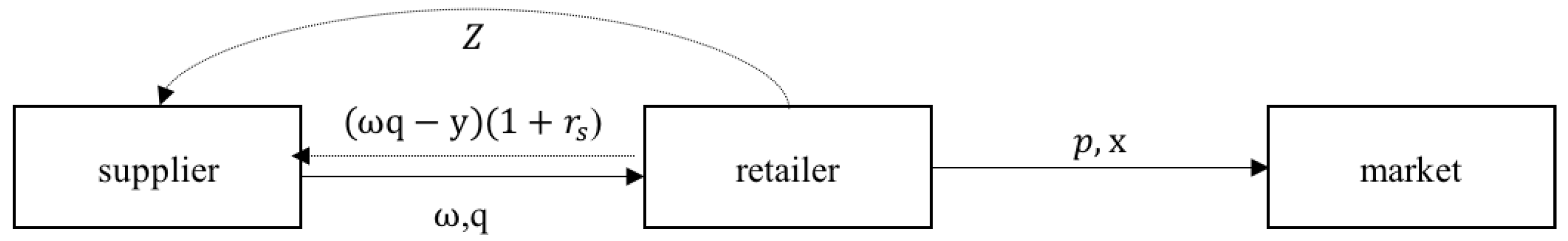
4.1. Internal Financing

Aiming at greater returns, the well-funded supplier is willing to provide financial support to the capital-strained retailer. This section mainly analyzes the retailer’s order decision and the supplier’s decision-making issue in the internal financing mode. The supplier is a leader. Although he cannot change the wholesale price, he is able to decide the loan interest according to different collateral assets of the retailer. The retailer is a follower, selecting the appropriate order quantity based on the market demand information, wholesale price and interest rate. In fact, the whole process is a two-stage Stackelberg sequential game with full information. Both sides pursue maximized expected returns. The sequence of events is the supplier firstly offers a take-it-or-leave-it internal financing contract ($\mathsf{\omega },{\mathrm{r}}_s$) to the retailer, if the retailer accepts the contract and uses internal financing, and then decides on an order quantity. To pursue the Stackelberg equilibrium results, we use the backward induction to solve the retailer’s optimal decision first.

(1) The retailer’s optimal strategy

Considering the retailer’s collateral assets, the supplier offers a suitable lending rate ${\mathrm{r}}_s$. Hence, the retailer’s optimization problem under the given financing mode can be formulated as ${\mathsf{\pi }}_1{}^{\mathrm{R}}$, Whether the loan obligation can be repaid or not depends on market conditions. Bankruptcy threshold ${\mathrm{B}}_1$ means then retailer can repay the whole loan $\left(\mathsf{\omega }\mathrm{q}-\mathrm{y}\right)\ast \left(1+{\mathrm{r}}_{\mathrm{s}}\right)$ when the market demand is greater than ${\mathrm{B}}_1$, otherwise the retailer falls through and the supplier bears the remaining loss.

According to the formula $\mathrm{px}+\mathrm{Z}=\left(\mathsf{\omega }\mathrm{q}-\mathrm{y}\right)\ast \left(1+{\mathrm{r}}_{\mathrm{s}}\right)$, we can get the retailer’s bankruptcy threshold ${\mathrm{B}}_1=\frac{\left(\mathsf{\omega }\mathrm{q}-\mathrm{y}\right)\left(1+{\mathrm{r}}_{\mathrm{s}}\right)-\mathrm{Z}}{\mathrm{p}}$.

The retailer’s expected profit is given by the formula (1):

$$\begin{array}{c}{{\mathsf{\pi }}_1}^{\mathrm{R}}={{\displaystyle \int }}_0^{{\mathrm{B}}_1}0f\left(\mathrm{x}\right)\mathrm{dx}+{{\displaystyle \int }}_{{\mathrm{B}}_1}^{\mathrm{q}}(\mathrm{p}\ast \mathrm{x}+\mathrm{Z}-\left(\mathsf{\omega }\mathrm{q}-\mathrm{y}\right)\ast \left(1+{\mathrm{r}}_{\mathrm{s}}\right))\ast f\left(\mathrm{x}\right)\mathrm{dx}\\ +{{\displaystyle \int }}_{\mathrm{q}}^{\infty }(\mathrm{p}\ast \mathrm{q}+\mathrm{Z}-\left(\mathsf{\omega }\mathrm{q}-\mathrm{y}\right)\ast \left(1+{\mathrm{r}}_{\mathrm{s}}\right))\ast f\left(\mathrm{x}\right)\mathrm{dx}-\mathrm{y}\end{array}$$

(1)

After some algebra, we can rewrite Equation (2) as:

$${{\mathsf{\pi }}_1}^{\mathrm{R}}=\mathrm{p}\ast \mathrm{q}+\mathrm{Z}-\mathrm{y}-\left(\mathsf{\omega }\mathrm{q}-\mathrm{y}\right)\ast \left(1+{\mathrm{r}}_{\mathrm{s}}\right)-{{\displaystyle \int }}_{{\mathrm{B}}_1}^{\mathrm{q}}\mathrm{p}\ast \mathrm{F}\left(\mathrm{x}\right)\mathrm{dx}$$

(2)

By analyzing the first-order derivatives of Equation (2) with respective to q, as the demand function conforms to IFR, $\frac{{\mathrm{d}\mathsf{\pi }}_1{}^{\mathrm{R}}}{\mathrm{dq}}=\mathrm{p}-\mathsf{\omega }\ast \left(1+{\mathrm{r}}_{\mathrm{s}}\right)-\mathrm{p}\ast \mathrm{F}\left(\mathrm{q}\right)+\mathrm{F}\left({\mathrm{B}}_1\right)\ast \mathsf{\omega }\ast \left(1+{\mathrm{r}}_{\mathrm{s}}\right);$ because of $\frac{{\mathrm{d}}^2{\mathsf{\pi }}_1{}^{\mathrm{R}}}{{\mathrm{dq}}^2}=-\mathrm{p}\ast f\left(\mathrm{q}\right)+f\left({\mathrm{B}}_1\right)\frac{{\left(\mathsf{\omega }\ast \left(1+{\mathrm{r}}_{\mathrm{s}}\right)\right)}^2}{\mathrm{p}}<0$, let $\frac{{\mathrm{d}\mathsf{\pi }}_1{}^{\mathrm{R}}}{\mathrm{dq}}=0$, We can get the expression(3) of the retailer’s profit-maximizing order quantity ${{\mathrm{q}}_1}^{\ast }$ under the lending rate, given by the supplier:

$${\mathrm{q}}_1{}^{\ast }={\mathrm{F}}^{-1}[1+{\Omega }_1\left(\mathrm{F}\left({\mathrm{B}}_1\right)-1\right],\mathrm{and}{\Omega }_1=\frac{\mathsf{\omega }\left(1+{\mathrm{r}}_{\mathrm{s}}\right)}{\mathrm{p}}$$

(3)

(2) The supplier’s optimal strategy

From our discussion in Section 4.1, the supplier offers the financing contract ($\mathsf{\omega },{\mathrm{r}}_s$) to the retailer at the beginning of sale season. Despite the salvage value of unsold items, the earnings depend on whether the retailer goes bankruptcy. Hence, the supplier’s expected profit is as Equation (4):

$${{\mathsf{\pi }}_1}^{\mathrm{s}}={{\displaystyle \int }}_0^{{\mathrm{B}}_1}\mathrm{p}\ast \mathrm{x}+\mathrm{Z}\ast f\left(\mathrm{x}\right)\mathrm{dx}+{{\displaystyle \int }}_{{\mathrm{B}}_1}^{\infty }\left(\mathsf{\omega }\mathrm{q}-\mathrm{y}\right)\left(1+{\mathrm{r}}_{\mathrm{s}}\right)\ast f\left(\mathrm{x}\right)\mathrm{dx}+\mathrm{y}-\mathrm{c}\ast \mathrm{q}$$

(4)

After some algebra, we can rewrite Equation (5) as

$${{\mathsf{\pi }}_1}^{\mathrm{s}}=\mathrm{y}+\left(\mathsf{\omega }\mathrm{q}-\mathrm{y}\right)\left(1+{\mathrm{r}}_{\mathrm{s}}\right)-{{\displaystyle \int }}_0^{{\mathrm{B}}_1}\mathrm{p}\ast \mathrm{F}\left(\mathrm{x}\right)\mathrm{dx}-\mathrm{c}\ast \mathrm{q}$$

(5)

By analyzing the first order derivatives of Formula (5) with respective to ${\mathrm{r}}_s$, there is an Equation (6)

$$\frac{{\mathrm{d}\mathsf{\pi }}_1{}^{\mathrm{s}}}{{\mathrm{dr}}_{\mathrm{s}}}=\left(\mathsf{\omega }\mathrm{q}-\mathrm{y}\right)\overline{\mathrm{F}}\left({\mathrm{B}}_1\right)+\left[\mathsf{\omega }\ast \left(1+{\mathrm{r}}_{\mathrm{s}}\right)\overline{\mathrm{F}}\left({\mathrm{B}}_1\right)-\mathrm{c}\right]\ast \frac{{\mathrm{dq}}_1{}^{\ast }}{\mathrm{dr}}$$

(6)

where $\frac{{\mathrm{dq}}_1{}^{\ast }}{\mathrm{dr}}=\frac{\left(\mathsf{\omega }\mathrm{q}-\mathrm{y}\right){\ast \Omega }_{1}f\left({\mathrm{B}}_1\right)-\mathsf{\omega }\overline{\mathrm{F}}\left({\mathrm{B}}_1\right)}{\mathrm{p}\left[f\left({\mathrm{q}}_1{}^{\ast }\right)-{\Omega }_1{}^{2}f\left({\mathrm{B}}_1\right)\right]}$. By substituting the equation $\frac{{\mathrm{dq}}_1{}^{\ast }}{\mathrm{dr}}$ into the equation $\frac{{\mathrm{d}\mathsf{\pi }}^{\mathrm{s}}}{\mathrm{dq}}$ and set $\frac{{\mathrm{d}\mathsf{\pi }}_1{}^{\mathrm{s}}}{{\mathrm{dr}}_{\mathrm{s}}}=0$, we have the expression (7) of the supplier’s optimal interest rate after simplification:

$${\mathrm{r}}^{\ast }=\frac{1}{\mathsf{\omega }\overline{\mathrm{F}}\left({\mathrm{B}}_1\right)}\ast \left[\mathrm{c}+\frac{\left(\mathrm{y}-\mathsf{\omega }\mathrm{q}\right)\overline{\mathrm{F}}\left({\mathrm{B}}_1\right)\ast \mathrm{p}\left(f\left({\mathrm{q}}_1{}^{\ast }\right)-{\Omega }_1{}^2\mathrm{f}\left({\mathrm{B}}_1\right)\right)}{\left(\mathsf{\omega }\mathrm{q}-\mathrm{y}\right){\ast \Omega }_{1}f\left({\mathrm{B}}_1\right)-\mathsf{\omega }\overline{\mathrm{F}}\left({\mathrm{B}}_1\right)}\right]$$

(7)

Lemma 1.

If the demand function is consistent with the IFR distribution, the capital-constrained retailer orders the less quantity of goods if the internal financing cost of the supplier is higher.

Proof. 

Referring to the process of verification of the relationship between the interest rate and order quantity by YAN et al. [41] and the definition of ${\mathsf{\pi }}_1{}^{\mathrm{R}}$ , the following Equation (8) can be obtained:

$$\frac{{\mathrm{dq}}_1{}^{\ast }}{{\mathrm{dr}}_{\mathrm{s}}}=\frac{\left({\mathsf{\omega }\mathrm{q}}^{\ast }-\mathrm{y}\right){\ast \Omega }_{1}f\left({\mathrm{B}}_1\right)-\mathsf{\omega }\ast \overline{\mathrm{F}}\left({\mathrm{B}}_1\right)}{\mathrm{p}\ast \left[f\left({\mathrm{q}}_1{}^{\ast }\right)-{\Omega }_1{}^{2}f\left({\mathrm{B}}_1\right)\right]}=\frac{\mathsf{\omega }\ast \left({\mathrm{q}}_1{}^{\ast }{\Omega }_{1}f\left({\mathrm{B}}_1\right)-\overline{\mathrm{F}}\left({\mathrm{B}}_1\right)\right)-{\mathrm{y}\ast \Omega }_{1}f\left({\mathrm{B}}_1\right)}{\mathrm{p}\ast \left[f\left({\mathrm{q}}_1{}^{\ast }\right)-{\Omega }_1{}^{2}f\left({\mathrm{B}}_1\right)\right]}$$

(8)

As $1<{\Omega }_1\le 1$, and the demand function is consistent with the IFR distribution, we have the following:

$${{\mathrm{q}}_1}^{\ast }{\Omega }_1\ast f\left({\mathrm{B}}_1\right)-\overline{\mathrm{F}}\left({\mathrm{B}}_1\right)=\mathrm{F}\left({\mathrm{B}}_1\right)\ast \left[1-\frac{{\mathrm{q}}_1{}^{\ast }{\Omega }_1\ast f\left({\mathrm{B}}_1\right)}{\overline{\mathrm{F}}\left({\mathrm{B}}_1\right)}\right]$$

where $\frac{{\mathrm{q}}_1{}^{\ast }{\Omega }_{1}f\left({\mathrm{B}}_1\right)}{\overline{\mathrm{F}}\left({\mathrm{B}}_1\right)}<\frac{{\mathrm{q}}_1{}^{\ast }\mathrm{f}\left({\mathrm{B}}_1\right)}{\overline{\mathrm{F}}\left({\mathrm{B}}_1\right)}<\frac{{\mathrm{q}}_1{}^{\ast }f\left({\mathrm{q}}_1{}^{\ast }\right)}{\overline{\mathrm{F}}\left({\mathrm{q}}_1{}^{\ast }\right)}\le 1$. It is clear to see that $-1+\frac{{\mathrm{q}}_1{}^{\ast }{\Omega }_{1}f\left({\mathrm{B}}_1\right)}{\overline{\mathrm{F}}\left({\mathrm{B}}_1\right)}<0$, which means ${{\mathrm{q}}_1}^{\ast }{\Omega }_{1}f\left({\mathrm{B}}_1\right)-\overline{\mathrm{F}}\left({\mathrm{B}}_1\right)<0$, besides $f\left({\mathrm{q}}_1{}^{\ast }\right)-{\Omega }_1{}^{2}f\left({\mathrm{B}}_1\right)>0$. Therefore, we can get $\frac{{\mathrm{dq}}_1{}^{\ast }}{{\mathrm{dr}}_{\mathrm{s}}}<0$. This completes the proof. □

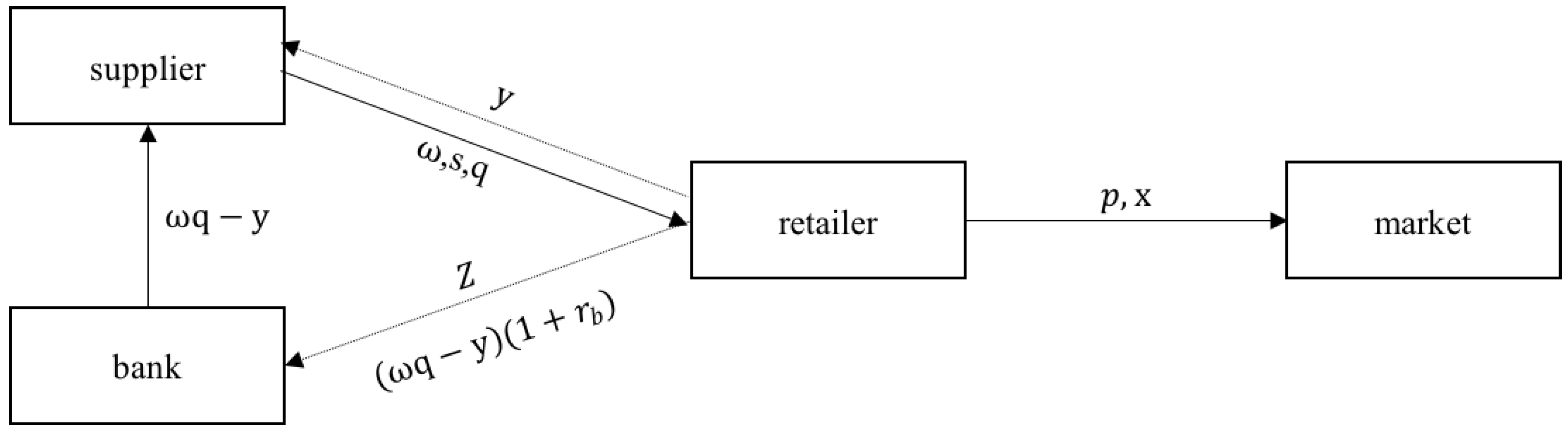
4.2. External Financing

Consider the situation that the retailer’s capital deficit can only be financed by bank loans under the supplier’s buy-back guarantee, which means the supplier will purchase the remaining goods of the retailer at the buy-back price $\mathrm{b}$. Therefore, the retailer can maximize the repayment of the bank’s principal and interest. In this financing mode, the supplier is still a well-funded leader, the retailer acts as a follower, and the bank is a sub-leader. All three parties seek to maximize their own profits. The sequence of moves is as same as follows. Firstly, the leader (supplier) decides the buy-back price $b$, which encourages the retailer to place more goods and achieve higher sales, and then, the sub-leader (bank) will accordingly evaluate the retailer’s financing conditions (collateral assets) and set a suitable lending rate to the retailer. After that, acting as the follower, the retailer decides how much to order according to the lending rate and the supplier’s wholesale price. To pursue the Stackelberg equilibrium results, we use the backward induction to solve the retailer’s optimal decision first.

(1) The retailer’s optimal strategy

Through external financing, the retailer’s procurement can run smoothly. Whether the loan obligation can be repaid completely or not also depends on the market condition. The term ${\mathrm{B}}_2$ represents the bankruptcy threshold of external financing; the retailer can repay the principal and interest of the bank loan $\left(\mathsf{\omega }\mathrm{q}-\mathrm{y}\right)\ast \left(1+{\mathrm{r}}_{\mathrm{b}}\right)$ when the market demand is greater than ${\mathrm{B}}_2$. If the product has a surplus, the supplier will buy back the rest of goods. Hence, the retailer’s optimization problem under the given financing mode can be formulated as ${\mathsf{\pi }}_2{}^{\mathrm{R}}$. According to $\mathrm{p}\ast \mathrm{x}+\mathrm{Z}=\left(\mathsf{\omega }\mathrm{q}-\mathrm{y}\right)\ast \left(1+{\mathrm{r}}_{\mathrm{b}}\right)$, we can get the retailer’s bankruptcy threshold: ${\mathrm{B}}_2=\frac{\left(\mathsf{\omega }\mathrm{q}-\mathrm{y}\right)\left(1+{\mathrm{r}}_{\mathrm{b}}\right)-\mathrm{b}\ast \mathrm{q}-\mathrm{Z}}{\mathrm{p}-\mathrm{b}}$.

The retailer’s expected profit is given by as formula (9):

$$\begin{array}{c}{{\mathsf{\pi }}_2}^{\mathrm{R}}={{\displaystyle \int }}_0^{{\mathrm{B}}_2}0f\left(\mathrm{x}\right)\mathrm{dx}+{{\displaystyle \int }}_{{\mathrm{B}}_2}^{\mathrm{q}}(\mathrm{p}\ast \mathrm{x}+\mathrm{Z}+\mathrm{b}\ast \left(\mathrm{q}-\mathrm{x}\right)-\left(\mathsf{\omega }\mathrm{q}-\mathrm{y}\right)\left(1+{\mathrm{r}}_{\mathrm{b}}\right))\ast f\left(\mathrm{x}\right)\mathrm{dx}\\ +{{\displaystyle \int }}_{\mathrm{q}}^{\infty }(\mathrm{p}\ast \mathrm{q}+\mathrm{Z}-\left(\mathsf{\omega }\mathrm{q}-\mathrm{y}\right)\left(1+{\mathrm{r}}_{\mathrm{b}}\right))\ast f\left(\mathrm{x}\right)\mathrm{dx}-\mathrm{y}\end{array}$$

(9)

After simplification, we can rewrite Equation (10) as

$${{\mathsf{\pi }}_2}^{\mathrm{R}}=\mathrm{p}\ast \mathrm{q}+\mathrm{Z}-\left(\mathsf{\omega }\mathrm{q}-\mathrm{y}\right)\left(1+{\mathrm{r}}_{\mathrm{b}}\right)-\mathrm{y}-{{\displaystyle \int }}_{{\mathrm{B}}_2}^{\mathrm{q}}\left(\mathrm{p}-\mathrm{b}\right)\ast \mathrm{F}\left(\mathrm{x}\right)\mathrm{dx}$$

(10)

By analyzing the first-order derivatives of Equation (10) with respective to q, there is the Equation (11) as follows:

$$\frac{{\mathrm{d}\mathsf{\pi }}_2{}^{\mathrm{R}}}{\mathrm{dq}}=\mathrm{p}-\mathsf{\omega }\ast \left(1+{\mathrm{r}}_{\mathrm{b}}\right)-\left(\mathrm{p}-\mathrm{b}\right)\ast \mathrm{F}\left(\mathrm{q}\right)+\mathrm{F}\left({\mathrm{B}}_2\right)\ast \left(\mathsf{\omega }\ast \left(1+{\mathrm{r}}_{\mathrm{b}}\right)-\mathrm{b}\right)$$

(11)

Due to the second derivative $\frac{{\mathrm{d}}^2{\mathsf{\pi }}_2{}^{\mathrm{R}}}{{\mathrm{dq}}^2}=-\left(\mathrm{p}-\mathrm{b}\right)\ast f\left(\mathrm{q}\right)+f\left({\mathrm{B}}_2\right)\ast \frac{{\left(\mathsf{\omega }\left(1+{\mathrm{r}}_{\mathrm{b}}\right)-\mathrm{b}\right)}^2}{\mathrm{p}-\mathrm{b}}<0$, set $\frac{{\mathrm{d}\mathsf{\pi }}_2{}^{\mathrm{R}}}{\mathrm{dq}}=0$. Given the lending rate by the bank, we can figure out the retailer’s optimal order quantity ${\mathrm{q}}_2{}^{\ast }$ as expression (12):

$${\mathrm{q}}_2{}^{\ast }={\mathrm{F}}^{-1}\left[{\Omega }_2\ast \mathrm{F}\left({\mathrm{B}}_2\right)+\frac{\mathrm{p}-\mathsf{\omega }\left(1+{\mathrm{r}}_{\mathrm{b}}\right)}{\mathrm{p}-\mathrm{b}}\right],\mathrm{and}{\Omega }_2=\frac{\mathsf{\omega }\left(1+{\mathrm{r}}_{\mathrm{b}}\right)-\mathrm{b}}{\mathrm{p}-\mathrm{b}}$$

(12)

(2) The bank’s optimal strategy

At the end-of-season sale, whether the bank’s loan can be covered entirely not depends on the market condition, the value of collateral assets, and the salvage value of unsold goods.

If the retailer does not go bankrupt, the bank can get the principal and interest of the loan $\left(\mathsf{\omega }\mathrm{q}-\mathrm{y}\right)\ast \left(1+{\mathrm{r}}_{\mathrm{b}}\right)$, otherwise the bank can only receive $\mathrm{p}\ast \mathrm{x}+\mathrm{Z}+\mathrm{b}\ast \left(\mathrm{q}-\mathrm{x}\right)$. In view of the above, the bank’s expected profit is as formula (13):

$$\begin{array}{c}{\mathsf{\pi }}^{\mathrm{b}}={{\displaystyle \int }}_0^{{\mathrm{B}}_2}\mathrm{p}\ast \mathrm{x}+\mathrm{Z}f\left(\mathrm{x}\right)\mathrm{dx}+{{\displaystyle \int }}_{{\mathrm{B}}_2}^{\infty }\left(\mathsf{\omega }\mathrm{q}-\mathrm{y}\right)\left(1+{\mathrm{r}}_{\mathrm{b}}\right)f\left(\mathrm{x}\right)\mathrm{dx}-\left(\mathrm{wq}-\mathrm{y}\right)\\ =\left(\mathsf{\omega }\mathrm{q}-\mathrm{y}\right)(1+{\mathrm{r}}_{\mathrm{b}})-{{\displaystyle \int }}_0^{{\mathrm{B}}_2}\left(\mathrm{p}-\mathrm{b}\right)\ast \mathrm{F}\left(\mathrm{x}\right)\mathrm{dx}\end{array}$$

(13)

By analyzing the first-order derivatives of Equation (14) with respective to ${\mathrm{r}}_b$, we can figure out the Equation (14):

$$\frac{{\mathrm{d}\mathsf{\pi }}^{\mathrm{b}}}{{\mathrm{dr}}_{\mathrm{b}}}=\left(\mathsf{\omega }\mathrm{q}-\mathrm{y}\right)-\left(\mathsf{\omega }\mathrm{q}-\mathrm{y}\right)\ast \mathrm{F}\left({\mathrm{B}}_2\right)+\left[\mathsf{\omega }\ast \left(1+{\mathrm{r}}_{\mathrm{b}}\right)+{\Omega }_2\mathrm{F}\left({\mathrm{B}}_2\right)\right]\ast \frac{{\mathrm{dq}}_2{}^{\ast }}{\mathrm{dr}}$$

(14)

Due to $\frac{{\mathrm{dq}}_2{}^{\ast }}{{\mathrm{dr}}_{\mathrm{b}}}=\frac{\left({\mathsf{\omega }\mathrm{q}}_2{}^{\ast }-\mathrm{y}\right){\ast \Omega }_2\mathrm{f}\left({\mathrm{B}}_2\right)-\mathsf{\omega }\ast \overline{\mathrm{F}}\left({\mathrm{B}}_2\right)}{\left(\mathrm{p}-\mathrm{b}\right)\ast \left[\mathrm{f}\left({\mathrm{q}}_2{}^{\ast }\right)-{\Omega }_2{}^2\mathrm{f}\left({\mathrm{B}}_2\right)\right]}$, by substituting Equation $\frac{{\mathrm{dq}}_2{}^{\ast }}{{\mathrm{dr}}_{\mathrm{b}}}$ into Equation $\frac{{\mathrm{d}\mathsf{\pi }}^{\mathrm{b}}}{{\mathrm{dr}}_{\mathrm{b}}}$, set $\frac{{\mathrm{d}\mathsf{\pi }}^{\mathrm{b}}}{{\mathrm{dr}}_{\mathrm{b}}}=0$. We have the expression (15) of the optimal lending rate under the optimal ordering quantity given by the retailer:

$${{\mathrm{r}}_{\mathrm{b}}}^{\ast }=\left[\frac{\left(\mathrm{y}-{\mathsf{\omega }\mathrm{q}}_2{}^{\ast }\right)\overline{\mathrm{F}}\left({\mathrm{B}}_2\right)\times \left(\mathrm{p}-\mathrm{b}\right)\left(f\left({\mathrm{q}}_2{}^{\ast }\right)-{\Omega }_2{}^2\mathrm{f}\left({\mathrm{B}}_2\right)\right)}{\mathsf{\omega }\left({\mathsf{\omega }\mathrm{q}}_2{}^{\ast }-\mathrm{y}\right)\times {\Omega }_{2}f\left({\mathrm{B}}_2\right)-\mathsf{\omega }\overline{\mathrm{F}}\left({\mathrm{B}}_2\right)}\right]+\frac{\left(\mathsf{\omega }\left(1+{\mathrm{r}}_{\mathrm{b}}\right)-\mathrm{b}\right)\mathrm{F}\left({\mathrm{B}}_2\right)}{\mathsf{\omega }}-1$$

(15)

Lemma 2.

If the demand function is consistent with the IFR distribution, the capital-constrained retailer orders the less quantity of goods if the external financing cost with the supplier is higher.

The proof is the same as that for the process of Lemma 1.

(3) The Supplier’s optimal strategy

Finally, we consider the optimization question faced with the supplier. If the order quantity is less than the market demand, the supplier does not have to buy goods back, otherwise the supplier provides the buy-back contract. By this way, the supplier bears the partial risk of market fluctuation. At the same time, this way can encourage the retailer to place further goods and promise that the buy-back amount is not excessive, so the expected profit of the supplier is:

$${{\mathsf{\pi }}_2}^{\mathrm{s}}=\left(\mathsf{\omega }-\mathrm{c}\right)\mathrm{q}-\mathrm{b}{{\displaystyle \int }}_0^{\mathrm{q}}\left(\mathrm{q}-\mathrm{x}\right)f\left(\mathrm{x}\right)\mathrm{dx}=\left(\mathsf{\omega }-\mathrm{c}\right)\mathrm{q}-\mathrm{b}{{\displaystyle \int }}_0^{\mathrm{q}}\mathrm{F}\left(\mathrm{x}\right)\mathrm{dx}$$

(16)

By analyzing the first-order derivatives of Equation (16) with respective to $\mathrm{b}$, the derivative of ${\mathsf{\pi }}_2{}^{\mathrm{s}}$ is given by as the Equation (17):

$$\frac{{\mathrm{d}\mathsf{\pi }}_2{}^{\mathrm{s}}}{\mathrm{db}}=\left[\mathsf{\omega }-\mathrm{c}-\mathrm{b}\ast \mathrm{F}\left(\mathrm{q}\right)\right]\ast \frac{\mathrm{dq}}{\mathrm{db}}-{{\displaystyle \int }}_0^{\mathrm{q}}\mathrm{F}\left(\mathrm{x}\right)\mathrm{dx}$$

(17)

Due to $\frac{{\mathrm{dq}}_2{}^{\ast }}{\mathrm{db}}=\frac{\left(\mathrm{p}-\mathsf{\omega }\left(1+{\mathrm{r}}_{\mathrm{b}}\right)\right)\ast \overline{\mathrm{F}}\left({\mathrm{B}}_2\right)+\left({\mathsf{\omega }\ast \mathrm{q}}_2{}^{\ast }-\mathrm{y}\right)\left(1+{\mathrm{r}}_{\mathrm{b}}\right)-{\mathrm{p}\ast \mathrm{q}}_2{}^{\ast }-\mathrm{Z}}{{\left(\mathrm{p}-\mathrm{b}\right)}^2\ast \left[\mathrm{f}\left({\mathrm{q}}_2{}^{\ast }\right)-{\Omega }_1{}^2\mathrm{f}\left({\mathrm{B}}_2\right)\right]}$, by substituting Equation $\frac{{\mathrm{dq}}_2{}^{\ast }}{\mathrm{db}}$ into Equation $\frac{{\mathrm{d}\mathsf{\pi }}_2{}^{\mathrm{s}}}{\mathrm{db}}$, set $\frac{{\mathrm{d}\mathsf{\pi }}_2{}^{\mathrm{s}}}{\mathrm{db}}=0$. Hence, $\left[\mathsf{\omega }-\mathrm{c}-\mathrm{b}\ast \mathrm{F}\left(\mathrm{q}\right)\right]\ast \frac{\left(\mathrm{p}-\mathsf{\omega }\left(1+{\mathrm{r}}_{\mathrm{b}}\right)\right)\overline{\mathrm{F}}\left({\mathrm{B}}_2\right)+\left(\left({\mathsf{\omega }\mathrm{q}}_2{}^{\ast }-\mathrm{y}\right)\left(1+{\mathrm{r}}_{\mathrm{b}}\right)-{\mathrm{p}\ast \mathrm{q}}_2{}^{\ast }-\mathrm{Z}\right){\ast \Omega }_{1}f\left({\mathrm{B}}_2\right)}{{\left(\mathrm{p}-\mathrm{b}\right)}^2\ast \left[f\left({\mathrm{q}}_2{}^{\ast }\right)-{\Omega }_1{}^{2}f\left({\mathrm{B}}_2\right)\right]}-{{\displaystyle \int }}_0^{\mathrm{q}}\mathrm{F}\left(\mathrm{x}\right)\mathrm{dx}=0$. We can see the optimal buy-back price by calculation.

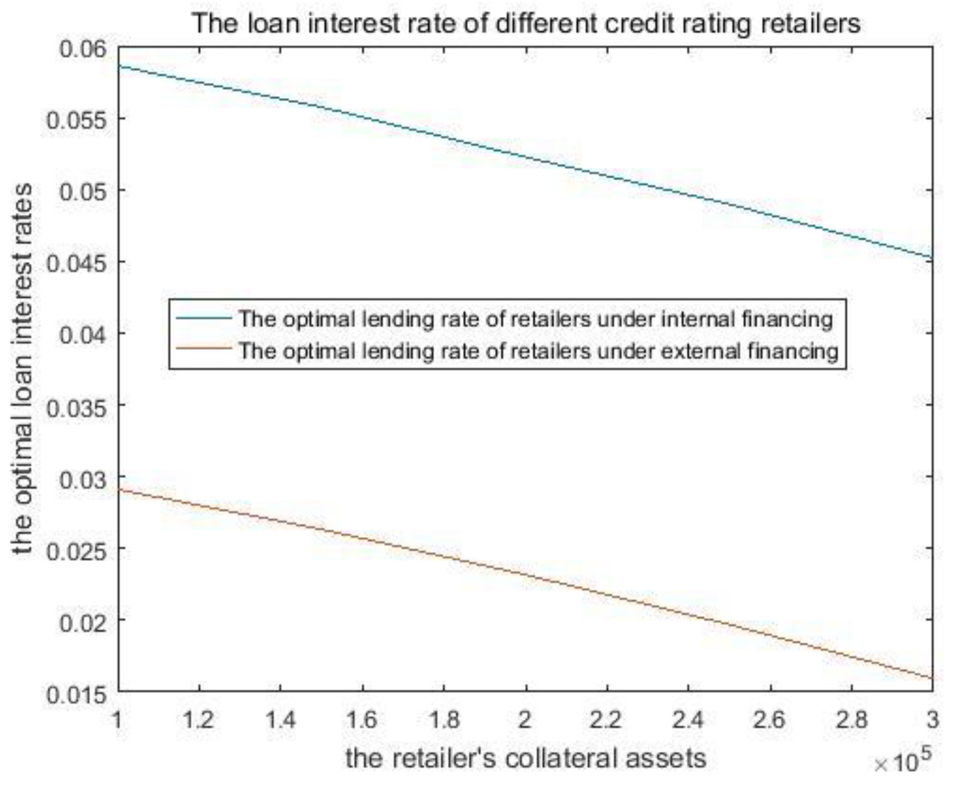
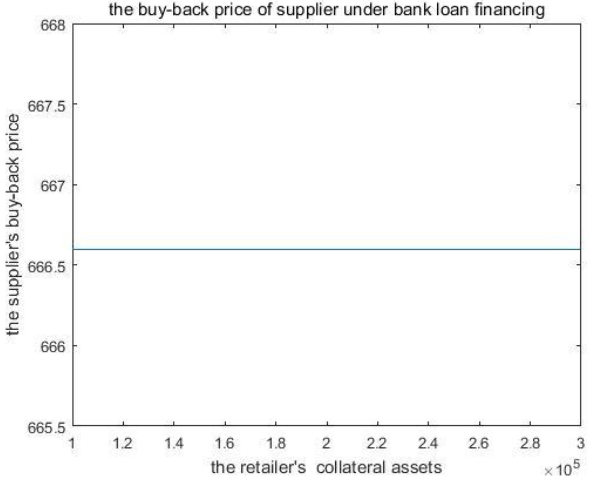
5. Numerical Examples

This section firstly examines changes of the supplier’s buy-back price and the optimal lending rates of the bank and the supplier, owing to retailer’s different collateral assets under different financing modes; then, we calculated each participant’s expected profit under the different collateral assets of the retailer. We also compared the differences between the two financing modes.

In order to ensure the authenticity and practicality of test results, we referred to the parameter design method of numerical simulation in related literature [39,41], and investigated the operation data of the enterprise related to this research topic, and finally determined the reliable data parameters. We assumed that the market demand obeys the uniform distribution on [500, 1000], and fix $\mathrm{p}=1000,\mathrm{w}=700,\mathrm{y}=100,000,\mathrm{c}=300$. Under the classic newsboy model, satisfying $\mathsf{\omega }\ast \mathrm{q}>\mathrm{y}$ and $\mathrm{p}>\mathsf{\omega }\left(1+\mathrm{r}\right)$, we set that the retailer’s collateral assets fluctuate from 100,000 to 300,000. It is easy to determine the supplier’s optimal lending rate in the internal financing mode, and the optimal buy-back price of the supplier and the bank’s optimal lending rate in the external financing mode, respectively.

Comparing with the different lending rates in Figure 3, we can clearly find the optimal loan interest rate for external financing is relatively lower, which means the external financing with a buy-back guarantee is superior to the internal financing. It reveals the buy-back contract enables the bank to hold an optimistic attitude for the retailer’s debt-paying ability. When both financing modes exist, the retailer should give the priority to the external financing. Moreover, it can be clearly seen that the optimal lending rate decreases with the increasing of retailer’s collateral assets, which uncovers the more collateral assets a retailer has and the lower the lending rate. According to the Lemmas 1 and 2, this explanation reflects from one respect: the retailer will place further goods as the lending rate has fallen.

From Figure 4, some results were obtained, which are different from the intuitive judgment. With all other variables remaining unchanged, the retailer’s collateral assets will not affect the optimal buy-back price of the supplier, which may be due to the fact that the supplier has offered the relatively reasonable buy-back price to repurchase the remaining goods of the retailer. Consequently, he is not likely to raise the buy-back price because this move will lead to lower profits.

According to

Table 2. The optimal order quantities and expected profits of two financing modes.

Collateral Asset	Internal Financing			External Financing
$\mathbf{Z}$	${\mathbf{q}}_1{}^{\ast }$	${\mathsf{\pi }}_1{}^{\mathbf{R}}$	${\mathsf{\pi }}_1{}^{\mathbf{s}}$	${\mathbf{q}}_2{}^{\ast }$	${\mathsf{\pi }}_2{}^{\mathbf{R}}$	${\mathsf{\pi }}_2{}^{\mathbf{s}}$	${\mathsf{\pi }}^{\mathbf{b}}$
100,000	612	251,352	254,504	653	284,195	262,904	363,494
120,000	633	271,625	263,099	676	307,312	275,888	384,396
140,000	657	291,576	272,594	703	330,295	281,804	403,836
160,000	682	309,586	283,557	734	352,822	290,978	426,214
180,000	704	327,980	291,240	765	374,387	301,112	448,565
200,000	739	341,627	306,465	799	394,999	314,300	468,486
220,000	762	358,286	314,303	832	414,488	327,192	489,724
240,000	784	372,104	323,796	858	433,318	337,282	508,111
260,000	816	382,326	337,607	890	450,950	342,050	521,250
280,000	844	392,778	349,686	922	467,558	357,842	534,893
300,000	872	400,248	351,786	953	483,295	363,804	545,758

, it is obvious to see that the optimal order quantity goes up continuously when the retailer’s collateral assets increase, which illustrates that he is confident in repaying the loan and prefers to believe the bright market demand because of the lower lending rates. At the same time, compared with the internal financing mode, we find that each participant can obtain the higher expected profit under the external financing mode. This also explains why the supplier is willing to provide the buy-back contact with the retailer, which not only encourages the retailer to order more goods but also gives him an opportunity to loan from the bank. Besides, with the increase in the retailer’s collateral assets, the profit of each party will be expected to climb slightly. This is because the supplier and the bank tend to hold optimistic attitudes for the retailer’s repaying ability.

6. Conclusions

In this paper, we formulated two different financing modes, which are widely used in SCF practices but have never been researched in existing literature. As a matter of fact, the most outstanding contribution of this study lies in the fact that we had an initial attempt to examine how the retailer’s collateral assets, measuring the trade grade, affect the lending rates of different financing modes, which are more accordance with practical circumstances of enterprises. Furthermore, in the past research, the scholars tend to ignore the bankruptcy risk in order to simplify the model. Here, we not only considered the bankruptcy risk but also matched it with the enterprise’s real operational condition, which attributes to an increase of practical value of our model. In particular, we focused on comparative analysis of optimal decisions between these two different modes using the numerical examples, because it is hard to derive a visual comparison. Through our analysis, we established the following major results.

Firstly, the study finds that regardless of which financing mode is chosen, the capital-constrained retailer orders fewer goods if the financing cost is higher. Secondly, when the market demand obeys the uniform distribution, if the retailer possesses more collateral assets, he will enjoy a lower lending rate and order more goods. Apart from that, the external financing can provide a lower lending rate than the internal financing, because the well-funded supplier offers a buy-back guarantee to the retailer. Surprisingly, we also see that the scale of the collateral assets will not affect the buy-back price provided by the supplier. Finally, it is easy to observe that each participant can obtain the higher expected profits in the external profits.

Hence, the supplier could cooperate with the bank and then the retailer to achieve the Stackelberg equilibrium results. In particular, the capital-constrained supplier makes full use of the buy-back contract to enable the distressed retailer to finance from the bank, instead of offering internal financing. We hope our results could offer an effective method and scientific basis for each participant to make decisions on project financing.

Certainly, as a complex SCF system, we assume that the decision makers are risk-neutral. With the implementation of the New Basel Capital Accord, the future research should take the risk control of each participant into account. In addition, this study merely considers the retailer’s bankruptcy risk neglecting the bankruptcy risk of the supplier, which seems to have some limitations because comprehensive consideration will be more conducive for the decision maker.

References

1. Li, Y.; Chen, T.; Xin, B. Optimal Financing Decisions of Two Cash-Constrained Supply Chains with Complementary Products. Sustainability 2016, 8, 429. [Google Scholar] [CrossRef]
2. Wang, Y.; Shao, Y.H.; Ou, J.Q. The Research on Trade Credit Short-term Financing in a Capital-constrained Supply Chain. In Proceedings of the International Conference on Management Science and Management Innovation, Changsha, China, 14–15 June 2014. [Google Scholar]
3. Archibald, T.W.; Thomas, L.C.; Betts, J.M.; Johnston, R.B. Should start up companies be cautious? Inventory policies which maximise survival probabilities. Manag. Sci. 2002, 48, 1161–1174. [Google Scholar] [CrossRef]
4. Liu, X.; Zhou, L.; Wu, Y.C.J. Supply Chain Finance in China: Business Innovation and Theory Development. Sustainability 2015, 7, 14689–14709. [Google Scholar] [CrossRef] [Green Version]
5. Boschi, M.; Girardi, A.; Ventura, M. Partial credit guarantees and SMEs financing. J. Financ. Stab. 2014, 15, 182–194. [Google Scholar] [CrossRef]
6. Serrasqueiro, Z.; Nunes, P.M. Financing behaviour of Portuguese SMEs in hotel industry. Int. J. Hosp. Manag. 2014, 43, 98–107. [Google Scholar] [CrossRef]
7. Wolter, M.; Rösch, D. Cure events in default prediction. Eur. J. Oper. Res. 2014, 238, 846–857. [Google Scholar] [CrossRef]
8. Ono, A.; Uesugi, I. Role of Collateral and Personal Guarantees in Relationship Lending: Evidence from Japan’s SME Loan Market. J. Money Credit. Bank. 2010, 41, 935–960. [Google Scholar] [CrossRef]
9. Buzacott, J.A.; Zhang, R.Q. Inventory Management with Asset-Based Financing. Manag. Sci. 2004, 50, 1274–1292. [Google Scholar] [CrossRef]
10. Niinimäki, J.-P. Nominal and true cost of loan collateral. J. Bank. Financ. 2011, 35, 2782–2790. [Google Scholar] [CrossRef]
11. Rubin, J.; Wagner, R. Destroying collateral: Asset security and the financing of firms. Appl. Econ. Lett. 2015, 22, 704–709. [Google Scholar] [CrossRef]
12. Voordeckers, W.; Steijvers, T. Business collateral and personal commitments in SME lending. J. Bank. Financ. 2006, 30, 3067–3086. [Google Scholar] [CrossRef] [Green Version]
13. Trott, P. How SMEs can benefit from supply chain partnerships. Int. J. Prod. Res. 2015, 53, 1527–1543. [Google Scholar]
14. Yang, S.A.; Birge, J.R.; Parker, R.P. The Supply Chain Effects of Bankruptcy. Manag. Sci. 2015, 61, 2320–2338. [Google Scholar] [CrossRef]
15. Das, P.K. Financing Pattern and Utilization of Fixed Assets—A Study. Asian J. Soc. Sci. Stud. 2017, 2, 20–28. [Google Scholar] [CrossRef]
16. Petersen, M.A.; Rajan, R.G. Trade Credit: Theory and Evidence. Rev. Financ. Stud. 1997, 10, 661–691. [Google Scholar] [CrossRef]
17. Arnold, J.; Minner, S. Financial and operational instruments for commodity procurement in quantity competition. Int. J. Prod. Econ. 2011, 131, 96–106. [Google Scholar] [CrossRef]
18. Kouvelis, P.; Zhao, W. The Newsvendor Problem and Price-Only Contract When Bankruptcy Costs Exist. Produ. Oper. Manag. 2011, 20, 921–936. [Google Scholar] [CrossRef]
19. Lee, C.H.; Rhee, B.D. Coordination contracts in the presence of positive inventory financing costs. Int. J. Prod. Econ. 2010, 124, 331–339. [Google Scholar]
20. Lee, C.H.; Rhee, B.D. Trade credit for supply chain coordination. Eur. J. Oper. Res. 2011, 214, 136–146. [Google Scholar] [CrossRef]
21. Yan, N.; Sun, B. Comparative analysis of supply chain financing strategies between different financing modes. J. Ind. Manag. Optim. 2015, 11, 1073–1087. [Google Scholar] [CrossRef]
22. Fisman, R.; Raturi, M. Does Competition Encourage Credit Provision? Evidence from African Trade Credit Relationships. Rev. Econ. Stat. 2004, 86, 345–352. [Google Scholar] [CrossRef]
23. Yang, S.A.; Birge, J.R. How Inventory Is (Should Be) Financed: Trade Credit in Supply Chains with Demand Uncertainty and Costs of Financial Distress; Working Paper; The University of Chicago Booth School of Business: Chicago, IL, USA, 2011. [Google Scholar]
24. Federgruen, A.; Wang, M. Inventory Subsidy versus Supplier Trade Credit in Decentralized Supply Chains; Working Paper; Columbia Business School: New York, NY, USA, 2010. [Google Scholar]
25. Cressy, R.; Olofsson, C. The Financial Conditions for Swedish SMEs: Survey and Research Agenda. Small Bus. Econ. 1997, 9, 179–194. [Google Scholar] [CrossRef]
26. Meyer, L.H. The present and future roles of banks in small business finance. J. Bank. Financ. 1998, 22, 1109–1116. [Google Scholar] [CrossRef]
27. Bernanke, B.S.; Blinder, A.S. The Federal Funds Rate and the Channels of Monetary Transmission. Am. Econ. Rev. 1992, 82, 901–921. [Google Scholar]
28. Chen, X.F.; Zhu, D.L.; Ying, W.J. Financial and operation decisions in budget-constrained supply chain. J. Manag. Sci. China 2008, 11, 70–77. [Google Scholar]
29. Caldentey, R.; Chen, X. The role of financial services in procurement contracts. In The Handbook of Integrated Risk Management in Global Supply Chains; John Wiley & Sons: Hoboken, NJ, USA, 2011. [Google Scholar]
30. Wilner, B.S. The Exploitation of Relationships in Financial Distress: The Case of Trade Credit. J. Financ. 2000, 55, 153–178. [Google Scholar] [CrossRef] [Green Version]
31. Baird, D.G.; Picker, R.C. A Simple Non-Cooperative Bargaining Model of Corporate Reorganizations. J. Legal Stud. 1991, 20, 311–349. [Google Scholar] [CrossRef]
32. Bebchuk, L.A.; Chang, H.F. Bargaining and the Division of Value in Corporate Reorganization. J. Law Econ. Organ. 1992, 8, 253–279. [Google Scholar]
33. Kordana, K.A.; Posner, E.A. A Positive Theory of Chapter 11. Soc. Sci. Electron. Publ. 1999, 74, 161–234. [Google Scholar] [CrossRef]
34. Kouvelis, P.; Zhao, W. Financing the Newsvendor: Supplier vs. Bank, and the Structure of Optimal Trade Credit Contracts. Oper. Res. 2012, 60, 566–580. [Google Scholar] [CrossRef]
35. Padmanabhan, V.; Png, I.P.L. Returns Policies: Make Money by Making Good. Sloan Manag. Rev. 1995, 37, 65–72. [Google Scholar]
36. Pasternack, B.A. Optimal pricing and return policies for perishable commodities. Mark. Sci. 2008, 27, 133–140. [Google Scholar] [CrossRef]
37. Liu, J.; Wu, C. Study of a tow-level supply chain returns policy model based on the newsboy model. Chin. J. Manag. Sci. 2010, 18, 73–78. [Google Scholar]
38. Wu, D. Coordination of competing supply chains with news-vendor and buyback contract. Int. J. Prod. Econ. 2013, 144, 1–13. [Google Scholar] [CrossRef]
39. Wang, Z.; Ma, Z.; Zhou, Y. Financing Decisions for Confirming Warehouse with core enterprise’s Buyback Guarantee. Chin. J. Manag. Sci. 2016, 24, 162–169. [Google Scholar]
40. Zhong, Y.; Zhou, Y.; Li, B.; Wang, S. The retailer’s optimal ordering and pricing policies with supply chain financing. J. Manag. Sci. China 2011, 14, 57–67. [Google Scholar]
41. Yan, N.; Sun, B. Optimal strategies for supply chain financing system based on warehouse receipts financing with credit line. Syst. Eng.-Theory Pract. 2011, 31, 1674–1679. [Google Scholar]
Figure 1. Framework of internal financing.
Sustainability 10 03045 g001
Figure 2. Framework of external financing.
Sustainability 10 03045 g002
Figure 3. The optimal lending rates of different collateral assets.
Sustainability 10 03045 g003
Figure 4. The optimal buy-back prices of different collateral asset.
Sustainability 10 03045 g004