Integration of Demand Response and Photovoltaic Resources in Residential Segments

Abstract

The development of renewable sources in residential segments is basic to achieve a sustainable energy scenario in the horizon 2030–2050 because these segments explain around 25% of the final energy consumption. Demand Response and its effective coordination with renewable are additional concerns for residential segments. This paper deals with two problems: the demonstration of cost-effectiveness of renewables in three different scenarios, and the application of the flexibility of demand, performing as energy storage systems, to efficiently manage the generation of renewable sources while improving benefits and avoiding penalties for the customer. A residential customer in Spain has been used as example. The work combines the use of a commercial simulator to obtain photovoltaic generation, the monitoring of customer to obtain demand patterns, and the development of a Physically-Based Model to evaluate the capability of demand to follow self-generation. As a main result, the integration of models (load/generation), neglected in practice in other approaches in the literature, allows customers to improve revenue up to 20% and reach a basic but important knowledge on how they can modify the demand, development of new skills and, in this way, learn how to deal with the characteristics and limitations of both Demand and Generation when a customer becomes a prosumer. This synergy amongst demand and generation physically-based models boosts the possibilities of customers in electricity markets.

1. Introduction

1.1. Current Status of Renewable Sources in Europe

In 2016, the European Union (EU) primary energy imports from non-member countries reached 53.61% of all primary energy consumption [1]. This fact clearly exposes that energy security from EU depends heavily on external countries. In order to reduce the dependency on energy imports, particularly of oil and gas, and guarantee the energy supply, it is necessary to increase the share of renewable energy sources (RES).

Because of this, in recent years, the development of RES has been a priority in European policies. In 2009, Directive 2009/28/EC has been published to promote the use of energy from RES, reduce greenhouse gas (GHG) emissions, and increase energy efficiency [2]. The main objectives of this regulation are a 20% reduction of GHG emission (related to 1990 levels), a 20% improvement in energy efficiency, and a renewable generation share of 20% in 2020. To achieve these targets, each member of the EU had to adopt a National Renewable Energy Plan adapted to the peculiarities and abilities of the states to increase RES in the generation mix.

As a result of this regulation, the renewable energy share of the European Union increased every year and reached 17.7% in 2017, as it is shown in Figure 1.

Current predictions confirm that it will be possible to meet the 2020 targets. Several improvements in energy use intensity have been achieved in the last years due to an increase in the efficiency of buildings, industries, manufacturing processes, products, and transport.

The highest RES growth has occurred in the electricity sector, which has experienced an increase from 15.35% in 2006 to 29.6% in 2016 [3]. Figure 2 shows the evolution of electricity generation from the main renewable sources between 2000 and 2016 in EU-28 (in TWh).

In 2015, hydropower was still the main renewable electricity source with 38% of total renewable generation [4]. However, due to the high cost of building new hydropower plants and their potential environmental impact, the amount of energy generation has remained approximately the same since 1990, standing at around 300 TWh [5].

Regarding wind power, wind generation plants have experienced a strong deployment, increasing the installed capacity four times from 2004 to 2015, reaching 33% of the generation mix. Germany and Spain are the countries that have contributed the most in onshore wind generators, while Sweden, the United Kingdom, Denmark, and Germany have installed a large amount of offshore wind generation capacity. This technology, especially offshore plants, still has an important margin of development that can be increased in the near future.

Finally, it is important to highlight the contribution of solar photovoltaic (PV) energy, accounting for a 12% share of all renewable generation in 2015. The PV development has experienced a growth peak between 2011 and 2012, but the growth rates have decreased since then. The rapid growth of solar plants is driven by a fast technological progress and an important cost reduction.

Also, PV energy has allowed directly involving final consumers in energy transition and making them participant in environmental policies. The option of installing a few PV modules in dwellings has encouraged the deployment of this type of generation, which allows consumers to produce their own electricity (known as “prosumers”) and save on their energy bill. Germany, Spain and Italy are the countries with the leading amount of kW installed in Europe, producing 38% of Solar PV energy in Europe [4].

Spain has the highest solar global irradiation levels of Europe, with a yearly average around 1600 kWh/m², which exceeds 2200 kWh/m² in some locations (levels are only comparable with Italy, Greece, Malta, and Portugal in the EU-27 [6]). For these reasons, the south of Spain has been chosen for this study.

Photovoltaics in Spain

In Spain, solar PV has had uneven development. Between 2007 and 2008, due to an auspicious regulation, the growth of solar PV installations was much faster than expected. In 2008, Spain was one of the countries who installed more solar PV power (2733 MW), reaching a total capacity of 3351 MW [4]. Nevertheless, subsequent changes in regulation broke this deployment. In 2017, total installed capacity was 4978 MW. This means that for eight years, total solar capacity installed only increased by 1637 MW (Figure 3).

For the first time, in 2017, Spain disappeared from the top ten countries with the highest installed capacity [4]. In 2017, solar PV generation accounted for 3.2% of all electricity generation in Spain.

1.2. European Commission Environmental Policies and Objectives: Energy Framework 2030–2050

After the success of the measures and policies implemented by Directive 2009/28/EC [2], it was expected the development of a new framework aimed at the improvement of energy efficiency and the reduction of environmental impacts inside the EU-28.

According to these objectives, in 2011 the European Commission published the documents “A roadmap for moving to a competitive low carbon economy in 2050” [7] and “Energy Roadmap 2050” [8]. These documents show that by 2050, GHG emissions should be reduced by 80% from 1990 levels. To achieve these goals, in 2030 emissions must be cut by 40% and by 60% in 2040. In addition, it is necessary to engage all energy sectors: electricity, transportation, buildings, industries, and agriculture. The reports also point out that the stated objectives are feasible and affordable but require innovation and strong investments.

With regards to the electricity sector, the Energy Roadmap 2050 states that electricity will play a fundamental role contributing to decarbonize transport and heating/cooling activities. End-use electricity demand will increase significantly, so it will be necessary for the power system to undergo structural changes, increasing decentralization of Power Systems through the integration of the Demand Response (DR), RES, and Energy Storage Systems (ESS). To meet climate targets foreseen in the 2050 Roadmap, the power sector must reduce GHG emissions by 57–65% in 2030 and by 96–99% in 2050 [8].

In 2014, new objectives were adopted by European Union leaders in the long term. This new framework is based on arrangements implemented by Directive 2009/28/EC [2]. Their key targets from 2030 are obtaining at least a 40% reduction in GHG emissions from 1990 levels, a 27% share for renewable energy, and 27% improvement in energy efficiency. To achieve these goals, every member state should update their National Plans from the 2020–2030 period. Also, an average annual addition investment of €38 billion is needed for the EU over the period 2011–2030 which can be mostly recovered by fuel savings.

1.3. Motivation: Consumer Options to Take Advantage of Renewable Power Systems Development

Future low-carbon power systems must be partially supported by decentralized renewable power plants, known as Distributed Energy Resources (DER), which in many cases will be managed by consumers themselves. For this reason, it is important to empower consumers making them aware of their role in the energy transition and promoting investments through consumer-friendly regulations.

In recent years, policies that have been applied in terms of DER and prosuming (it means producing and consuming energy at the same time) can be classified into three main scenarios: Net-Metering (NEM) regulations, Renewable Energy Feed-in-Tariffs (FiT) regulations, and lack of support (with or without charges to selfconsumption).

In the Net-Metering scenario, prosumers can use all the energy generated by their solar PV system. This regulation allows that production and consumption occur at different times according to the requirements of the customer. That is, the energy generated that is not self-consumed is instantly injected to the grid and it is available when the consumer needs it. This means that the power system works like an “infinite battery” always available for prosumers. The prosumers’ electricity charge is calculated as the difference between all the energy consumed by their loads and their solar PV production. In addition, if the energy generated by the solar PV system is higher than the energy consumed by the loads, the prosumers may receive revenue for the excess energy produced at the end of the netting period.

NEM offers important benefits to prosumers, especially in the residential sector, where solar PV systems tend to be smaller. NEM allows consumers to significantly reduce their electricity bill by taking advantage of the total energy produced by solar PV modules, improving small-scale PV systems profitability. However, with the high penetration of “presuming” systems, NEM can cause technical problems if the grid is weak and is not able to assume the entire energy surplus injected by prosumers.

NEM policies are not widespread in European states. Some countries like Poland, The Netherlands, and Greece have this type of regulation [9]. However, NEM regulation is very common in America, and it is remarkable that California NEM policies were one of the first to be deployed and developed. NEM has allowed a substantial growth of prosumers and residential PV systems in California. The netting period in California is annual, and the compensation tariff is around 0.02–0.04 $/kWh (approx. 0.017–0.034 €/kWh) [10].

The Renewable Energy Feed-in-Tariffs (FiT) scenario is the most extended regulation in Europe. These policies are based on a compensation rate, named FiT, which is paid to prosumers for excess energy that is not self-consumed and is injected into the grid. Normally, the value of this compensation is less than the retail price paid for energy consumption. In this way, it is better for prosumers to maximize selfconsumption and reduce energy surplus.

These policies also allow prosumers to obtain savings in their electricity bills, but prosumers usually benefit less than in NEM scenarios. Nevertheless, the FiT scenario is more suitable with a high penetration of DER, since they minimize DER influence on the power system by encouraging selfconsumption.

Germany, United Kingdom, Finland, Austria, and Portugal are some of the countries that apply this type of regulation [9]. Germany is the country where residential PV systems have been most deployed, with FiT values between 0.122 and 0.127 €/kWh in 2017.

Finally, there are some countries that do not have any kind of incentive or investment support. In most cases because they have not yet developed specific policies for selfconsumption and prosuming: this is the case of Spain. In addition to lack of incentives (LoI), a charge for selfconsumption is applied to prosumers with more than 10 kW installed or who have ESS. This regulation has halted the development of RES in the country.

1.4. Motivation: A Necessary Change in Markets and Power Systems Operation and Planning

The key trends that will shape renewable energy in future power systems involve a challenge for the future because the flexibility of generation will drop significantly. To overcome this issue, several solutions are needed: First, the reinforcement of transmission and distribution grids to avoid the stress of the network (23,000 km of new overhead AC lines to be built in Europe by 2030 [11], i.e., investments up to €150 billion) and, perhaps, this is a very expensive solution in some scenarios. Second, the use of Distributed Energy Resources (DER) and specially DR and EES are more interesting alternatives.

To allow a maximum use of RES some authors propose demand response, energy storage, or provision of reserves from renewable to increase system flexibility [12] and, in this way, DER resources allow for a greater penetration of variable generation resources (50% in California, 27–32% in the EU by 2030).

Moreover, “prosumers” can also obtain additional and interesting benefits from electricity markets, in cooperation with other consumers, and through “energy aggregators”. For instance, in some situations and due to some problems in the Power System (e.g., line losses or constraints), some operator (in distribution or transmission networks (DSO, TSO)) needs to declare a reduction of the load or, in other cases, some agents need to buy or balance its resources. In these scenarios, the necessary investments to achieve demand flexibility (control, monitoring..., i.e., the so-called “enabling technologies”, ICT) can be shared in the balance of the own generation (prosumer) or in the balance of the main power system. These synergies reduce the payback time (PV array, EES, and ICT) and the risks for the prosumer, enabling the deployment of RES and DR.

The residential customer segment (the focus of this paper) represents about 25% of the final demand of electricity in the EU or approximately 33% in Japan (excluding transportation). If other small segments were considered (commercial and industrial) the share reaches up to 40% [13]. Unfortunately, the deployment of DR in these segments has been very limited in the last decade, but the new regulation seems to be interested in the engagement of these segments for the effective development of new markets in the EU [14]. Some barriers explain this situation: the specific legislation in each country, technical complexity of response and the education of customers on energy and electricity markets (a detailed description of DR scenarios in the EU can be found in [15]). On the other side, the rising share of renewable generation by 2050 (a new target of 32% has been proposed by 2030) in the European Grid increases the need to develop new alternatives in demand and supply side to face a shortage of flexible generation resources in the mid-term. The lower predictability in generation and network operations means an urgent need for improving customer flexibility to COPe with this unpredictability of resources.

1.5. Literature Survey

Many examples of the determination of cost-effectiveness of RES can be found in the literature. Also, some examples of the use of DR to improve the cost of energy for customer and the performance of these renewable systems with DR and ESS can be found. Previous [16,17] studies have researched the payback period for small generation systems (1 kWp) in Italy and Greece and the dependence of payback on selfconsumption percentage. In these papers, with a similar size of PV, authors do not consider the possibilities and potential of DR. The payback time ranges from 7.6 to 12 years, and this is not a good incentive for the small customer. In another past paper [18] authors study the economic viability of RES in a more favorable scenario (from a regulation point of view and customer incentives) but with lower irradiation levels: Germany. In another study [19] the case of Ireland is studied supposing the possibility of incentives for PV generation in the mid-term, again, without the consideration of DR alternatives. In a past paper [20] a direct customer (which is able to access to for wholesale market and its prices, specifically the Iberian market, i.e., Portugal and Spain) is the selected target. This scenario is of interest for the future but a different study [15] reports the complexity of the participation of customers in DR policies. Moreover, wholesale market participation is very complex in practice.

PV generation, EES, Load Shifting, Electric Vehicles and, especially, Efficient Technologies are managed to participate in grid load management for residential scenarios in Japan [21]. The efficient technology that is considered is Heat Pump Water Heaters (six million units in Japan in 2017 with rated power in the range of 4.5/6.0 kW). The problem is that WHs are only considered for load shifting to take profit from low tariffs in valley periods. Moreover, the database being considered consists of the power consumption of 10 selected households during a week. Also, the period payback period is longer than 10 years for WH.

PV generation and DR are considered together in a past study [22] for an office building, i.e., a higher aggregation level (120 kW of PV installed capacity in this case). Tariffs, charges, and the share of end-uses are very different for small and medium segments. Another study in the literature [23] depicts a scenario for the optimization of a PV selfconsumption system with an EES (a battery). The authors concluded that EES improves the characteristics of the system in comparison with DR. The problem in this case is that the study is based on a PV system “oversized” to obtain a significant generation surplus, and this is not the scenario being considered in the present work (evaluation of DR potential) because EES increases the capital costs for the customer and this is a barrier for small customers. In a previous paper [24] the authors presented a new algorithm that utilizes air conditioning and mechanical ventilation systems in residential buildings to dynamically compensate the power generated from PV. The system also includes energy storage management (virtual storage) to provide support when room temperature is above the regulatory limit (i.e., customer comfort is considered in the decision algorithm to control loads). The main problem oh this approach is the model of the building: specific heat capacity of envelope (walls, ceilings, etc.) and solar radiation are not considered.

In two past papers [25,26] the authors focused on energy optimization concerns. In another paper [25] authors minimize residential electricity costs of households by shifting demand (i.e., find and efficient ON/OFF cycle for end-uses appliances) over a daily forecast price cycle. The problems with this: First, the authors suppose that the customers have the necessary information to decide whether to use electricity at some times; second, the load model is not very detailed. In a previous paper the [26] authors deal with an autonomous DR program to motivate users towards shifting demand during load peak periods. Again, the problem is a weakly-based load model. For the sake of simplicity, the authors assume that load profile is repeated periodically from a day to other days (during a week), and this is not true. For instance, temperature, holidays, the day of the week, and energy prices are also important variables [27] to forecast loads at low aggregation levels. Planning tasks are considered from the point of view of virtual power players and energy aggregator in another past study [28]. In this case, the authors evaluate the use of DR and PV as energy resources for power planning aiming at sustainable development. The problem in this work is that customers are considered at an aggregated level through demand price elasticity without the consideration of the different characteristics and flexibilities of customer end-uses [29]. In another past paper [30] the authors propose a shifting optimization algorithm for flattening electricity consumption in residential segments for the so-called advanced tariffs (ToU). Examples, like this last paper, are severely lacking in the physical basis of load models (for instance the demand of appliances must be moved all at once), customers which are very well-informed about their demand and can provide end-use load schedules to the aggregator, the load can change its patterns in different times without any problems (a furnace), or EES systems that run with an unknown state of charge.

Finally, an interesting concept is the so-called integrated energy system approach, which utilizes the advantages of the integration of energy subsystems. This is also the philosophy of the present work. In a past paper [31] the authors recommend the exploitation of DR capabilities from different components of the building energy system for economic and reliable operations of these buildings. The authors of a past paper demonstrate [32] that the integrated system approach enables much greater energy savings by leveraging the interactive effects between end-use systems, enabling lower energy technologies. Authors include simulation through EnergyPlus software to calculate the dynamics of the building systems in detail and their interactions. The problem is that these tools require some expertise and models are limited to an hourly horizon (these facts limit the ability of models to perform in some energy markets, for example, Ancillary Services).

In this paper, a method to evaluate the integration of DR (water heater is considered as DR target) with PV simulation packages is defined and tested under different scenarios that a residential customer can face (scenarios more or less favorable to customers). The contribution of the paper is as follows:

• First, to show the advantages and drawbacks of three common scenarios for RES (NEM, FiT, and LoI) through the evaluation of several indices (net savings, payback time, and LCOE) in a yearly basis (1440 data/day), and how different policies for the energy price (tariffs) can modulate results, i.e., the effective engagement of customer and the deployment of RES.
• Second, demonstrate that DR through load modeling can benefit the development of RES in the demand-side. Through a load with energy storage, a flexible consumer can manage and improve his/her results in the three scenarios considered. Moreover physically-based models (PBLM) allow the management of water heaters as a “hidden” (virtual) battery, following demand changes through the control of the thermostat and power cycling. Moreover in adverse scenarios DR can balance energy surplus in an efficient way, avoiding penalties and charges due to energy injection to power system. In this way, the additional costs of EES can be avoided. From other perspective, PBLM can exchange data/inputs with other white-box (grey-box) models, to facilitate the implementation of DR and EE. In this way, the methodology allows the integration of the developed tools in an integrated system approach framework [32].
• Simulations are performed for a representative customer (in terms of appliances and demand shares). When compared the benefits of DR at this level of aggregation, payback time drops in the worst scenario from 12 to 8.5 years and in the best scenario from 6.1 to 4.9 years (with a considerable advantage: the customer reaches a better balance of his PV generation, reducing the procurement of balance services in the system).

1.6. Organization of the Paper

A flowchart of the paper is depicted in Figure 4. After the analysis of the state of the art method, three scenarios for the Residential customer (specifically, a prosumer) have been analyzed in more detail. In Section 2, an average customer (monitored from 2015) has been considered. End-uses share has been described and compared with EU and USA statistics.

From these end-uses, WH demand has been considered as an example to explore the potential of DR to improve the abilities of the prosumer (e.g., take more profit from RES and avoid charges for generation surplus in some scenario). Load profiles have been found through NIALM (reducing customer costs) or through direct measurement (both possibilities have been used, but this is not the core of the research). With these data a Physically-Based Load Model has been developed and tuned. This model develops two important tasks in the work: first, evaluate the flexibility of the load while accounting for customer service. The second task is to provide new load data (with DR) to PV simulators (SAM and PVGIS). In Section 3 and through load and PV profiles, common tariff options (flat and ToU) have been evaluated in the three regulation scenarios, with and without DR. The advantages and possibilities of DR to balance and take profit from PV generation are clearly demonstrated through indicators, and also the paper demonstrates that water heater can work like a battery. This feature avoids new capital and operating costs for the user. In this way, and with these tools and their integration, the interest of DR and RES can be demonstrated, and both tools are able for training to customers and aggregators, at a low cost. Moreover these tools allow taking profit from other markets benefits, benefits attributable in the literature to the development of DR skills in these residential segments. Finally some conclusions are stated in Section 4, as well as future lines of research (the consideration of other loads and markets).

2. Materials and Methods

This section presents the basic characteristics of the customer being considered for evaluation and simulation purposes, and the available and proposed methodologies for the evaluation and simulation of the solar resource, and furthermore, the flexibility of the load with the objective of synchronize the load (only one end-use has been chosen, for simplicity) with the solar resource. The paper additionally takes into account the service of the load and its behavior when a change of the usual demand pattern is tested. One of the ideas of this paper is that the integration of methodologies can be a useful tool (i.e., a training tool) for energy aggregators and authorities to engage customers in DR, Energy Efficiency, and Renewables. These materials can complement other interesting concepts such as peer-to-peer learning about residential energy solutions (“Open Homes” projects), and the so called “Energy Walks” [33], in areas or customer segments where other initiatives are more difficult, or are far away from the appropriate level of maturity.

2.1. Customer Description

A typical (representative) residential customer in Spain has been monitored for simulation and validation purposes (3.5 kW of rated power with an average demand of around 4 MWh/year). The overall demand (as seen by the Smart Meter) and the main end-uses have been monitored (i.e., submetering, in this case through Z-Wave devices) for two years, to accomplish the verification of load models and the evaluation of Non-Intrusive Load Monitoring methodologies. Similar data, as presented in this paper, are available in the literature and in public database (see for example REDD database [34]). 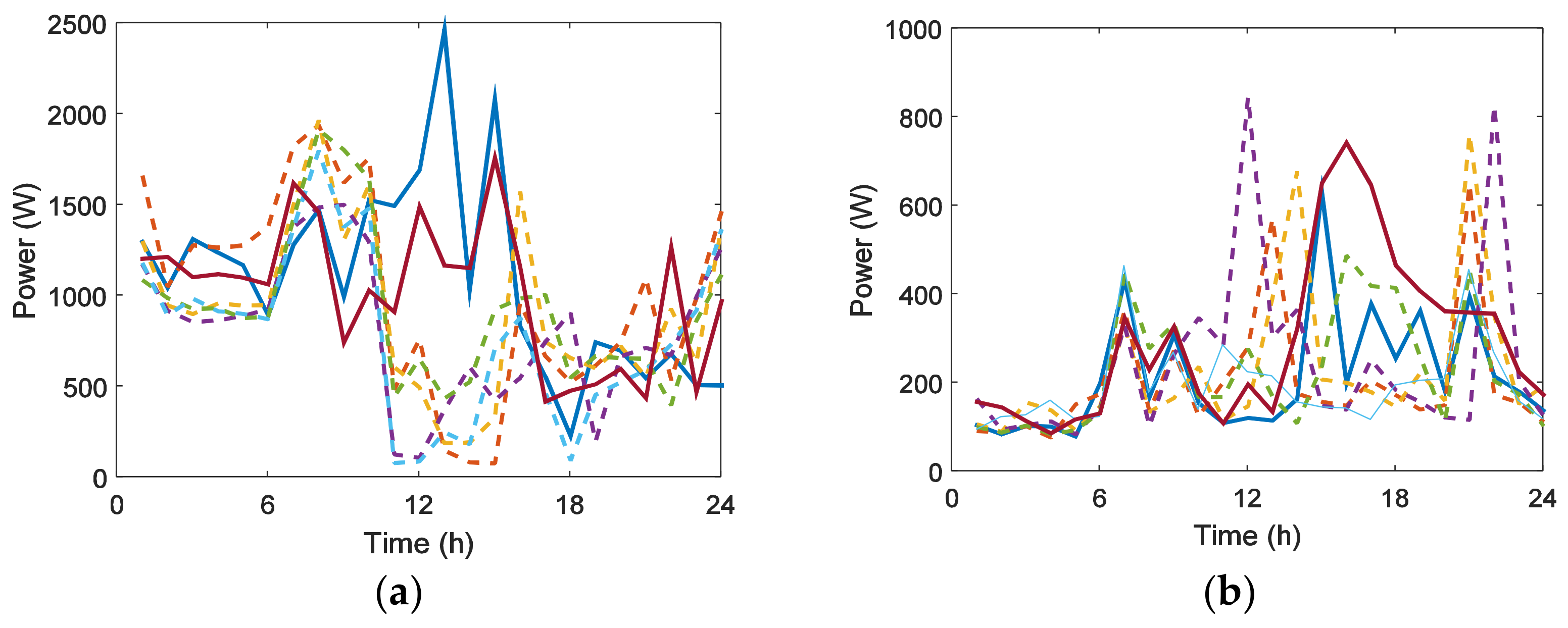Figure 5 shows some examples of daily load curves.

The main end-uses are presented in

Table 1. Customer’s main end-uses and their power.

End-Use	Description	Power (kW)
HVAC	Heat Pump/Air Conditioning (inverter) split unit 3300 kcal/h	[0, 1]
WH	Water heater, 80 L capacity	≈2
SH	Convection electric heater	≈0.6, 1 or 2
RF	Refrigerator/freezer	0, 0.1 or 0.3
EA	Electronic appliances: TV, DVD, PC, etc.	[0, 0.5]
L	Lighting	[0, 0.3]
WM	Washing machine	[0.1, 0.45]
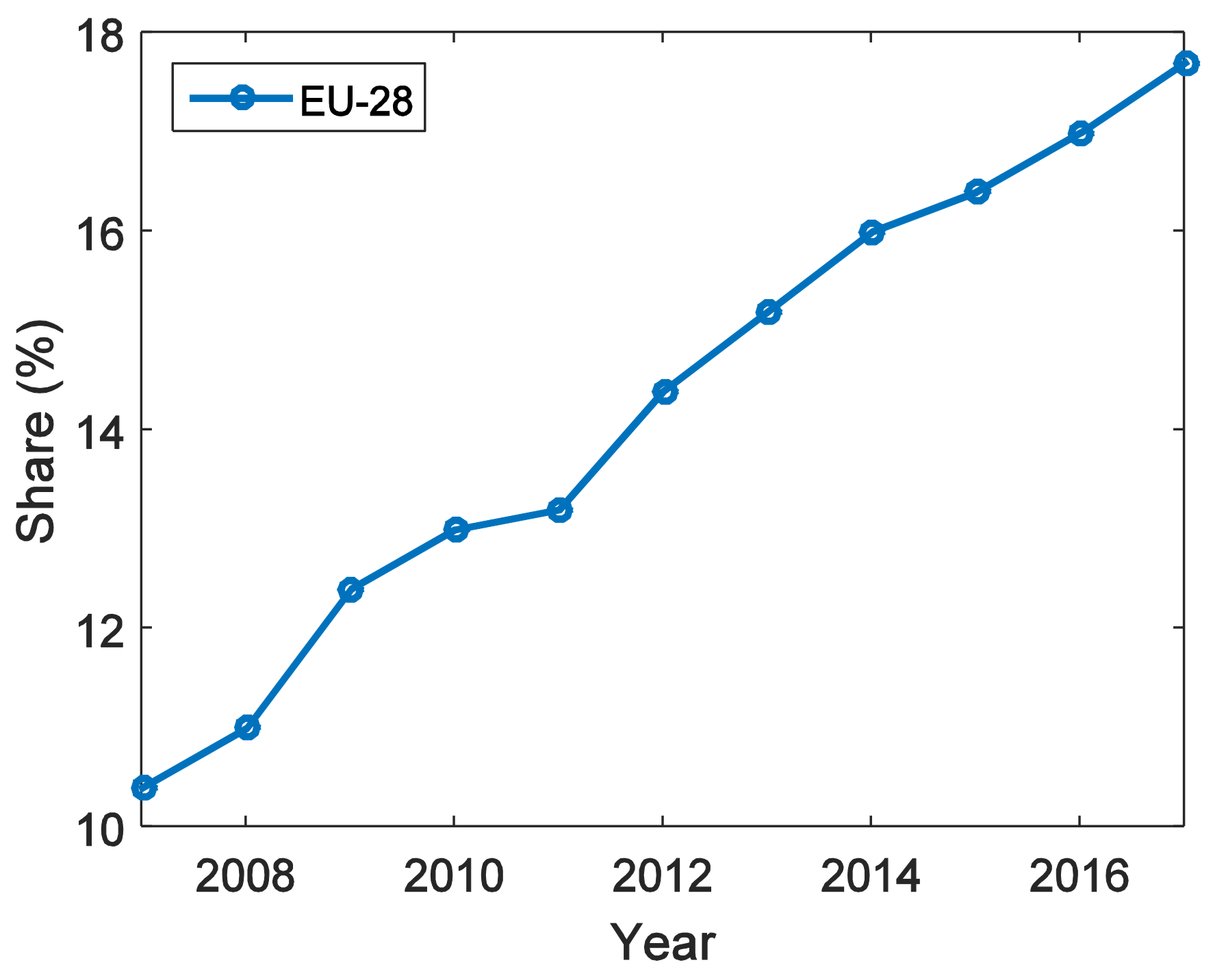
COK	Cooking	1 or 2

(note that some end-uses exhibit a few discrete states in demand while others have a wider range of values). To demonstrate that both the validation scenario and the residential customer are representative, typical household end-uses database in the European Union EU-28 [13] and in the USA [35] have been considered. According to low levels of penetration of renewable solar systems in buildings [36] (i.e., solar heat pumps and solar water heaters), electric supply has been considered as primary source for these end-uses. Several analysis in the literature state that end-use renewable solutions are perceived of as innovative and risky, and the average customer requires higher rates of return than for more conventional systems [36] (notice that the same concern appears for Energy Efficiency measures such as the replacement of conventional WH by Heat Pump WH).

Table 2. Main End-Uses share in the residential sector according to some estimates in the USA [35], EU-28 [13], and Spain [38].

Type of End-Use	USA (2009) All Fuels	USA (2009) Electricity	EU (2016) All Fuels	Spain (2014) All Fuels	Spain (2014) Electricity
Space Heating	41.5	9.3	64.7	42.9	7.36
Water Heater	17.71	9.75	14.5	17.9	7.47
Air Conditioning	6.24	14.47	0.3	0.98	2.33
Refrigerators	4.75	11.03	-	7.94	-
Other *	29.8	55.45	20.5	39.22	82.84

* Appliances and Electronics.

presents the average energy consumption in households (in some cases, the share of end-uses is considered for all types of fuels because it is more representative) in Spain, EU-28, and the USA. Notice that in European Mediterranean climate regions like in the USA southern regions, air conditioning loads represent a higher percent (66% of households have this appliance and the trend is quite solid in this decade: around 700,000 new units in Spain, 80% of them in the residential sector, i.e., 12% of the EU market [37]). The assumption of annual residential percentages (national reports) in the proposed scenario (“prosumers”) could be a critical error for simulation purposes (i.e., DR potential being considered in summer periods, when solar resources and HVAC peak).

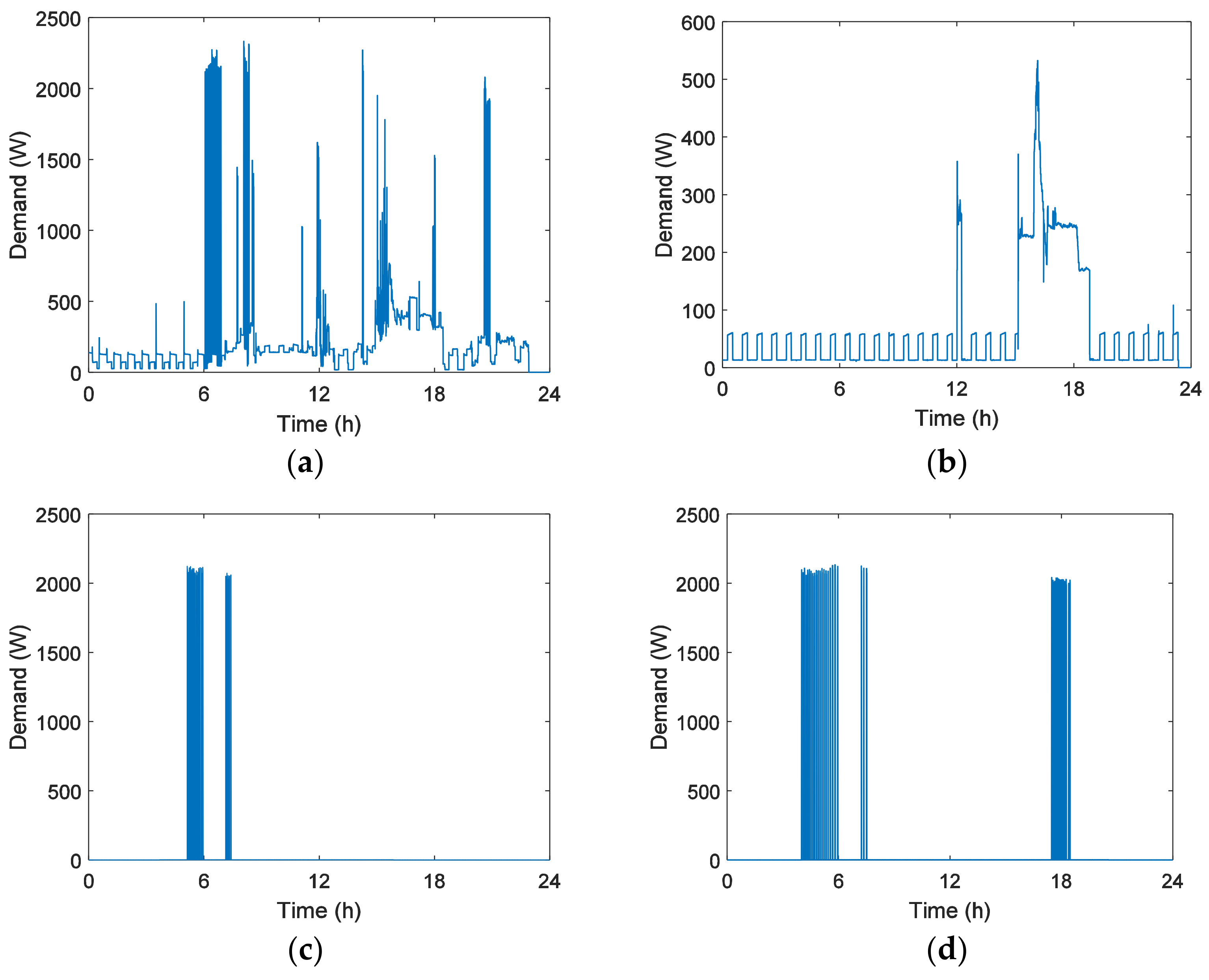
Figure 6 presents the overall demand and the consumption of main residential end-uses in a typical winter day (23 January 2017). During these days, the average daily demand is around 22–25 kWh. The granularity of data is fixed from 10 to 20 s for a better evaluation of end-uses and to achieve a customer database with multiple possibilities (see for example REDD database in a past paper [34]). For example, this database has been tested for Non-Intrusive Load Monitoring Methodologies (NIALM) through Smart Meter data, for different purposes and loads (the use of NIALM for the disaggregation of main loads can be found previously [29] and for small nonlinear loads in a past paper [39]). This pacer, for monitoring purposes, is of considerable interest in the case of some water heaters with fast switching because demand cycling ranges from 10 to 30 s in some periods. Moreover, the continuous or discrete use of electricity, the presence of one or several states for appliances, is a matter of concern for DR, and in this way, a more precise knowledge of end-uses allows an optimal estimation of Load Models and then, a better evaluation of the possibilities of the different policies available on the Demand-Side.

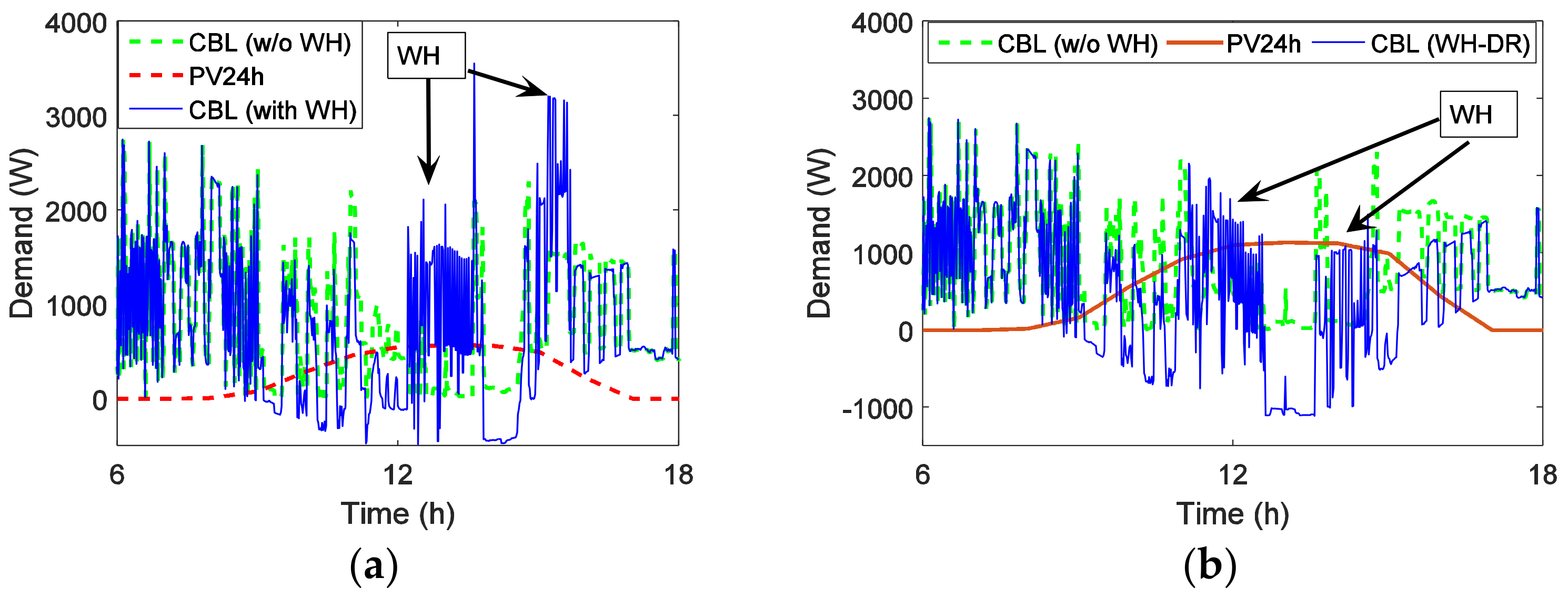
Figure 7 shows the overall demand and the consumption of main end-uses in two typical summer days (12 June and 2 July 2017). For those days, daily demand is around 5–6 kWh (i.e., around 25% of winter demand). The granularity of data is fixed from 10 to 20 s again. In those days, HVAC changes its service to space cooling, and the oil-filled radiator is out of service. Note that our customer has the WH controlled by a timer to take profit of ToU tariffs, but in some cases, the customer disables the timer and control actions. This is an option to take into account for any possible DR control (see Figure 7d). Another aspect to be considered are the loss of customer service and the losses attributable to energy storage loads when the load service (hot water) and demand (electricity to heat conversion) occur with different time lags. This topic is not considered in lots of papers in the literature, mainly interested in optimization concerns of “static” loads which change demand irrespective of service or environmental variables which strongly condition demand, for instance in a past paper [30].

Some additional data of interest from Figure 6 and Figure 7 are shown in

Table 3. Overall demand and Main End-Uses share for the residential customer selected for simulation purposes for two typical days (January and July).

Type of End-Use	Winter (kWh)	Share (%)	Summer (kWh)	Share (%)
Space Heating (HVAC)	9.06	39	NA	-
Water Heater	1.62	7.1	1.15	20.8
Air Conditioning	NA	-	1.52	29
Refrigerators	1.12	5	1.62	31
Space heating (radiator)	6.94	30	NA	-
Overall demand	23.05	100	5.20	100

. A brief comparison between Table 2 and Table 3 shows that loads with storage (implicit or explicit one) such as Space Heating (up to 69% in winter), Air Conditioning (29% in summer periods), and Water Heater (from 7 to 20%) are also the main DR end-uses for the proposed “representative” customer in this study. Moreover, it is interesting to note that refrigerators are of interest too for DR (mainly in summer periods and for Ancillary Services) but its controllability is much more difficult for energy management concerns.

2.2. Solar Resource

In order to know if a location is appropriate to install solar PV systems it is necessary to take into account irradiation levels and other parameters such as modules’ orientation and inclination which influence the systems efficiency.

There are many tools available to estimate solar PV production. In this way, potential prosumers can know what benefits are going to obtain and what environmental impact is foreseen before making a decision about whether or not invest in RES. In the current study, four software packages have been analyzed: PVGIS, RetScreen, HOMER, and SAM.

First, the Photovoltaic Geographical Information System (PVGIS) has been considered [6]. PVGIS is a research, demonstration, and policy-support instrument for solar energy resource, part of the SOLAREC action at the Joint Research Centre of the European Commission. This tool has a large meteorological and solar radiation database accessible to any user.

In order to perform simulations, the latitude and longitude of PV system location and also modules’ material, their orientation and inclination and the availability of tracking structures and ESS are required. Results obtained with this simulator perform a preliminary analysis of solar PV production.

RETScreen [40] is a free software package developed by Natural Resources Canada National Laboratory. RETScreen can make project feasibility analysis and energy efficiency studies from renewable resources and cogeneration as well as ongoing energy performance analysis. The software calculates monthly energy production and exposes the results of an economic, technical, and environmental analysis.

RETScreen cannot make simulations with hourly consumption and only performs a prefeasibility analysis.

HOMER (Hybrid Optimization Model for Multiple Energy Resources) [41] is a software platform that was purchased and enhanced by HOMER Energy. This tool simulates renewable systems operation and optimizes plants design. In addition, HOMER allows including in the same project renewable and nonrenewable energy systems as well as ESS, taking part of micro grids that are studied.

HOMER simulations use meteorological and consumption data from a whole year that can be entered in time intervals between an hour and a minute. Technical and economical results have much more accuracy than RETScreen because of using hourly data instead of monthly averages.

Finally, System Advisor Model (SAM) platform [42] was selected to develop this study. SAM was created by NREL just like HOMER and it is continuously updated by its developers. SAM is a free tool that allows studying RES performance and economic feasibility.

The platform uses a large meteorological database and also a technical database about modules, inverters, and batteries which is available, including systems elements and installation costs. SAM includes links to Utility Rates Database (URDB) from NREL [43] and Database of State Incentives for Renewables & Efficiency (DSIRE) from NC Clean Energy Technology Center [44]. It is also possible to enter your own parameters to perform simulations.

This application uses meteorological and consumption data from a whole year, entering data in time intervals that range from a minute to an hour, the same as HOMER.

The procedure to perform simulations starts by selecting what RES is going to be studied (PV, wind, biomass, geothermal, etc.). Then, a financial model is selected. Available financial models are residential, commercial, third party ownership, and different types of Power Purchase Agreement (PPA).

Once renewable source and financial model have been selected, it is necessary to introduce technical and financial parameters from RES installation, loads (i.e., specifications from modules, inverters, batteries and their configuration, system losses including shading and snow losses, and system costs), financial parameters, and incentives, and finally information about the consumer’s electricity rate and electricity load. Finally, it is possible to make a sensitivity analysis with the main parameters of the renewable system.

2.3. Analysis of Load Flexibility through Physically Based Load Modeling (PBLM)

The flexibility of loads is a main concern to boost the generation from renewable sources on the Demand-Side, specifically for solar resources. The possibilities, for different loads and appliances, to change their consumption patterns to balance intermittent generation have been presented and discussed in previous works in the literature [45]. Another alternative is the use of the sun as a primary energy source for end-uses [36], but this is a complex scenario in the short term. The capability of loads to respond to DR policies depends on load behavior (and its environment) and on the possibility of loads to store energy (service provided). These facts explain that thermostatically controlled loads (TCL) are the most suitable loads for lots of DR policies (i.e., HVAC or WH). An interesting way to evaluate this response is through PBLM, a methodology first proposed by Ihara and Schweppe to solve the so called “cold load pickup” problem [46]. The proposed approach in this section follows the same idea proposed in thermal design software tools such as eQuest and EnergyPlus [47,48]: a white-box model. These approaches sometimes are too complex to evaluate load response in the short term (e.g., EnergyPlus works with high order state-space models, e.g., the model order is approximately 30–40) and they need some simplification to make costs affordable and efforts feasible to engage DR. Some software, for example the toolbox BRCM, is proposed to reduce and simplify the higher order of EnergyPlus models [49] while the toolbox uses the same physical information as the input database (another advantage of white-box approaches) [50].

The advantage of “white box” models as PBLM (or “grey box” according to some authors [51]) is that they allow the user to evaluate the effects of a nonelectrical input/parameter/variable (e.g., the effects of roof and floor insulation, solar radiation levels or the customer service, the changes on water flow q(t) at some established temperature…) to estimate demand changes and energy savings, which is necessary in the case of the implementation of DR policies, or in balancing the volatility of RES (understood as a lack of predictability of the series and not as a time series with a high variance [52]).

Since DR is complex for the demand-side actors (customers and energy aggregators), the philosophy adopted for modeling is to save time, information, and resources and, consequently, use the same modeling basis for different DR policies, markets (Energy, Capacity or Ancillary Services), and loads, whenever possible [53]. This seems affordable with the use of PBLM models because they involve physical information of loads, appliances, and environment. Moreover, the aggregation and validation of these individual models is performed through several tools [29,54].

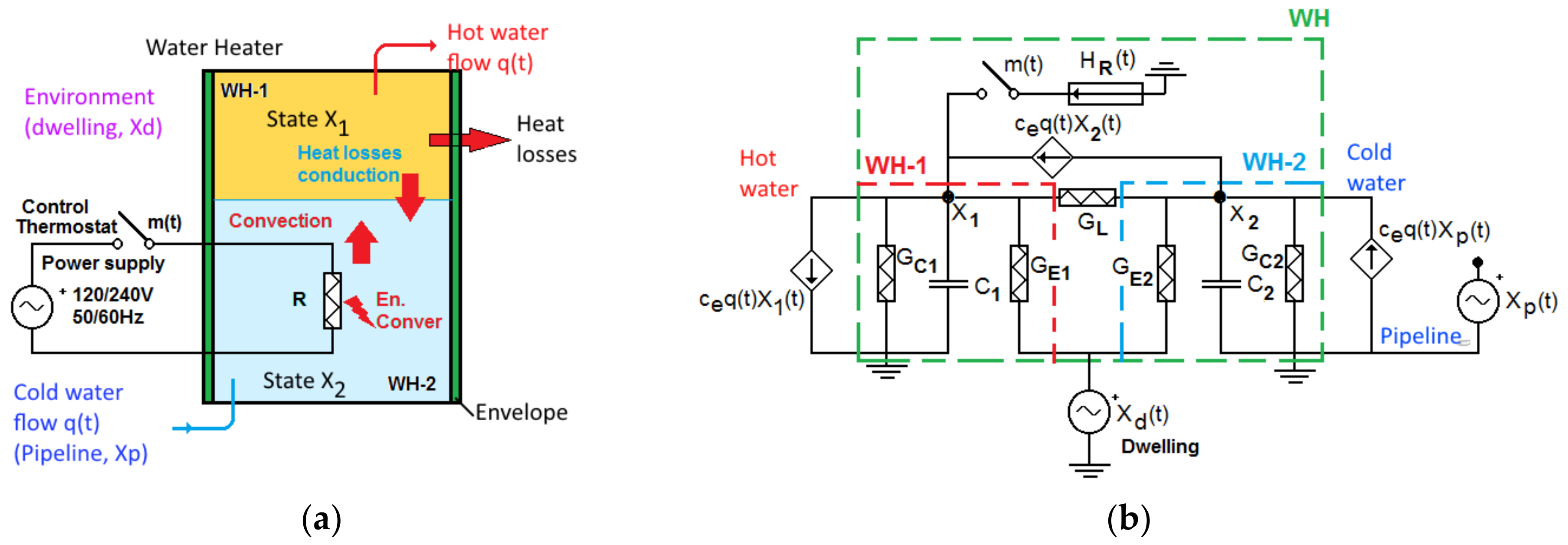
Figure 8 presents the basic steps to build a PBLM model. First, the researcher should find the energy flows on the load (appliance and its environment) and the physical laws that govern these heat flows. For the case of WH, the load needs to supply thermal energy (H_R(t) converted from mains electrical supply, R) to the inlet water flow q(t) (litre per minute) to raise the temperature of the water in the pipeline X_p(t) to the service temperature X_S(t) desired by user inside the water heater (note that due to service conditions, the temperature of water inside WH, X₂(t), may or may not reach X_S(t)). As the temperature of the water increases (water gains energy, at a rate explained by its specific heat c_e and the mass of water stored in the WH, m_w, i.e., usually done in liters or gallons), the load faces losses through the external envelope and the pipelines (h, thermal transmission coefficients or U values) that cross outside the WH tank. The energy balance Equation (hot water energy service equals net energy inputs minus losses) can be expressed by:

$$\begin{array}{l}Service:\frac{d}{dt}\left[m_w{c}_e(X_S(t)-X_p(t))\right]\approx c_{e}q(t)(X_2(t)-X_p(t))\\ En.Input:H_R(t)-Storage-Losses=H_R(t)-c_e{m}_{ws}\frac{d{X}_2(t)}{dt}-h(X_2(t)-X_d(t))\\ Control:m(t)\{\begin{array}{c}m(t+\Delta t)=m(t);x_i<X_2(t)<x_s\\ m(t+\Delta t)=1;X_2(t)<x_i\\ m(t+\Delta t)=0;x_s<X_2(t)\end{array}\end{array}$$

(1)

These equations are translated to a thermal-electric equivalent to make more homogeneous the further and necessary aggregation of individual models, for instance, to achieve a minimum level of load to participate in energy markets [55,56]. These PBLM models usually have several components (sub-models), for example:

-

Load/environment: parameters that represent heat losses/gains (conduction/convection through the external envelope: G_E1, G_E2; the pipeline: G_C1 and G_C2). Also, the model takes into account heat storage from the specific heat of water (C₁ and C₂).

-

The appliance: and its energy conversion into hot water. This is represented by a current source (H_R) and is independent of the kind of WH (standard or Heat Pump Water Heater, HPWH).

-

Control mechanisms (one or several) which drives the demand: a thermostat in some loads, i.e., m(t) in Figure 8b.

-

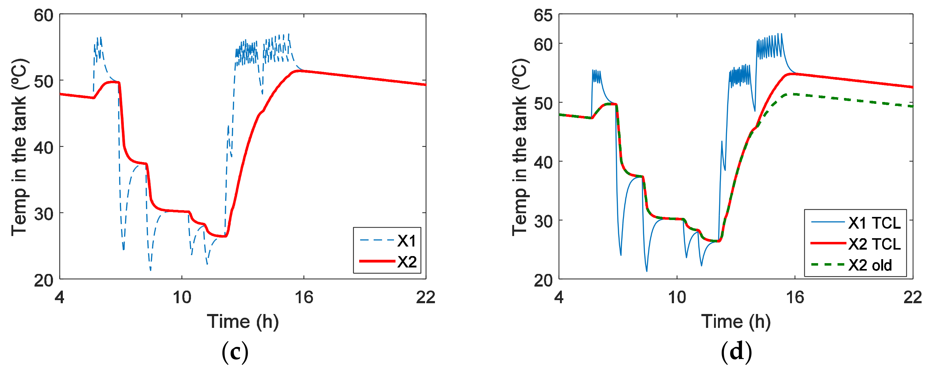
The state variables that usually are temperatures: the temperature of the water inside the virtual subtanks WH-1 and WH-2 (X₁) and (X₂), as shown in Figure 8b. In this case two tanks have been considered to account for the stratification phenomenon in the tank [57].

-

The service of the load: the water load flow q(t) at a certain temperature level Xs.

These parameters must be evaluated through measurements, the application of physical concepts, inspection on-site, and data from the manufacturer. Comparison of the pre and post calibration model shows that a calibration process in white-box models greatly improves the model’s accuracy for each en use [48,58]. For example, the initial estimation of the capacitance value in the equivalent heat storage (C₁ or C₂) can be evaluated by:

$$\begin{array}{l}C=C_1+C_2=V\rho c_e=(80\mathrm{l})(0,99\mathrm{kg}/\mathrm{l})(4.18\mathrm{kJ}/\mathrm{kgn}\mathrm{n}K)=331\mathrm{kJ}/\mathrm{n}K\\ H_R(t,X)=P_R^{avg}COP(X_d,X_1)\approx 2000\ast 1.0=2000\mathrm{J}/s\end{array}$$

(2)

where: V is the volume of the WH tank, ρ is the water density (from 0.998 at 20 °C to 0.983 at 55 °C) and specific heat c_e of water. P_R is the power of resistor (in average) and COP is the coefficient of performance (this is an important factor for WH Heat Pumps).

For instance, state-space representation for the model presented in Figure 8a,b and Equation (1) is:

$$\begin{array}{l}\left(\begin{array}{c}D{X}_1(t)\\ D{X}_2(t)\end{array}\right)=\left[\begin{array}{cc}-\frac{1}{C_1}\left[G_L+G_{C1}+G_{E1}+c_{e}q(t)\right]& \frac{1}{C_1}\left[G_L+c_{e}q(t)\right]\\ \frac{1}{C_2}\left[G_L\right]& -\frac{1}{C_2}\left[G_L+G_{C2}+G_{E2}+c_{e}q(t)\right]\end{array}\right]\left(\begin{array}{c}{X}_1(t)\\ X_2(t)\end{array}\right)+\\ +\left[\begin{array}{ccc}\frac{1}{C_1}{G}_{E1}& 0& \frac{1}{C_1}\\ \frac{1}{C_2}{G}_{E2}& \frac{c_{e}q(t)}{C_1}& 0\end{array}\right]\left(\begin{array}{c}{X}_d(t)\\ X_p(t)\\ H_R(t)\end{array}\right)\end{array}$$

(3)

where D is the differential operator and, coefficients, state variables, and inputs have been previously described (the nomenclature section is at the end of this paper).

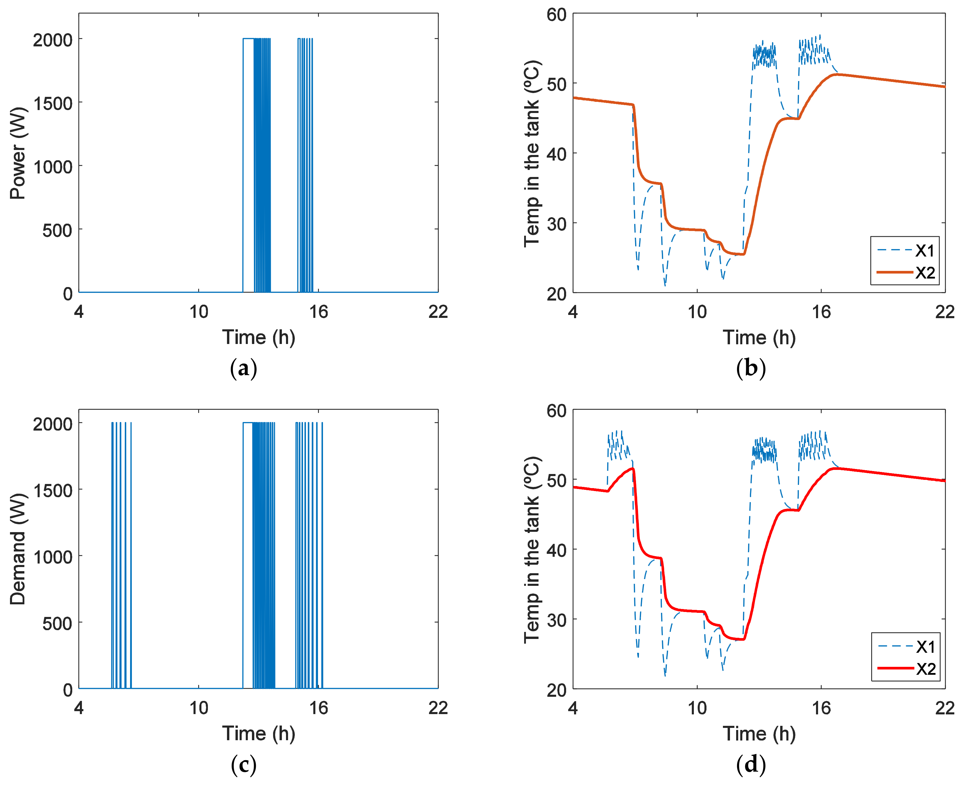
The resolution of state-space system (3) allows the evaluation of thermal losses. This is an important value for the change of WH patterns (as shown in Section 3). For example, system losses through the tank envelope (and WH class, i.e., its energy label) can be evaluated in a period of time T through:

$$Losses={\displaystyle \underset{0}{\overset{T}{\int }}\left(G_{E1}(X_1(t)-X_d(t))+G_{E2}(X_2(t)-X_d(t))\right)dt}$$

(4)

Some other values can be extracted from (3), for example the State of Charge (SoC), the capacity of thermal storage (TESScap), or the Reserve Margin for Storage (RMS, per unit) to store additional energy from operational conditions (i.e., rise the service from X₁, X_S to the maximum thermostat set-point X_S^MAX), specifically:

$$\begin{array}{l}SoC(t)(\%)=\frac{m_w{C}_1\left(X_1(t)-X_p(t)\right)+m_w{C}_2\left(X_2(t)-X_p(t)\right)}{m_w(C_1+C_2)}\left(\frac{100}{\left(X_S-X_p(t)\right)}\right)\\ RMS(t)(p.u.)=\frac{m_w{C}_1(X_S^{MAX}-X_1(t))+m_w{C}_2(X_S^{MAX}-X_2(t))}{m_w(C_1+C_2)X_S}\\ TESScap=m_w(C_1+C_2)\left(X_S-X_p(t)\right)\end{array}$$

(5)

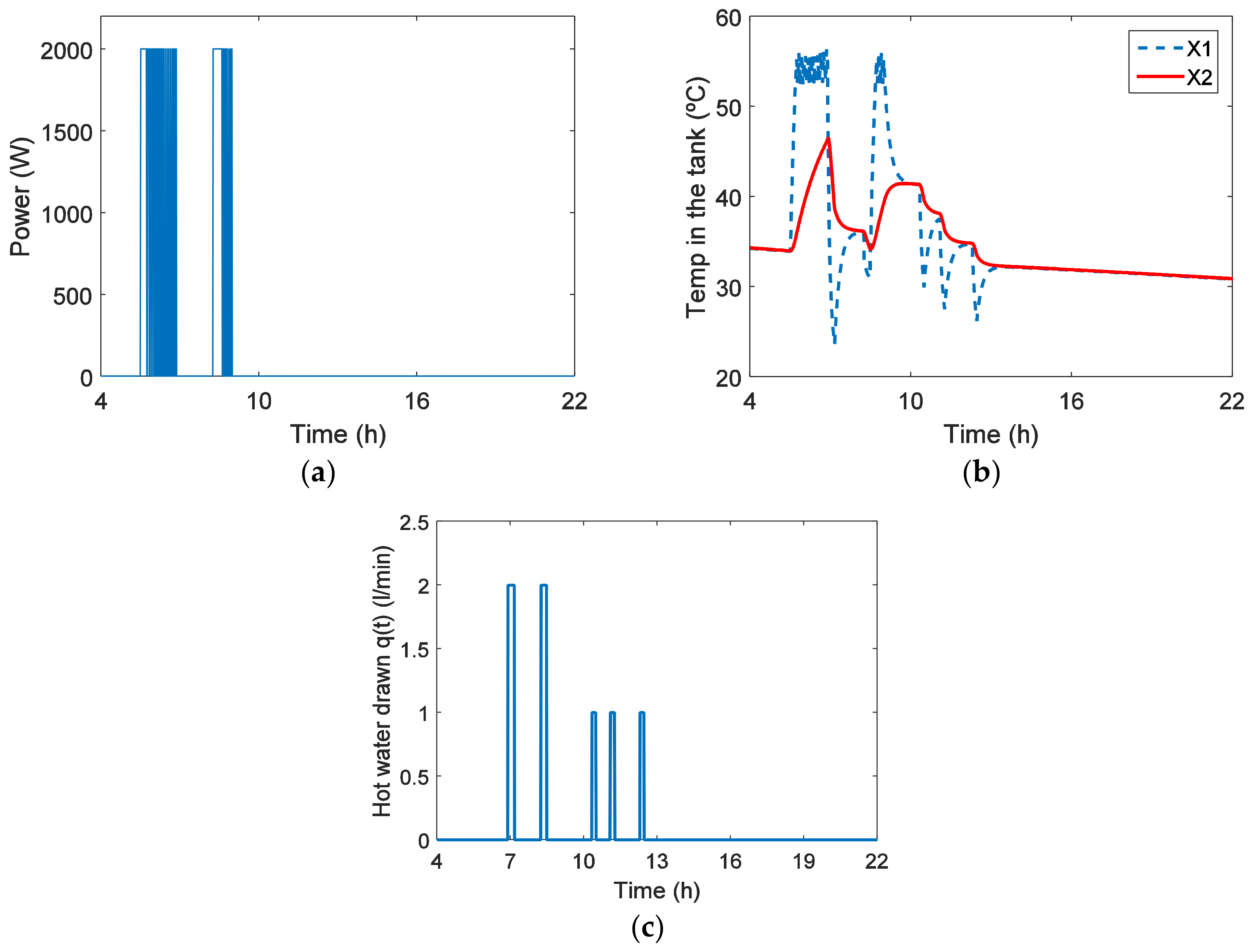
These models (3)–(5) have been implemented in Matlab, validated, and the parameters have been calibrated through several measurements in individual customers: for example, a start-up test (for the evaluation of the stratification of water inside the tank and definition the size of subtanks, see Figure 8a) with the tank in a certain state of charge (SoC, i.e., hot water temperature at the beginning of the test), standby-tests and some tests with several service levels, i.e., different water draws q(t). Another approach to identify the entries of matrices in Equation (3) of PBLM models is to develop a regression problem [50], i.e., a nonlinear optimization problem that involves multiplication of the variables (the model parameters). Authors observed in a past paper [50] that if the dataset is small, the regression problem can lead to an unstable bilinear model. This can be overcome by the evaluation of initial values in (3) from a physical evaluation of the thermal processes in the load and its environment.

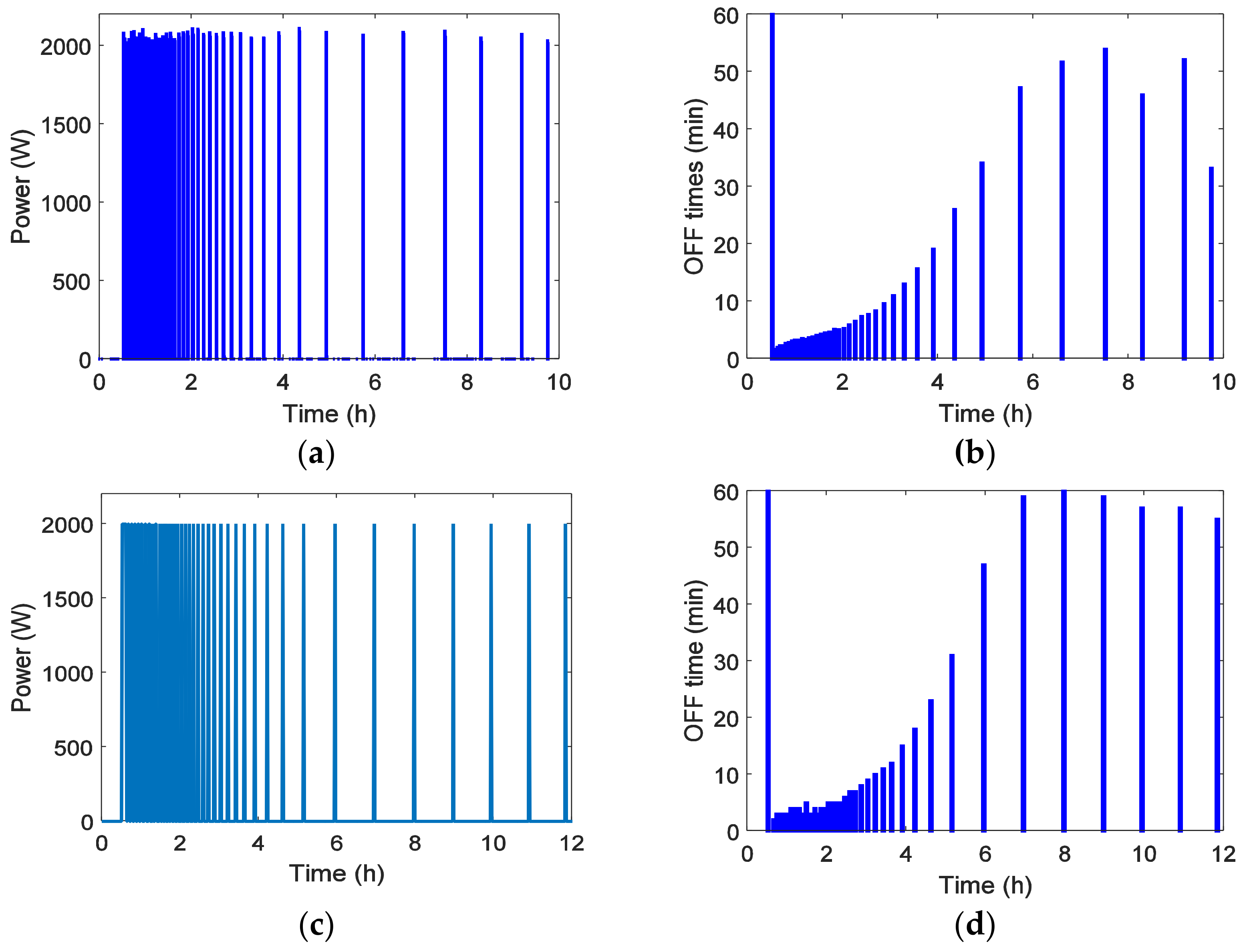
Figure 9 shows the standby times of the test appliance and its model. Appliance switching times between ON periods are around 50–55 min and show an small difference with the model but, in this case, the energy consumption during the start-up and the standby modes is more important for calibration [48] and validation purposes (an average demand around 30 Wh/h in standby for the model and from 27 to 33 Wh/h in the real tests, time periods from 6 h to 10 h are shown in Figure 9a. The consumption during charge (from 0 to 4 h) is 1.65 kWh in the real test, and 1.52 kWh for the simulation model, i.e., around 8% of error, mainly attributable to the stratification of water inside the tank and the accuracy of the control mechanism, i.e., the thermostat, m(t)).

2.4. Balancing PV Generation and Flexible End-Uses in the Demand-Side

In some scenarios, for example in Spain, and from the point of view of the customer, it is interesting to maximize the load that is covered by PV resources because the injection of energy to the network lacks of interest (i.e., the system apply charges to energy injected to the grid, making each kWh self-consumed more profitable than each kWh sold in the market), otherwise the customer gives free PV energy to the system, see Section 1.2). For this reason, it is interesting for the customer to modify the time-of-use of some loads, for example the pattern of WH demand.

In this case, the aggregator or the energy supplier can provide some estimation of WH end-use (see Figure 6) through NIALM [39,54]. The methodology proposed here is to lag or lead the end-use profile of WH, taking into account the changes on demand and customer service, to optimize a specific value, for instance: minimizing net demand, maximizing or minimizing the PV injection to network, minimize the costs of tariffs…, or simply to size the number and kWp of the PV array. Figure 10 shows the lag of WH demand according to two generation sizes: 1 kWp and 2 kWp.

Table 4. Analysis of results of WH lagging (winter period).

PV Array (kWp)	Demand of Customer (kWh)	PV Gener. before DR (kWh, %)	Demand of Prosumer before DR (kWh)	Demand of Prosumer after DR (kWh)	Net PV Injected to Grid (kWh, %)
1	24.75	1.17 (36%)	22.59	22.0	0.58 (17.9%)
2	24.75	3.23 (50%)	21.42	20.06	1.87 (28.9%)

shows some results. From these results and scenario, 1 kWp is a better option for the customer than 2 kWp (taking into account the Spanish Regulation framework).

2.5. Economic Analysis

For this study, two benchmarking tools have been considered to evaluate the cost-effectiveness of the project: Payback time and Levelized Cost of Electricity.

Payback time is a simple method to study the adequacy of the investment and represents the number of years before the system begins to generate some profit.

$$Paybacktime(years)=\frac{System\cos ts(currency)}{Annualprofits(currency)}$$

(6)

Levelized Cost of Electricity (LCOE) is a financial parameter used to assess feasibility and cost-effectiveness of different generation sources on a consistent basis [42]. Usually, it is used to compare renewable energy generation with traditional technologies. LCOE is calculated as the sum of the total lifetime cost of producing electricity with the system divided by the total estimated energy generated from the system over its lifetime. That is depicted in Equation (7):

$$LCOE=\frac{C_0+{\displaystyle \sum _{n=1}^N{C}_n{(1+d)}^{-n}}}{{\displaystyle \sum _{n=1}^N{E}_n{(1+d)}^{-n}}}$$

(7)

where C₀ is the initial investment costs; C_n are the annual project costs including operation and maintenance (O&M) expenditures in year n; d is the discount rate; E_n is the energy (kWh) generated by the system in year n; and N is the investment analysis period in years. LCOE results are expressed in price per kWh, in this case in €/kWh.

LCOE represents the total project lifecycle costs and it can be understood as the price at which total energy generated by the system must be sold to make it profitable during its lifetime.

2.6. Environmental Analysis

One of the most important benefits for increasing renewable generation is the reduction of GHG emissions. Some impact indicators have been used in order to be able to measure the impact of renewable systems and their associated emissions during their life cycle, known as Life Cycle Assessment (LCA).

Life cycle of solar PV systems starts obtaining raw materials and includes all phases of manufacturing, transporting, and installing the system. Also, it is necessary to include the energy used to manage and recycle all the elements at the system end of life.

For this study, Energy Payback Time and Energy Return on Investment have been selected to analyze the life cycle environmental impact from solar PV systems.

Energy Payback Time (EPBT) is defined as the period required for a renewable energy system to generate the same amount of energy (in terms of primary energy) that was used to produce and recycle the system itself [59].

$$EnergyPaybackTime=\frac{E_{mat}+E_{manuf}+E_{trans}+E_{inst}+E_{EOL}}{\left(\frac{E_{agen}}{{\eta }_G}\right)-E_{O\&M}}$$

(8)

where:

• E_mat: Primary energy demand to produce materials comprising PV system;
• E_manuf: Primary energy demand to manufacture PV system;
• E_trans: Primary energy demand to transport materials used during the life cycle;
• E_inst: Primary energy demand to install the system;
• E_EOL: Primary energy demand for end-of-life management;
• E_agen: Annual electricity generation;
• E_O&M: Annual primary energy demand for operation and maintenance;
• η_G: Grid efficiency, the average primary energy to electricity conversion efficiency at the demand side.

The sum total of the (renewable and nonrenewable) primary energy harvested from the geo-biosphere in order to supply the direct energy (e.g., fuels and electricity) and material (e.g., Si, metals, and glass) inputs used in all its life-cycle stages is known as the life-cycle cumulative energy demand (CED) [59] and corresponds to the numerator of the Equation (8).

Energy Return on Investment (EROI) is calculated by dividing system lifetime period between EPBT. EROI can be calculated using the following equation:

$$EROI=T\frac{\left(\frac{E_{agen}}{{\eta }_G}\right)-E_{O\&M}}{E_{mat}+E_{manuf}+E_{trans}+E_{inst}+E_{EOL}}$$

(9)

where T is lifetime period in years and the other parameters match those defined for EPBT.

EROI is a dimensionless ratio that indicates how much energy is obtained from a system of an energy source compared to how much of that energy is required to create and implement the system [60]. EROI also can be understood as the amount of primary energy which is returned to society (i.e., preserved for alternative uses) per unit of primary energy invested in PV, in reference to the current grid mix [61]. If EROI is greater than 1, then the energy production over the PV-system lifetime is larger than the initial energy investment in the manufacturing process [62].

For both indicators, to obtain clear results it is mandatory to choose the approach that most accurately describes the systems parameters and to specify the approach on which the calculation is based. Thus it is necessary to specify the reference electricity mix [58].

There are two existing conceptual approaches to calculate both parameters. The first approach includes using, in the power grid mix, renewable and nonrenewable sources, and understanding PV systems as replacements of all the energy sources used in the power generation mix. The second approach only takes into account nonrenewable sources, understanding PV systems as replacements of nonrenewable energy sources used in the power grid mix.

For this study, parameters of the Spanish 2017 generation mix (electricity from renewable and nonrenewable sources) have been used as reference scenario.

For the calculations of LCA, the information obtained from Ecoinvent database has been used [63] and adapted to specific operating conditions relating to the case of study.

2.7. Electricity Rates and Incentives

Two main type of electricity rates are available for residential consumers (notice that at present the direct access to market and to advanced time-based programs such as real time pricing are scarce or not eligible for these segments [64]): flat rates, which have a constant price for energy consumption throughout the day and Time-of-Use (TOU) rates, in which the price of energy demand depends on the time of the day at which is consumed. TOU used in this study has two periods: peak (between 12 a.m. and 10 p.m. in winter and between 1 p.m. and 11 p.m. in summer) and off-peak (the rest of the day). Prices used to carry out this analysis are presented in

Table 5. Electricity rates for residential consumers.

Tariffs	Prices
	Fixed Charge (€/month)	Variable Charge (€/kWh)
Flat rate	16.45	0.179826
TOU rate	16.45	Peak 0.245829	Off-Peak 0.126133

and include all Spanish taxes.

Three regulation scenarios from RES have been studied as explained in Section 1.3: Net Metering (NEM), Feed-in-Tariffs (FiT), and lack of incentives (LoI), based on regulations from California, Germany, and Spain. Support measures considered in this work are shown in

Table 6. Scenarios for Renewable Energy Sources regulations: incentives.

Scenario	Incentives
NEM	Sell rate at end of year: 0.02373 €/kWh Investment Tax Credit (ITC): 30%
FiT	FiT for energy send to grid: 0.122 €/kWh
LoI	-

for each scheme.

2.8. Financial Parameters

The main financial parameters used for the calculation process are presented in

Table 7. Financial parameters.

Financial Parameters	Value
System costs (including installation)	2.54 €/W
O&M costs	1.5% of capital costs
Lifetime	25 years
Discount rate	1.5%
Inflation	2%
Tariff inflation	2%

. The values of these parameters are based on the literature review [65,66,67,68].

System costs are based on NREL research and include the cost of all required elements: PV modules, inverter, panels’ structure, cabling, etc. Also the permitting and environmental studies, the installation labor, the grid connection, the installer margin, and sales tax (21% of total costs in Spain) are included. The lifetime is fixed in 25 years because it is the performance duration warranty offered by PV modules manufacturers. Inflation and tariff inflation have been selected taking into account the long-term target of the European Central Bank (ECB) to maintain the inflation rate close to 2% [69]. Finally, the value of the discount rate is related to interest rates for long-term government bonds accordingly to the European Central Bank (in 2017, the interest rate in Euro area is ranged between 0.19% and 7.17%) [70]. According to 2017 statistics, 1.5% is selected as the average value in Spain.

3. Results and Discussion

In this section, some simulation results are presented and discussed, taking into account the methodologies considered and developed in Section 2. First, the cost-effectiveness of the conversion from customer to prosumer, without any action in demand, will be presented. Second, the influence of electricity tariffs and regulation scenarios for PV systems will be analyzed, again without DR policies. Then, the advantages of demand-responsiveness for the improvement of customer benefits will be underlined. Finally, other inputs such as environmental concerns are presented because they can also be a driver to engage RES [33].

3.1. “Static” Prosumer: Without DR and ESS

The first case of study represent a prosumer who installs a 1 kW PV system to cover his/her demand (partially) and injects the surplus to the grid. The prosumer, called as “static prosumer”, does not take any other action to improve the system’s performance such as installing EES systems or changing his/her consumption routines. Results from simulations over the three policy scenario studied are shown in

Table 8. Economic results for static prosumer with flat rate.

Scenario	Net Savings (€/year)	Payback Time (years)	LCOE (c€/kWh)
NEM	294	6.1	9.66
FiT	273	9.1	12.42
LoI	200	12.1	12.42

. A flat tariff is considered for the calculations because prosumer is not involved in any DR strategies (including flexible tariffs).

The installation of a 1 kW PV system located in Cartagena, Spain, has an annual energy yield of 1743 kWh/kW and contributes to reduce the electricity bill by €200 per year and can reach almost €300 per year if NEM policies are applied in combination with ITC. Payback time varies between 6 and 12 years and LCOE is found between 12.5 and 9.6 cent€/kWh. In all cases NEM scenario obtains the best results, with the highest net savings and the lowest payback time and LCOE. These results are in agreement with other recent studies from Italy [16] and Greece [17].

3.2. Influence of Electricity Tariffs on the Profitability

Secondly, the influence of electricity tariffs on the profitability of the system is studied. Simulations have shown that the total energy consumed by the loads supposes a total annual cost of €936 if flat rate is the default option. However, if the TOU rate is available, the total annual cost is reduced to €883. This means an annual saving of €53 is achieved for changing the electricity tariff. In addition, net annual savings for PV system with TOU tariffs are greater than with the flat tariff. Therefore, the TOU rate payback time is lower than for the flat rate. The economic results for the simulations of both options are presented in

Table 9. Comparative of economic results between Flat rate and TOU rate.

Scenario	Tariff	Net Savings (€/year)	Payback Time (years)	LCOE (c€/kWh)
NEM	Flat rate	294	6.1	9.66
	TOU rate	348	5.2
FiT	Flat rate	273	9.1	12.42
	TOU rate	300	8.2
LoI	Flat rate	200	12.1	12.42
	TOU rate	235	10.4

for the three regulation scenarios we are dealing with in this paper.

Net savings increase by €27–54 per year applying TOU rates. LCOE results are not affected by electricity tariffs, but using TOU tariffs can reduce payback time between 1.7 years for Lack of Incentives scenario and 0.9 years for NEM and FiT scenarios.

Results obtained with a TOU rate can be compared with a recent study published for Portugal [20]; a country located in the Iberian Peninsula which has similar irradiation levels and electricity prices.

In a past paper [20], similar policy scenarios have been analyzed using a TOU rate with two similar periods (Peak and Off-Peak). The LoI scenario (named as “SC”) for 1 kW system obtains a LCOE value of 14 c€/kWh and 10.89 years for payback time. The NEM scenario (“SC + NM”) results show a payback time of 8.26 and a LCOE of 10 c€/kWh. All these results are similar to those obtained in current work. However, it is necessary to point out that payback time for NEM is lower in the present study than in a past paper [27] due to the 30% ITC. Finally, [20] also studied a FiT scenario (“SC + IN”) with an LCOE of 11 c€/kWh and payback time of 12.89 years. Again, payback time for the Portuguese case is higher than current FiT scenario, but in this case the reason is that authors of a previous work [27] consider a FiT rate based on wholesale market electricity prices (average of 0.052 €/kWh in 2017), which are much lower than the 0.122 €/kWh selected by this study (notice that Wholesale Markets are closed to Residential segments in practice [15,27]).

3.3. “Dynamic” Prosumer: WH as Thermal Energy Storage System

Finally, a prosumer who is able alone or with the support of an energy aggregator, to apply DR strategies has been analyzed, the so called “dynamic prosumer”. A conventional electric WH (heating by a resistor) has been considered, and, in some of the proposed cases, it performs like a Thermal Energy Storage System (TESS). Several cases have been analyzed: first a customer without any kind of PV generation (i.e., the baseline for the study, described in Section 2) which manages demand according to ToU tariffs; second a customer which installs PV and changes WH demand with a simple procedure (a digital timer to control load switching); and, finally, a “dynamic” prosumer that manages demand to follow, to some extent, PV generation. In this last case, the water is heated during the period with the highest solar energy production (or when some PV surplus has been forecasted) to take advantage of the solar resource while minimizing the energy injected to network (see Section 2.4). In this way, the customer avoids generation charges. Hot water is stored and maintained at a set-point temperature (X_S, see Section 2.3) in order to be used when necessary. The problem with this alternative is heat losses during the storage period (due to the necessary delay between storage and water drawn, as will be shown in this paragraph).

Before making any change on end-uses from an economic point of view, it is necessary to account for the service that the customer gets from load, in this case the hot water demand along the day and specially the temperature of water outlet. It is necessary to remark that demand is not a static vector of values, as proposed in some optimization papers [30]. Since the beginning of Demand-Side management policies, the customer experience of DR policies has been disappointing, especially in the past. So, it is basic to achieve customer acceptance of DR for attaining a better engagement of customers in new markets [14], because at present DR is basically a portfolio of customer (aggregator) driven policies. Figure 11a shows the simulated WH end-use “baseline profile” corresponding to a winter day (see also real data in Figure 7c) and the service of the load: temperature of hot water in the outlet (Figure 11b) and water flow drawn (Figure 11c). It can be seen that the end-use “baseline” demand covers the needs for hot water during the day for the residential user (some shower and some housework tasks before lunch time). Moreover, the user switches on the appliance very close to its time of use to minimize heat losses (around 30 Wh per hour, as explained in Section 2.3). Notice that this section estimates that the overall water drawn, according to individual demand of WH, is around 80 L/day and that the system use mixing valves to maintain and limit mixed hot water (temperature X₂) to a desired and selectable temperature (for example, during a shower, water flow can get up to 10 L/min of mixed water [71], that is to say, the customer uses approximately 120 to 140 L/day of mixed water).

Figure 12 shows the effects of a change in the end-use pattern of WH to achieve the maximum profit from the green energy available (surplus) from the PV array (according to the methodology that was presented in Section 2.4). Figure 12a presents WH demand (the same individual demand of Figure 11a but with a delay of 6.5 h from the morning to the afternoon, to tune the elemental demand with PV surplus, see Figure 10b). The effect of this delay (again through a timer) is that the first water drawn (and heat losses) decrease the temperature of the tank to 34 °C and this makes it more difficult to maintain service until the next recharge of reservoir. The solution is depicted in Figure 11d: an additional switching-on of the appliance is planned (out of patterns considered by black-box models) for at least 30 min (0.3–0.4 kWh) in the early morning to recover a minimum service during the next shower (see Figure 11c,d, where water temperature grows approximately 3–4 °C with respect to Figure 11b). Notice that a water temperature from 22 to 27 °C is considered cold water [71] and has some effects on the human biology, whereas 28–30 °C is considered a minimum standard of quality for moderately warm water in dermatology.

Finally, a new test has been performed through PBLM models. It is considered that the customer allows a third party (an automated system or an aggregator) to change patterns and tune demand (ON/OFF cycling) according to the energy generated by the PV array to take the maximum profit from PV generation and avoid the injection to the Power System (values for PV injection can be seen in Table 4). Figure 13a shows the results in the overall curve of the prosumer where HW covers PV surplus in the early afternoon (see Figure 10a). Figure 13b shows the new WH pattern, with the same problem as in the previous case, the appliance needs to recover heat losses in the period from 3 p.m. to 6 a.m.

The PBLM model deals with an additional concern in practical situations: the WH reached the service temperature and goes to off state (or WH performs ON/OFF cycles with a demand lower than foreseen, see for example Figure 9b, which entails a low capacity of consumption/response) or in the case that the PV generation is above the predicted values. In this case, the model allows the aggregator to define a change in thermostat set-point to force a higher switching rate and, consequently, an increase in demand (in a similar way that HVAC load can perform during preheating and precooling periods but with fewer heat losses) to increase the state of charge of WH, using the tank as TESS or like an EES (i.e., a battery, but with lower capital or maintenance costs for the customer). Figure 13d shows the results in the internal temperature of the tank: an increase around 5 °C (Xs was fixed at 55 °C, but standard WH allow set-points up to 62–65 °C, i.e., the customer still has a RMS of around 13%). From a technical point of view it is not very difficult to perform these tasks through home automation software and hardware [54]. Numerical results in

Table 10. Technical (demand/generation/service) results for the different prosumers.

Case	State of Charge (max, min) °C	Demand of Prosumer (kWh)	WH Service (Shower) (°C)	Net PV Injected to Grid (kWh, %)
Baseline (two period tariff but without DR)	47, 31	22.0	34	1.17 (36%)
Change of WH ToU (time of use)	46, 25.5	22.30	27.5	0.58 (17.9%)
Change of WH time of use + “preheating”	49, 27	22.63	31	0.58 (17.9%)
Change of thermostat settings	55, 27	22.66	31	0.30 (9.3%)

provide a better estimation of performance (both for energy and service level) in the different cases. The baseline case performs well from the point of view of WH service, but wastes 36% of the renewable energy available. The change of time-of-use of the WH pattern recovers a half of the PV energy wasted previously, but has two important drawbacks: the service of WH (a minimum SoC of 25 °C) requires an increase of demand to recover energy losses (the hot water must be stored during 16 h until the next service). Finally, the dynamic change of the thermostat proposed in this subsection entails the best results: the PV injection to the grid decreases and there is not any need to recover heat losses anymore (a higher temperature of water maintains service levels until next shower, without an additional demand from the network).

It is also interesting to consider the results of the simulations from an economic point of view for the “dynamic prosumer” that matches demand and supply. These results are shown in

Table 11. Economic results for dynamic prosumer with TESS and TOU rate.

Scenario	Net Savings (€/year)	Payback Time (years)	LCOE (c€/kWh)
NEM	367	4.9	9.66
FiT	337	7.4	12.42
LoI	292	8.5	12.42

. A TOU rate is used for the calculations according to the DR strategies applied.

The use of demand-side flexibility (DSF) in WH consumption allows an increase of the selfconsumption rate from 62% to 66.5% (4.5%) and reduces the energy surplus by 37.8%. Also, DSF involves a reduction of payback time in all cases.

The scenario which obtains the best result is LoI regulation, where payback time is reduced almost 2 years (from 10.4 to 8.5); increasing net savings by €57 per year. In the NEM scenario, net savings increase by €19 per year, reducing payback time from 5.2 to 4.9 years. Finally, FiT regulations complemented with demand-side flexibility obtain a revenue of €337 per year for net savings, increasing by €37 compared to results without DSF, and reducing payback time from 8.2 to 7.4 years.

3.4. Enviromental Results

As it has been stated before, the 1 kW PV-system is located in Cartagena, Spain, one of the cities with higher irradiations levels in Spain, near to 2200 kWh/m² year. The first year energy output for the installation is 1708 kWh and the total lifetime energy output is 39,250 kWh, considering a linear power degradation of 0.7%/year according to the guidelines of IEA PVPS task 12 (20% after 30 years) [72]. The module efficiency and performance ratio are obtained from SAM databases, taking values of 19% and 80%, respectively. Environmental impacts related to operation and maintenance were considered negligible. Grid conversion efficiency (η_g) of 0.416 is used for Spain according to a past paper [73]. The life-cycle cumulative energy demand (CED) adopts a value of 29,107 MJ/kW (5821.4 MJ/m² module). This value is similar to other values found in the literature [61,74,75,76].

Finally an EPBT of 1.97 years is obtained, which means that in less than 2 years PV-system can generate all energy necessary to produce and recycle itself. Assuming a lifetime of 25 years, EROI adopts the value of 12.69. Because EROI is greater than 1, it is possible to say that there is an environmental benefit using the PV-system.

Results obtained in the current study are in agreement with a past paper [76], which obtains an EPBT near to 2 years for an installation in Southern Europe. The authors of a previous paper [62] obtained, for Europe installations of mono-Si modules, an EPBT of 1.9 years and an EROI of 16.1 years. EPBT value is mostly the same that it is obtained in this study, but EROI is greater in [62] because it have been used a lifetime of 30 years.

Finally it is remarkable that Garcia-Valverde et al. [77] conducted a study for a 4.2 kW standalone installation in Murcia, Spain, only 50 km away of Cartagena. In this case, a 9 year EPBT is obtained. The big difference between their study [77] and the current study is due to the use of a battery ESS for the standalone system. Lead-acid batteries have been used. This technology has a maximum lifetime of 10 years and their construction and recycling processes are the energetically and environmentally most expensive. This is the reason why the EPBT increases up to 9 years for this type of installation.

3.5. Limitations of the Methodology

The proposed approach has some limitations: for instance, the need to use NIALM or submetering to tune the parameters of the model. Second, the control of WH; which requires an additional control (not included in conventional WHs) to change conventional WH to TCL. This control involves the need to have a smart thermostat. Fortunately, this technology is available for HVAC (another cheaper option, used for testing in this work, is WiFi or Z-wave thermostats). The randomness of service q(t), mainly in aggregate loads, should be considered in (3) both through Monte Carlo or Stochastic Partial Differential equations (this will be a challenge for the future research). Finally, the volatility of solar resources and the interaction with price-DR, which can change the patterns of the customer, should be considered in a holistic approach.

4. Conclusions

Residential customers can obtain interesting benefits from RES or DR alone, but synergies must be developed to enhance both DR and RES potential and effectiveness. Unfortunately, it is difficult for these segments to overcome some barriers (education and regulation) and manage DR alternatives and PV self-generation, especially in some countries but, in the future, the penetration of RES is foreseen to be more and more important. Moreover, DR potential should increase with the new power mix in the future.

This paper has been focused on the development and synergies amongst different methods (physically based) to help the customer (or its energy aggregator) in the evaluation of benefits when he/she becomes a prosumer. Moreover, the proposed methodology can help to overcome barriers and understand the potential of PV and DR in the short and mid-term, including the active participation in electricity markets; alternatives to be considered in future works. The advantages of the presented approach: The universality of PBLM for load modeling. PBLM takes into account the changes in load profiles due to the change in the time of use (an issue neglected in many optimization approaches), the analysis and consideration of customer service concerns (internal temperature of water), and the possibility of WH to reduce or increase its demand (through the knowledge of its state of charge).

Finally, the paper shows new possibilities for the balance of PV generation through a minimum flexibility of demand, and, in this way, reduces the drawbacks of PV volatility in some periods which would affect power system reliability. The paper also demonstrates, from an economical point of view, that both in appropriate or adverse scenarios, the cost-effectiveness of PV can be significantly improved with the support of DR, specifically the selfconsumption rate rises 25% and payback is reduced around 20% (with respect a scenario without DR). Indeed, the flexibility of demand is of interest: 9–10% at peak. In the future, new opportunities may appear for the customer, but these will require a better management of PV and a more effective DR engagement, and this way, the residential prosumers must be a valuable resource for the management and sustainability of energy in the horizon 2030–2050. For future works, the authors will explore both the possibilities of aggregation and the combination of several loads (for instance HVAC) to increase the selfconsumption rate, gain more flexibility for the demand-side, and improve the possibility of load-generation balance.

References

1. European Commission. Data and Analysis. Indicators for Monitoring Progress towards Energy Union Objectives. Scoreboard. Energy Security, Solidarity and Trust. 2017. Available online: https://ec.europa.eu/energy/en/atico_countrysheets/sco reboard?dimension=Energy+security%2C+solidarity+and+trust (accessed on 13 March 2018).
2. Directive 2009/28/EC of the European Parliament and of the Council of 23 April 2009 on the Promotion of the Use of Energy from Renewable Sources and Amending and Subsequently Repealing Directives 2001/77/EC and 2003/30/EC. 2009. Available online: http://eur-lex.europa.eu/legal-content/EN/TXT/?uri=CELEX:32009L0028 (accessed on 26 August 2018).
3. European Commission. Data and Analysis. Indicators for Monitoring Progress towards Energy Union Objectives. Data and Charts. Decarbonisation of the Economy. Renewable Energy. Renewable Energy Share. Available online: https://ec.europa.eu/energy/en/atico_countrysheets/database?indicator=DE4&type=table&subindicator=DE4-A2 (accessed on 14 March 2018).
4. IRENA. Renewable Capacity Statistics 2018, International Renewable Energy Agency (IRENA), Abu Dhabi. 2018. Available online: http://www.irena.org/DocumentDownloads/Publications/IRENA_RE_Capacity_Statistics_2017.pdf (accessed on 20 August 2018).
5. Eurostat Statistics Explained. Archive: Energy from Renewable Sources. Primary Production of Energy from Renewable Sources, EU-28, 1990–2015. March 2017. Available online: http://ec.europa.eu/eurostat/statistics-explained/index.php/File:Gross_electricity_generation_from_renewable_sources,_EU-28,_1990-2015_F3.png (accessed on 14 March 2018).
6. Photovoltaic Geographical Information System (PVGIS). European Commission. Available online: http://re.jrc.ec.europa.eu/pvg_download/map_index_c.html# (accessed on 21 March 2018).
7. A Roadmap for Moving to a Competitive Low Carbon Economy in 2050, Communication from the Commission to the European Parliament, the Council, the European Economic and Social Committee and the Committee of the Regions, European Commission. 2011. Available online: http://eur-lex.europa.eu/legal-content/EN/TXT/PDF/?uri=CELEX:52011DC0112&from=EN (accessed on 25 April 2018).
8. Energy Roadmap 2050, Communication from the Commission to the European Parliament, the Council, the European Economic and Social Committee and the Committee of the Regions, European Commission. 2011. Available online: http://eur-lex.europa.eu/legal-content/EN/TXT/PDF/?uri=CELEX:52011DC0885&from=EN (accessed on 25 May 2018).
9. Best practices on Renewable Energy Self-Consumption, Commission Staff Working Document, European Commission. 2015. Available online: https://ec.europa.eu/energy/sites/ener/files/documents/1_EN_autre_document_travail_service_part1_v6.pdf (accessed on 21 March 2018).
10. California Public Utility Commission. Available online: http://www.cpuc.ca.gov/General.aspx?id=3800 (accessed on 21 March 2018).
11. ENTSO-E Recommendations to Help Achieve Europe’s Energy and Climate Policy Objectives. 2014. Available online: https://www.entsoe.eu/ (accessed on 19 March 2018).
12. Denholm, P.; O’Connell, M.; Brinkman, G.; Jorgenson, J. Overgeneration from Solar Energy in California: A Field Guide to the Duck Chart; NREL Report NREL/TP-6A20-65023. 2014. Available online: http://www.nrel.com (accessed on 19 March 2018).
13. EUROSTAT Energy Consumption in Households. Available online: http://ec.europa.eu/eurostat/statistics-explained/index.php/Energy_consumption_in_households#Energy_products_used_in_the_residential_sector (accessed on 31 March 2018).
14. Directive of the European Parliament and of the Council on Common Rules for the Internal Market in Electricity (recast). COM (2016) 864 Final/2. Available online: https://ec.europa.eu/energy/sites/ener/files/documents/1_en_act_part1_v7_864.pdf (accessed on 19 May 2018).
15. Smart Energy Demand Coalition (SEDC). Explicit Demand Response in Europe. Mapping the Markets. 2017. Available online: http://www.smarten.eu/ (accessed on 19 March 2018).
16. Cucchiella, F.; D’Adamo, I.; Gastaldi, M. Economic Analysis of a Photovoltaic System: A Resource for Residential Households. Energies 2017, 10, 814. [Google Scholar] [CrossRef]
17. Christoforidis, G.C.; Panapakidis, I.P.; Papadopoulos, T.A.; Papagiannis, G.K.; Koumparou, I.; Hadjipanayi, M.; Georghiou, G.E. A Model for the Assessment of Different Net-Metering Policies. Energies 2016, 9, 262. [Google Scholar] [CrossRef]
18. Weida, S.; Kumar, S.; Madlener, R. Financial Viability of Grid-connected Solar PV and Wind Power Systems in Germany. Energy Procedia 2016, 106, 35–45. [Google Scholar] [CrossRef]
19. Murphy, F.; McDonnell, K. A Feasibility Assessment of Photovoltaic Power Systems in Ireland; a Case Study for the Dublin Region. Sustainability 2017, 9, 302. [Google Scholar] [CrossRef]
20. Camilo, F.M.; Castro, R.; Almeida, M.E.; Pires, F. Economic assessment of residential PV systems with self-consumption and storage in Portugal. Sol. Energy 2017, 150, 353–362. [Google Scholar] [CrossRef]
21. Li, Y.; Gao, W.; Ruan, Y.; Ushifusa, Y. Grid Load Shifting and Performance Assessments of Residential Efficient Energy Technologies, a Case Study in Japan. Sustainability 2018, 10, 2117. [Google Scholar] [CrossRef]
22. Almeida Dávi, G.; López de Asiain, J.; Solano, J.; Caamaño-Martín, E.; Bedoya, C. Energy Refurbishment of an Office Building with Hybrid Photovoltaic System and Demand-Side Management. Energies 2017, 10, 1117. [Google Scholar] [CrossRef]
23. Castillo-Cagigal, M.; Caamaño-Martín, E.; Matallanas, E.; Masa-Bote, D.; Gutiérrez, A.; Monasterio-Huelin, F.; Jiménez-Leube, J. PV self-consumption optimization with storage and Active DSM for the residential sector. Sol. Energy 2011, 85, 2338–2348. [Google Scholar] [CrossRef] [Green Version]
24. Sivaneasan, B.; Kandasamy, N.K.; Lim, M.L.; Goh, K.P. A new demand response algorithm for solar PV intermittency management. Appl. Energy 2018, 218, 36–45. [Google Scholar] [CrossRef]
25. Amini, M.H.; Frye, J.; Ilić, M.D.; Karabasoglu, O. Smart residential energy scheduling utilizing two stage Mixed Integer Linear Programming. In Proceedings of the 2015 North American Power Symposium (NAPS), Charlotte, NC, USA, 4–6 October 2015; pp. 1–6. [Google Scholar]
26. Bahrami, S.; Wong, V.S.W. An autonomous demand response program in smart grid with foresighted users. In Proceedings of the 2015 IEEE International Conference on Smart Grid Communications (SmartGridComm), Miami, FL, USA, 2–5 November 2015; pp. 205–210. [Google Scholar]
27. Ruiz-Abellón, M.C.; Gabaldón, A.; Guillamón, A. Load Forecasting for a Campus University Using Ensemble Methods Based on Regression Trees. Energies 2018, 11, 2038. [Google Scholar] [CrossRef]
28. Viana, M.S.; Manassero, G.; Udaeta, M.E.M. Analysis of demand response and photovoltaic distributed generation as resources for power utility planning. Appl. Energy 2018, 217, 456–466. [Google Scholar] [CrossRef]
29. Gabaldón, A.; Álvarez, C.; Ruiz-Abellón, M.; Guillamón, A.; Valero-Verdú, S.; Molina, R.; García-Garre, A. Integration of Methodologies for the Evaluation of Offer Curves in Energy and Capacity Markets through Energy Efficiency and Demand Response. Sustainability 2018, 10, 483. [Google Scholar] [CrossRef]
30. Oprea, S.V.; Bâra, A.; Ifrim, G. Flattening the electricity consumption peak and reducing the electricity payment for residential consumers in the context of smart grid by means of shifting optimization algorithm. Comput. Ind. Eng. 2018, 122, 125–139. [Google Scholar] [CrossRef]
31. Wang, J.; Zhong, H.; Ma, Z.; Xia, Q.; Kang, C. Review and prospect of integrated demand response in multi-energy systems. App. Energy 2017, 202, 772–782. [Google Scholar] [CrossRef]
32. Regnier, C.; Sun, K.; Hong, T.; Piette, M.A. Quantifying the benefits of a building retrofit using an integrated system approach: A case study. Energy Build. 2018, 159, 332–345. [Google Scholar] [CrossRef] [Green Version]
33. Heiskanen, E.; Nissilä, H.; Tainio, P. Promoting residential renewable energy via peer-to-peer learning. Appl. Environ. Educ. Commun. 2017, 16, 105–116. [Google Scholar] [CrossRef] [Green Version]
34. Kolter, J.Z.; Johnson, M.J. REDD: A Public Data Set for Energy Disaggregation Research. In Proceedings of the SustKDD Workshop on Data Mining Applications in Sustainability, San Diego, CA, USA, 21 August 2011. [Google Scholar]
35. US Energy Information Administration. Residential Energy Consumption Survey Data (2009 & 2015 RECS Survey Data). US Energy Information Administration. Available online: https://www.eia.gov/consumption/residential/data/2015/ (accessed on 31 March 2018).
36. Heiskanen, E.; Matschoss, K. Understanding the uneven diffusion of building-scale renewable energy systems: A review of household, local and country level factors in diverse European countries. Renew. Sustain. Energy Rev. 2017, 75, 580–591. [Google Scholar] [CrossRef] [Green Version]
37. The Japan Refrigeration and Air Conditioning Industry Association. World Air Conditioner Demand by Region; The Japan Refrigeration and Air Conditioning Industry Association: Minato-ku, Tokyo, 2017. [Google Scholar]
38. IDAE. Consumo por usos y energías del sector residencial (2010—2015). Available online: http://www.idae.es/informacion-y-publicaciones/estudios-informes-y-estadisticas (accessed on 28 April 2018).
39. Zheng, Z.; Chen, H.; Luo, X. A Supervised Event-Based Non-Intrusive Load Monitoring for Non-Linear Appliances. Sustainability 2018, 10, 1001. [Google Scholar] [CrossRef]
40. RETScreen, Natural Resources Canada, Government of Canada. Available online: http://www.nrcan.gc.ca/energy/software-tools/7465 (accessed on 28 May 2018).
41. HOMER Energy. Available online: https://www.homerenergy.com/ (accessed on 28 May 2018).
42. System Advisor Model (SAM). NREL. Available online: https://sam.nrel.gov/ (accessed on 28 May 2018).
43. Electric Utility Rates, Utility Rate Database, OpenEI. Available online: https://openei.org/wiki/Utility_Rate_Database (accessed on 28 May 2018).
44. Database of State Incentives for Renewables & Efficiency (DSIRE), NC Clean Energy Technology Center. Available online: http://www.dsireusa.org/ (accessed on 28 May 2018).
45. Dupont, B.; De Jonghe, C.; Olmos, L.; Belmans, R. Demand response with locational dynamic pricing to support the integration of renewables. Energy Policy 2017, 67, 344–354. [Google Scholar] [CrossRef]
46. Ihara, S.; Schweppe, F.C. Physically Based Modeling of Cold Load Pickup. IEEE Power Eng. Rev. 1981, PER-1, 27–28. [Google Scholar] [CrossRef]
47. Wilson, E.; Christensen, C. Heat Pump Water Modelling in EnergyPlus (NREL/PR-5500-54318) Report, Building America Residential Energy Efficiency Stakeholder Meeting. 2012. Available online: https://www.nrel.gov/docs/fy12osti/54318.pdf (accessed on 26 August 2018).
48. Yin, R.; Kiliccote, S.; Piette, M.A. Linking measurements and models in commercial buildings: A case study for model calibration and demand response strategy evaluation. Energy Build. 2016, 124, 222–235. [Google Scholar] [CrossRef] [Green Version]
49. BRCM Toolbox, ETH de Zurich. Available online: http://www.brcm.ethz.ch/doku.php (accessed on 28 June 2018).
50. Chatzivasileiadis, S.; Matanza, J.; Kiliccote, S. Cyber physical modeling of distributed resources for distribution system operations. IEEE Proc. 2016, 104, 789–806. [Google Scholar] [CrossRef]
51. Li, X.; Wen, J. Review of building energy modelling for control and operation. Renew. Sustain. Energy Rev. 2014, 37, 517–537. [Google Scholar] [CrossRef]
52. Ruiz, M.D.C.; Guillamón, A.; Gabaldón, A. A new approach to measure volatility in energy markets. Entropy 2012, 14, 74–91. [Google Scholar] [CrossRef]
53. Vrettos, E.; Kara, E.C.; MacDonald, J.; Andersson, G.; Callaway, D.S. Experimental Demonstration of Frequency Regulation by Commercial Buildings; Part I: Modeling and Hierarchical Control Design. IEEE Trans. Smart Grid 2018, 9, 9–3213. [Google Scholar] [CrossRef]
54. Gabaldon, A.; Molina, R.; Marin-Parra, A.; Valero-Verdu, S.; Álvarez, C. Residential End-Uses Disaggregation and Demand Response Evaluation Using Integral Transforms. J. Mod. Power Syst. Clean Energy 2017, 5, 91–104. [Google Scholar] [CrossRef]
55. Gomes, A.; Henggeler, C.; Martinho, J. A physically-based model for simulating inverter type air conditioners/heat pumps. Energy 2013, 50, 110–119. [Google Scholar] [CrossRef]
56. Zhang, W.; Lian, J.; Chang, C.Y.; Kalsi, K. Aggregated Modeling and Control of Air Conditioning Loads for Demand Response. IEEE Trans. PWRS 2013, 28, 4655–4664. [Google Scholar] [CrossRef]
57. Vrettos, E.; Koch, S.; Andersson, G. Load frequency control by aggregations of thermally stratified electric water heaters. In Proceedings of the 2012 3rd IEEE PES International Conference and Exhibition on Innovative Smart Grid Technologies (ISGT Europe), Berlin, Germany, 14–17 October 2012. [Google Scholar]
58. Fthenakis, V.; Frischknecht, R.; Raugei, M.; Kim, H.C.; Alsema, E.; Held, M.; de Wild-Scholten, M. Methodology Guidelines on Life Cycle Assessment of Photovoltaic Electricity, 2nd ed.; IEA PVPS Task 12; International Energy Agency Photovoltaic Power systems Programme. 2011. Available online: http://www.iea-pvps.org/fileadmin/dam/public/report/technical/rep12_11.pdf (accessed on 28 August 2018).
59. Fthenakis, V.; Raugei, M. Environmental life-cycle assessment of photovoltaic systems. Perform. Photovolt. Syst. 2017, 209–232. [Google Scholar] [CrossRef]
60. Bhandari, K.P.; Collier, J.M.; Ellingson, R.J.; Apul, D.S. Energy payback time (EPBT) and energy return on energy invested (EROI) of solar photovoltaic systems: A systematic review and meta-analysis. Renew. Sustain. Energy Rev. 2015, 47, 133–141. [Google Scholar] [CrossRef]
61. Raugei, M.; Fullana-i-Palmer, P.; Fthenakis, V. The energy return on energy investment (EROI) of photovoltaics: Methodology and comparisons with fossil fuel life cycles. Energy Policy 2012, 45, 576–582. [Google Scholar] [CrossRef] [Green Version]
62. Yue, D.; You, F.; Darling, S.B. Domestic and overseas manufacturing scenarios of silicon-based photovoltaics: Life cycle energy and environmental comparative analysis. Sol. Energy 2014, 105, 669–678. [Google Scholar] [CrossRef]
63. Jungbluth, N.; Stucki, M.; Flury, K.; Frischknecht, R.; Buesser, S. Life Cycle Inventories of Photovoltaic Power Production; ESU-services: Uster, Switzerland, 2012. Available online: www.esu-services.ch/data/public-lcireports (accessed on 28 May 2018).
64. Southern California Edison (SCE). Regulatory Information: Rated Pricing. Real Time Pricing (RTP). Available online: https://www.sce.com/wps/wcm/connect/0f34e7b2-5322-475c-a177-6af9dace468a/RTP%2BFAQ%2BSheet_NR-2226-V1-0413%2B.pdf?MOD=AJPERES (accessed on 28 May 2018).
65. Fu, R.; Chung, D.; Lowder, T.; Feldman, D.; Ardani, K.; Margolis, R. NREL U.S. Solar Photovoltaic System Cost Benchmark Q1 2016 Report, National Renewable Energy Laboratory, 2016. Available online: https://www.nrel.gov/docs/fy16osti/67142.pdf (accessed on 28 May 2018).
66. Margolis, R.; Feldman, D.; Boff, D. Q4 2016/Q1 2017 Solar Industry Update, SunShot, US Department of Energy, NREL. Available online: https://www.nrel.gov/docs/fy17osti/68425.pdf (accessed on 28 May 2018).
67. Annual Tecnology Baseline, Residential PV Systems, NREL. Available online: https://atb.nrel.gov/electricity/2017/index.html?t=sr (accessed on 12 April 2018).
68. Huld, T.; Jäger Waldau, A.; Ossenbrink, H.; Szabo, S.; Dunlop, E.; Taylor, N. Cost Maps for Unsubsidised Photovoltaic Electricity, JRC Scientific and Policy Reports, Institute for Energy and Transport, Join Research Centre, European Commission, 2014. Available online: https://setis.ec.europa.eu/sites/default/files/reports/Cost-Maps-for-Unsubsidised-Photovoltaic-Electricity.pdf (accessed on 17 April 2018).
69. Inflation, Monetary Policy, European Central Bank (ECB). Available online: https://www.ecb.europa.eu/mopo/html/index.en.html (accessed on 18 April 2018).
70. Long-Term Interest Rate Statistics for EU Member States, European Central Bank (ECB). Available online: https://www.ecb.europa.eu/stats/financial_markets_and_interest_rates/long_term_interest_rates/html/index.en.html (accessed on 18 April 2018).
71. Munir, A.; Takada, S.; Matsushita, T.; Kubo, H. Prediction of human thermophysiological responses during shower bathing. Int. J. Biometeorol. 2009, 54, 165–178. [Google Scholar] [CrossRef] [PubMed]
72. Frischknecht, R.; Itten, R.; Sinha, P.; de Wild-Scholten, M.; Zhang, J.; Fthenakis, V.; Kim, H.C.; Raugei, M.; Stucki, M. Life Cycle Inventories and Life Cycle Assessment of Photovoltaic Systems; International Energy Agency (IEA): Paris, France, 2015. [Google Scholar]
73. Factores de emisión de CO2 y coeficientes de paso a energía primaria de diferentes fuentes de energía final consumidas en el sector de edificios en España, Ministerio de Energía, Industria y Turismo, Gobierno de España. 2014. Available online: http://www.minetad.gob.es/energia/desarrollo/EficienciaEnergetica/RITE/Reconocidos/Reconocidos/Otros%20documentos/Factores_emision_CO2.pdf (accessed on 18 April 2018).
74. Alsema, E. V-2—Energy Pay-Back Time and CO2 Emissions of PV Systems. In Practical Handbook of Photovoltaics; Elsevier Science: Amsterdam, The Netherlands, 2003; pp. 869–886. ISBN 9781856173902. [Google Scholar]
75. De Wild-Scholten, M.J. Energy payback time and carbon footprint of commercial photovoltaic systems. Sol. Energy Mater. Sol. Cells 2013, 119, 296–305. [Google Scholar] [CrossRef]
76. Cucchiella, F.; D’Adamo, I. Estimation of the energetic and environmental impacts of a roof-mounted building-integrated photovoltaic systems. Renew. Sustain. Energy Rev. 2012, 16, 5245–5259. [Google Scholar] [CrossRef]
77. García-Valverde, R.; Miguel, C.; Martínez-Béjar, R.; Urbina, A. Life cycle assessment study of a 4.2 kWp stand-alone photovoltaic system. Sol. Energy 2009, 83, 1434–1445. [Google Scholar] [CrossRef]
Figure 1. Share of renewable energy in gross final energy consumption. Source: Own elaboration based on European Commission Data [1] and 2017 trends.
Sustainability 10 03030 g001
Figure 2. Electricity generation from main renewable sources (TWh) in EU-28, 2000–2016. Source: IRENA [4].
Sustainability 10 03030 g002
Figure 3. Photovoltaic solar installed capacity in Spain, 2000–2017 [4].
Sustainability 10 03030 g003
Figure 4. General framework of the methodology and steps of the paper.
Sustainability 10 03030 g004
Figure 5. Some examples of daily load curves of the consumer in two months: (a) January 2017; (b) June 2017.
Sustainability 10 03030 g005
Figure 6. Daily load curve and some representative end-uses for the customer in Winter: (a) Overall demand, 23 January 2017. (b) Space heating (HVAC). (c) Water Heater. (d) Space heating (Oil-filled radiator).
Sustainability 10 03030 g006
Figure 7. Daily load curve and some representative end-uses for the customer in Summer: (a) Overall demand, 12 June 2017. (b) Space cooling (HVAC). (c) Water Heater. (d) Water Heater, 2 July 2017.
Sustainability 10 03030 g007
Figure 8. Physically-Based Load Model (PBLM) model for a Water Heater (WH): (a) Physical processes (heat gains, losses, service from load…); (b) electrical-thermal equivalent network used to model electrical, thermal, and control processes.
Sustainability 10 03030 g008
Figure 9. Starting and Standby tests in Water Heater (WH): (a) Real appliance demand (initial SoC = 35 °C, or 42%); (b) OFF time dynamics (real load); (c) demand through PBLM model; and (d) OFF times through PBLM.
Sustainability 10 03030 g009
Figure 10. Change of time-of-use of WH end-use in two cases for the Winter period: (a) Customer installs 1 kWp PV array; (b) customer installs 2 kWp PV array. CBL (w/o WH) is the original demand of the prosumer (baseline) without WH, PV24 h is the generation of PV array, and CBL (WH) is the overall demand with WH under control.
Sustainability 10 03030 g010
Figure 11. Simulation of 80 L WH in “steady-state” (i.e., “baseline profile”, without DR): (a) WH demand profile; (b) service conditions, i.e., the temperature in the water tank; and (c) daily demand of hot water (two showers in the early morning, average demand 28 L during 10–15 min, and three drawn around the morning-afternoon, 8–10 L during 10 min).
Sustainability 10 03030 g011
Figure 12. Simulation of 80 L WH end-use with a change of WH ToU (time of use): (a) Phasing of WH demand profile to adjust PV generation; (b) service conditions, i.e., the temperature in the water tank; (c) change of WH demand profile to adjust service and PV generation; and (d) service conditions in the case of (c).
Sustainability 10 03030 g012
Figure 13. Simulation of 80 L WH end-use in controlled state, with DR and changing of thermostat setting: (a) Change of WH demand profile to adjust PV generation; (b) WH profile and On/OFF cycling; (c) WH service conditions in ideal subtanks WH1 and WH2 (see Figure 8a); and (d) change in service conditions due to the increase of thermostat setting (+5 °C), i.e., TCL Thermostatically controlled load. Note: CBL (w/o WH) is the original demand of the prosumer (baseline) without WH andPV24 h is the generation of PV array and CBL (WH-DR) is the overall demand response of WH.
Sustainability 10 03030 g013aSustainability 10 03030 g013b