Energy Demand Patterns in an Office Building: A Case Study in Kraków (Southern Poland)

Abstract

Office buildings play a significant role in shaping the current electricity demand and its trends. Their energy demand patterns impact the power system operation on a national and regional level. What is more, both (office buildings and the power system) are also simultaneously influenced by meteorological parameters. Considering the above, the aim of this paper is to analyze a three-year hourly energy demand time series recorded in a relatively large office building in Kraków (Southern Poland). This paper will fill a gap in the literature as there is a lack of evidence from Central European countries in the area of office buildings’ energy demand and its relationship with meteorological parameters. The data was obtained from a local electricity provider whereas meteorological parameters came from weather station and satellite measurements. The analyses focused on determining the typical weekly and daily demand patterns as well as on investigating the correlation between meteorological parameters (wind speed, irradiation, humidity, and air temperature) and observed energy consumption. To estimate the correlation between investigated variables, a Pearson coefficient of correlation was used. For distinguishing typical load patterns, a k-means clustering method was applied. The relationship between meteorological parameters and load was also tested based on multiple linear regression analysis. The results indicated that energy demand had a relatively strong positive correlation with irradiation and with temperature and a negative one with humidity. The correlation with wind speed was not greater than 0.25. Dividing the data into three subsets shows that energy demand generally exhibits a stronger correlation with meteorological parameters on working days. Additionally, clustering analysis has shown that it is possible to distinguish three typical daily patterns of energy demand and meteorological parameters that correspond to a hot/warm day, cold days and days that are intermediary between those two. The regression analysis showed that meteorological parameters can explain/model a significant part of the load variability (up to 50%) although the quality of such models is relatively poor (in terms of mean absolute percentage error the best model exhibited a value of 16%). The results of this study can be used as a benchmark for similar office buildings that received the same level of sustainability certification, or in the future analysis of climate change impact on power demand.

1. Introduction

Energy consumption in office buildings (commercial buildings) is starting to play a significant role in shaping regional and national energy demand patterns. Currently, according to [1] the commercial sector accounts for 13% of world energy demand. As office buildings’ energy consumption is driven by multiple factors (including working hours and meteorological parameters) it tends to exhibit some typical annual, weekly and daily demand patterns. As shown by Pérez-Lombard et al. [2], heating, ventilation and air-conditioning (HVAC) contribute 50% of the energy consumed in office buildings, followed by lighting (15%), appliances (10%) and the remaining 25% by other activities such as food preparation, water heating and refrigeration. Those percentages may vary depending on local climate, which strongly influences both energy demand [3] and occupant behavior [4,5,6,7].

In the literature, energy demand patterns in office buildings have been investigated by many authors. Chung and Park [8] analyzed demand patterns for department stores in Korea. Widén and Wäckelgård [9] provided a high-resolution model for domestic activity and energy demand patterns based on Markov Chain models. Abreu et al. [10] used pattern recognition to identify the behavior of residential electricity consumption and found some typical daily routines, as well as patterns dependent on weather and day type. Santin [11] statistically determined the behavioral patterns linked to the energy used for heating and identified building characteristics that can be used to develop user profiles. Widén et al. [12] used a combined approach of Markov Chains and bottom-up analysis to model domestic lighting demand. Frank [13] analyzed the impact of climate change on energy demand for heating and cooling in Switzerland. A study by Christenson et al. [14] performed a similar analysis, as did Frank [13], and investigated the impact of climate warming on degree-days and a building’s energy demand in Switzerland. Haldi and Robinson [15] investigated the impact of occupant behavior on building energy demand. Kolokotroni et al. [16] analyzed the impact of a heat island on a building’s summer cooling demand and night ventilation strategies in London. Wang et al. [17] showed how buildings’ integrated energy systems can be dispatched taking into account vehicle-to-grid technology and maintaining room temperature.

Very recently, Hong et al. [18] paid attention to the volatility of load demand in buildings and helped to understand the load fluctuation patterns and how they can be used in energy management strategies. As the demand in office buildings varies greatly, Yu [19] presented a two-step approach in forecasting a city-wide energy demand in buildings. His study clearly indicates the existence of typical load patterns. From the operation and maintenance perspective, Lin et al. [20] have shown how maintaining high level of air-conditioning cleanse can lead to energy demand reduction. Cellura et al. [21] considered the potential impact of climate change on energy demand in office buildings located in southern Europe and found that energy demand for cooling in 2090 may increase by 120%. Similar research has been conducted by Jung et al. [22] where they analyzed the office building energy performance in three climate zones and showed that optimal energy management can significantly reduce the energy demand.

Undoubtedly, there is a very rich body of literature on energy demand in buildings in general. The authors have addressed those issues from various perspectives and with different objectives. However, the number of studies directly dedicated to analyzing energy demand patterns based on data from existing buildings is limited, and there is a particular lack of evidence from Central European countries such as Poland. Considering the above, the main contribution of this paper is as follows: firstly, it uses actual energy demand to investigate typical energy demand patterns; secondly, it investigates the relationship between meteorological parameters and energy demand; thirdly, a clustering analysis based on k-means is performed to single out typical daily energy demand and meteorological parameter patterns; and finally, a multiple linear regression is used to model the power demand based on meteorological parameters. The most important contribution of this paper is the fact that it provides results from an office building located in Poland, which as a country, has experienced significant economic growth in recent years and its impact of European Union (EU) wide energy demand is constantly increasing. Therefore, understanding how meteorological parameters can shape the energy demand in office buildings (even if it is only a single example) is of great importance, especially considering the ambitious sustainability plans of the EU. What is more, the results of this study can be applied in analyzing the potential load change for various climate change scenarios.

The remainder of this paper is organized as follows: Section 2 introduces the data, Section 3 describes the results, Section 4 discusses the obtained results, and Section 5 summarizes the research.

2. Materials and Methods

For the purpose of this research, a three-year hourly energy demand time series was obtained from an office building in southern Poland (Kraków). For reasons of confidentiality, the precise location and name of the facility cannot be disclosed. However, the energy demand data will be made available upon request. The meteorological parameters (wind speed, humidity and precipitation) were accessed from a meteorological station three kilometers (in a straight line) from the office building. The data from this station is available at (http://meteo.ftj.agh.edu.pl/). The solar irradiation data was downloaded from (http://www.soda-pro.com) which is available for free and gives access to respective time series at sufficient spatial resolution of 4 × 5 km. All the time series considered in this analysis were available and used with an hourly time step.

In the calculations, a Pearson coefficient of correlation was used to assess the relationship between individual parameters. This coefficient takes values from −1 to 1, where −1 is a total negative linear correlation and 1 is a total positive linear correlation whereas 0 indicates the lack of a linear correlation. In case of the Pearson coefficient of correlation, caution is required as it can only show that certain relationship exists between variables but its value does not indicate the causality. What is more, the Pearson correlation only refers to linear correlation and does not measure the non-linear relationship between variables, which may exist.

The typical load and meteorological parameter patterns were established by means of clustering algorithm known as k-means which aims at minimizing the variability within the cluster and maximizing the variability between the clusters. In other words, it tries to ensure that the variables assigned to one cluster are very similar, and simultaneously as different as possible to those assigned to another cluster. For the purpose of this analysis a Statistica software from StatSoft was applied.

Additionally, an attempt was made to simulate the power demand based only on available meteorological parameters. For that purpose, a multiple linear regression method was used which made it possible to see what part of the load variability could be explained by available independent variables. The regression model was constructed and implemented in MS Excel.

Since the available data was presented with an hourly time step, “energy” and “power” demand can be used interchangeably. In the considered load data, no missing records were observed. However, in the case of the meteorological parameters, values for individual hours were missing. Missing values were replaced by a mean value coming from a proceeding and subsequent record.

The office building has a total usable floor area of 30,000 square meters divided into nine floors. The building was awarded a gold mark in the Leadership in Energy and Environmental Design (LEED) certificate, which attests that its operation employs energy saving and pro-ecological solutions. Meeting the LEED requirements (as specified in https://new.usgbc.org) involves innovative solutions in the areas of water and energy management (installation of meters, participation in demand response, “efficiency first” usage of rainwater and recycled water, usage of office materials with optimized environmental impacts, and strong emphasis on performance-based indoor air quality). Over 75% of the office building surface has access to daylight, which in conjunction with other sustainable solutions is estimated to save as much as 33% of energy in comparison to local standards. The number of tenants is subject to some changes but ranges around 3000. Further details cannot be disclosed.

Although being awarded a golden LEED certificate is an important achievement, this fact must be considered with caution as the available literature shows that outcomes and drivers of LEED certification are diverse. Matisoff et al. [23] showed that organizations are driven by the marketing benefits of green certification and consequently they tend to construct more sustainable buildings. However, Scofield [24] analyzed the paper of Newsham et al. [25] and found that there is no evidence that LEED certification has lowered the energy consumption in certified buildings. On the other hand, Ries et al. [26] showed that based on conducted case studies, the buildings rewarded with LEED certificates tend to have higher productivity from its tenants as well as reduced energy consumption. Those results were also confirmed by Miller et al. [27] who found that even financially motivated decisions pay off in a sustainable outcome.

3. Results

3.1. Energy Demand

Over the considered three-year period, energy consumption amounted to 7.82 GWh, 7.69 GWh, and 8.29 GWh in 2015, 2016, and 2017, respectively (Figure 1). It is hard to estimate the future energy demand as three years of measurements seem insufficient for a credible estimation. Nonetheless, a linear trend (with a coefficient of determination R² = 0.519) indicates that in the upcoming years, the energy demand should increase by 0.23 GWh. However, one must bear in mind that in such buildings, the energy demand is shaped not only by meteorological parameters (in this specific case, a need for cooling) but also by its usage, which is expressed in terms of the area for which the climate has to be artificially maintained at a given level. Therefore, future energy demand estimations should be created based on models that are more detailed in terms of exogenous variables.

3.2. Demand Patterns

The energy demand in an office building is characterized by its typical monthly, weekly and daily patterns. In this subsection, the results of calculating these will be briefly presented.

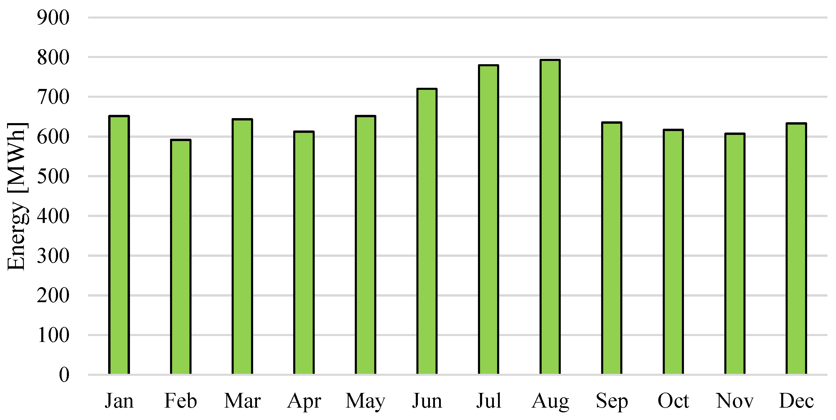
In terms of energy demand variability on the annual scale, Figure 2 shows that the highest energy demand is observed in summer months (which in the northern hemisphere are from June to September). In June, July and August the energy demand is above the mean by 8.8%, 17.9% and 19.8% on average, respectively. The lowest energy demand can be observed in February and April, and is below the mean by 11% and 8%, respectively.

Meanwhile, on a monthly scale, the variability of demand can to some extent depend on month length (February) and number of holidays, but is most closely related to the impact of air temperature on power demand (this issue will be discussed in detail in Section 3.3).

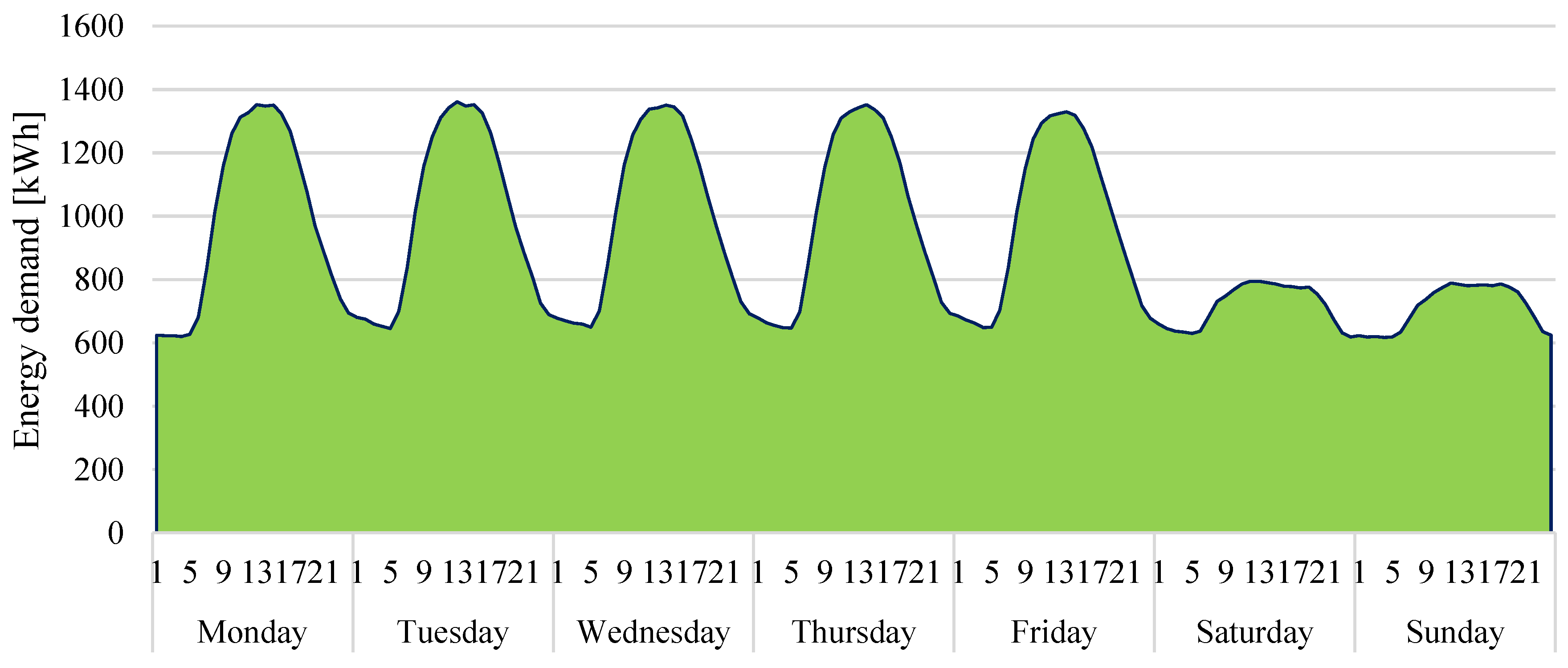
On a weekly time scale, the energy demand starts to exhibit clear and repeatable patterns, shaped mainly by the typical office building work hours. Figure 3 shows this pattern, with a clear reduction in energy demand during non-working hours from 1900 to 0600 and days off (Saturday and Sunday). Please also note the small drop in energy demand around midday (visible here from Monday to Wednesday), which may be related to the lunch break. For an office building there is also a notably high daily variability in energy demand. Based on this weekly energy demand pattern (averaged values over three years) it can be said that the so-called “baseload” is on average 615 kWh, whereas the peak demand can be over twice that and amount to 1361 kWh. The three-year hourly time series shows, however, that the minimal observed energy demand was 381 kWh and the maximal can be 6.5 times higher (2487 kWh).

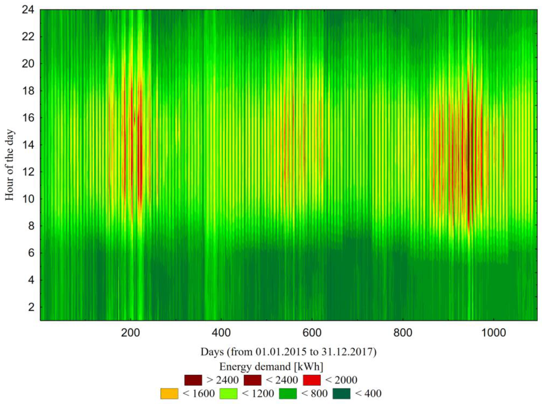
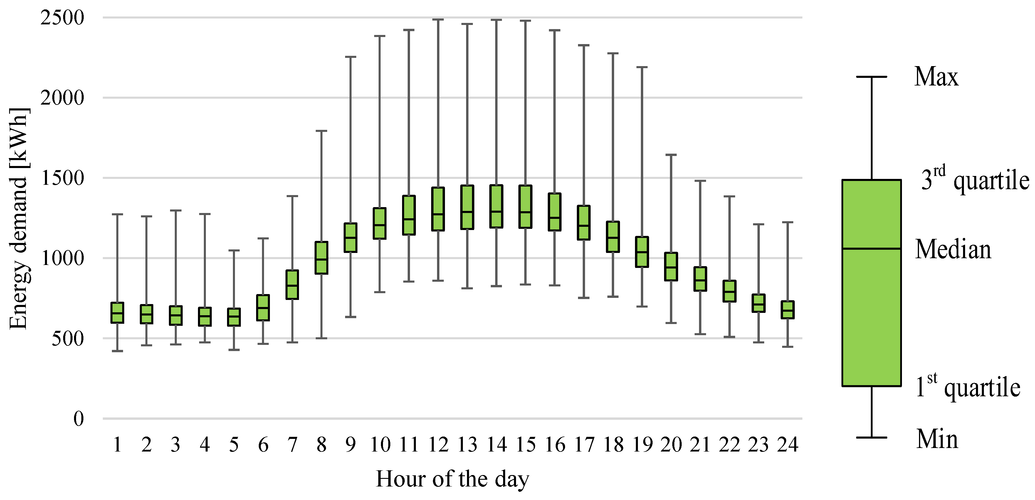
The final part of the energy demand analysis focuses on the daily pattern. This is presented in Figure 4 in the form of a box plot. Here only working days are considered. The box plot presents minimal and maximal values, as well as the median and the range of the 1st and 3rd quartile. As can be seen, the observed energy demand during working days ranges from 440 kWh to 2487 kWh. The highest energy consumption is observed during normal building operating hours from 0800 to 1900. On average, during those hours the office building consumes over 62% of its daily energy demand.

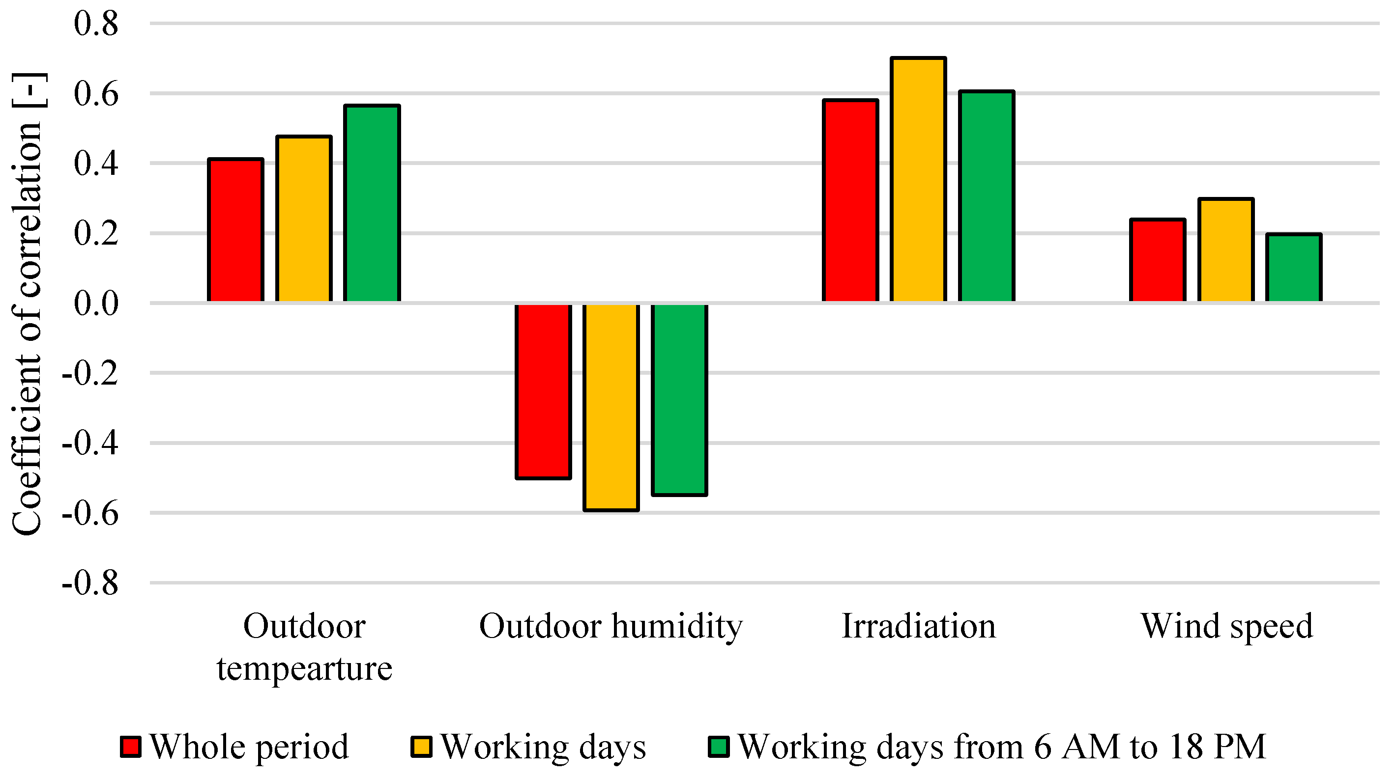
3.3. Correlation with Meteorological Parameters

As the building’s indoor environment is influenced by a multitude of factors (number of tenants, type of activity, heat output of appliances, the building’s thermal inertia and weather conditions) it often has to be shaped artificially by using various heating, ventilating and air-conditioning appliances (HVAC) that require electricity. Therefore, the second part of the analysis focuses on calculating correlation coefficients between observed energy demand and the four selected (available) meteorological parameters (temperature, humidity, irradiation and wind speed). As the office building exhibits some typical weekly and daily energy demand patterns, we divided the available data into three sets: the whole period (all available data); working days (from Monday to Friday and excluding holidays); and working days as in the second subset, but limited to the working hours of 0600 to 1800.

The coefficients of correlation are presented in Figure 5. In general, a positive linear correlation was observed for temperature, irradiation and wind speed, whereas there was a negative correlation for humidity. The correlation between energy demand and wind speed was relatively low and the highest value was close to 0.3 for the subset that considered only working days. In the case of temperature, the highest value (0.56) was for working days but considering only working hours. For the two remaining parameters the highest values were observed for whole working days and were -0.59 for humidity and 0.70 for irradiation.

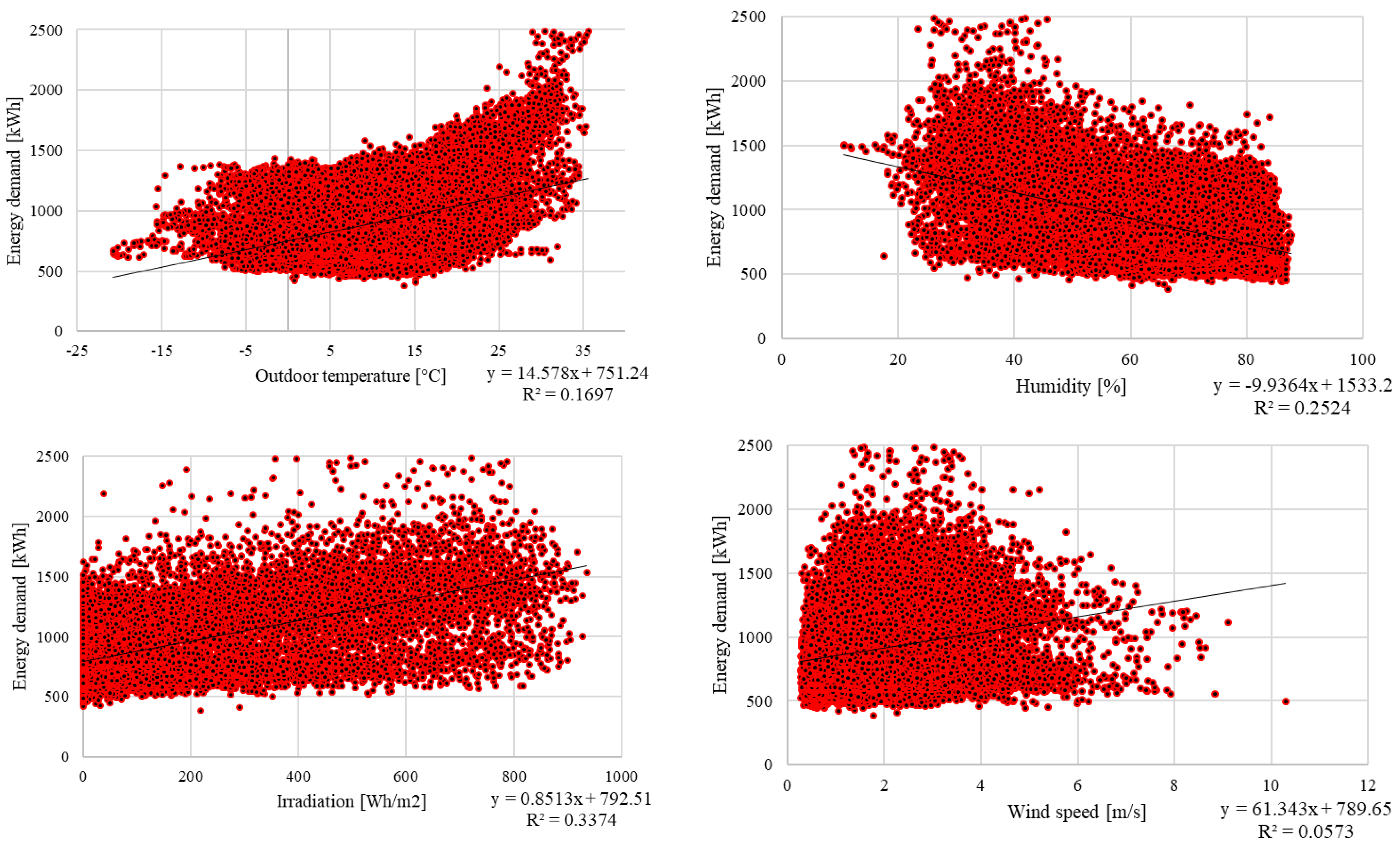
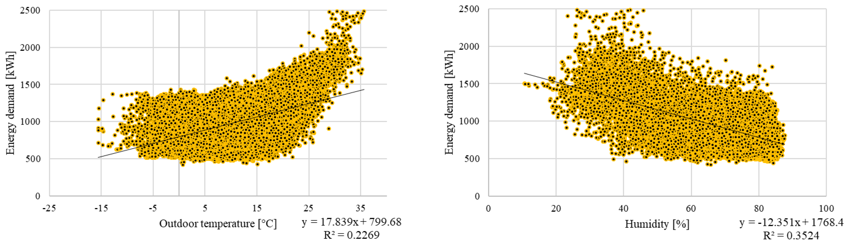
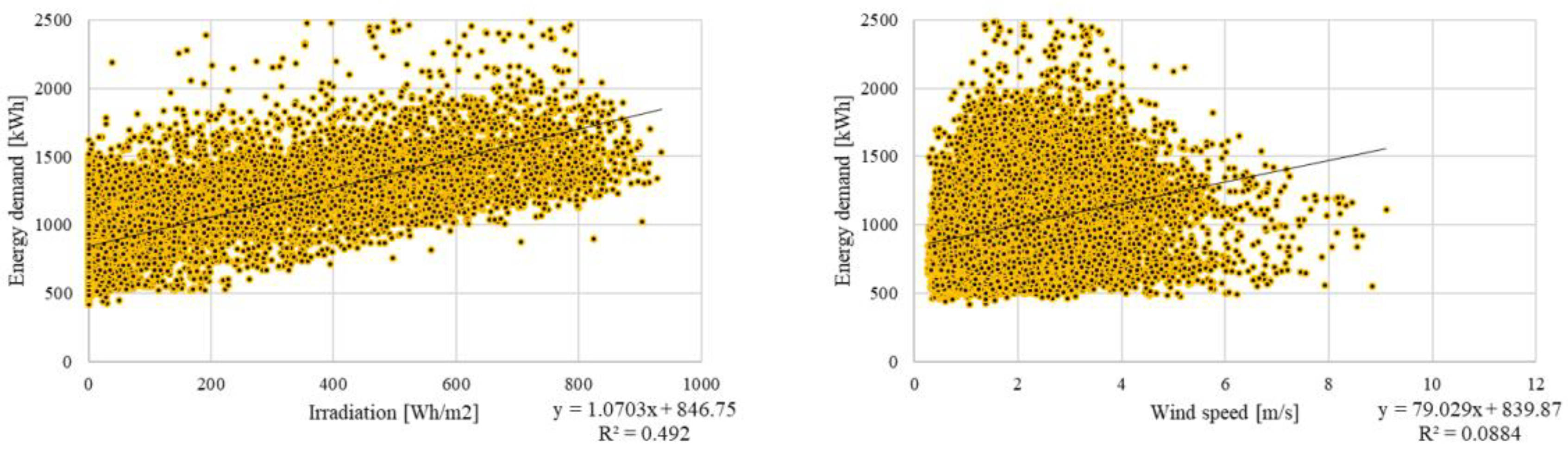
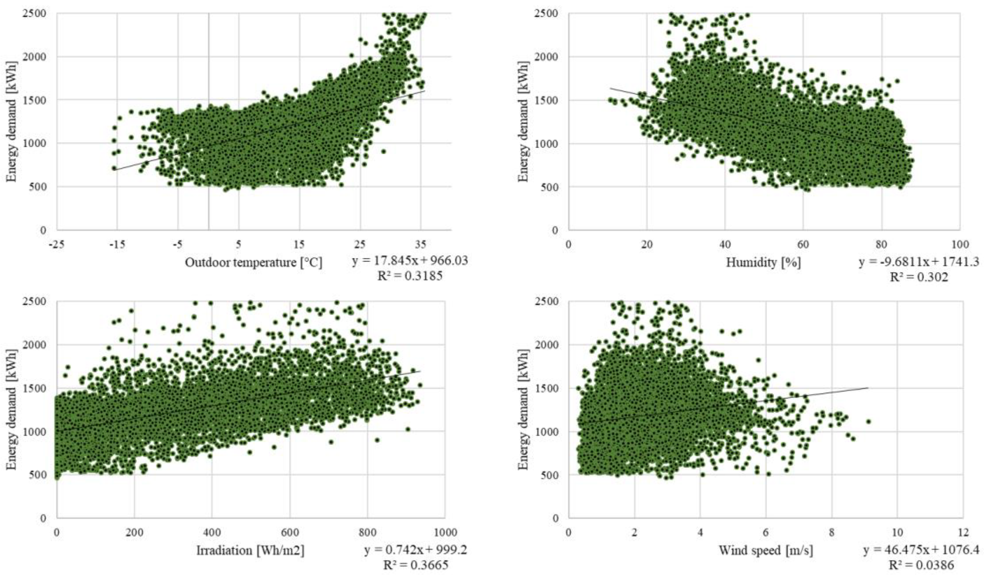
Figure 6 and Figure 7 present the relationship between meteorological parameters and energy demand as scatter plots. As can be observed, an interesting relationship emerges between energy demand and irradiation and temperature. Namely, after exceeding a certain temperature threshold the energy demand starts to increase very rapidly (Figure 7, Figure 8 and Figure 9, charts–upper left corner). This results from the fact that the high outside air temperature requires the cooling processes inside the building to be intensified to maintain the required thermal comfort. In general, it can also be noted that there is a greater energy demand when humidity is low (especially lower than 50%) and energy demand tends to increase with increasing irradiation. However, for each scatter plot for which a linear trend line has been added, the coefficient of determination is lower than 0.5, which indicates that the fit is relatively low and this meteorological parameter does not satisfactorily reflect energy demand.

3.4. Cluster Analysis—Energy Demand and Meteorological Parameters

The last part of this study on energy demand patterns is a cluster analysis which aims to distinguish typical daily energy demand and meteorological parameter patterns. Only three meteorological parameters (irradiation, humidity and temperature) were considered, because they exhibited the highest absolute correlation coefficients with energy demand. The available data is rearranged in such a manner that each day is described by 96 values (24 for each meteorological parameter and energy demand) with a total number of 1096 cases/days. The clustering was performed in Statistica version 12 software from StatSoft (Dell) by means of a k-clustering algorithm with an objective to maximize the Euclidian distance between the centers of the major clusters whilst minimizing the distance between the cases assigned to those clusters. The algorithm was run on a personal computer equipped with 16 GB of RAM and Intel® Core™ i7-7740X CPU with eight cores each rated at 4.3 GHz. Prior to applying the k-clustering algorithm the data was normalized to the 0–1 range to ensure its equal importance in creating the clusters. The results of the analysis are presented in Figure 9, Figure 10 and Figure 11. As can be observed, it was possible to distinguish three clusters of typical days from the perspective of energy demand and meteorological parameters. The days assigned to the cluster presented in Figure 9 constitute 48.2% of considered cases, and those in Figure 10 and Figure 11 constitute 24.5% and 27.3%, respectively.

For better description and understanding of the charts presented in Figure 9, Figure 10 and Figure 11 the statistical parameters (average and sum) of those values are aggregated in

Table 1. Short summary of the three clusters and their parameters.

Cluster	Sum of Energy Demand (MWh)	Sum of Irradiation (kWh/m2)	Average Outdoor Temperature (°C)	Average Outdoor Humidity (%)
A	20.389	1.206	4.549	70.581
B	25.318	6.384	19.856	52.191
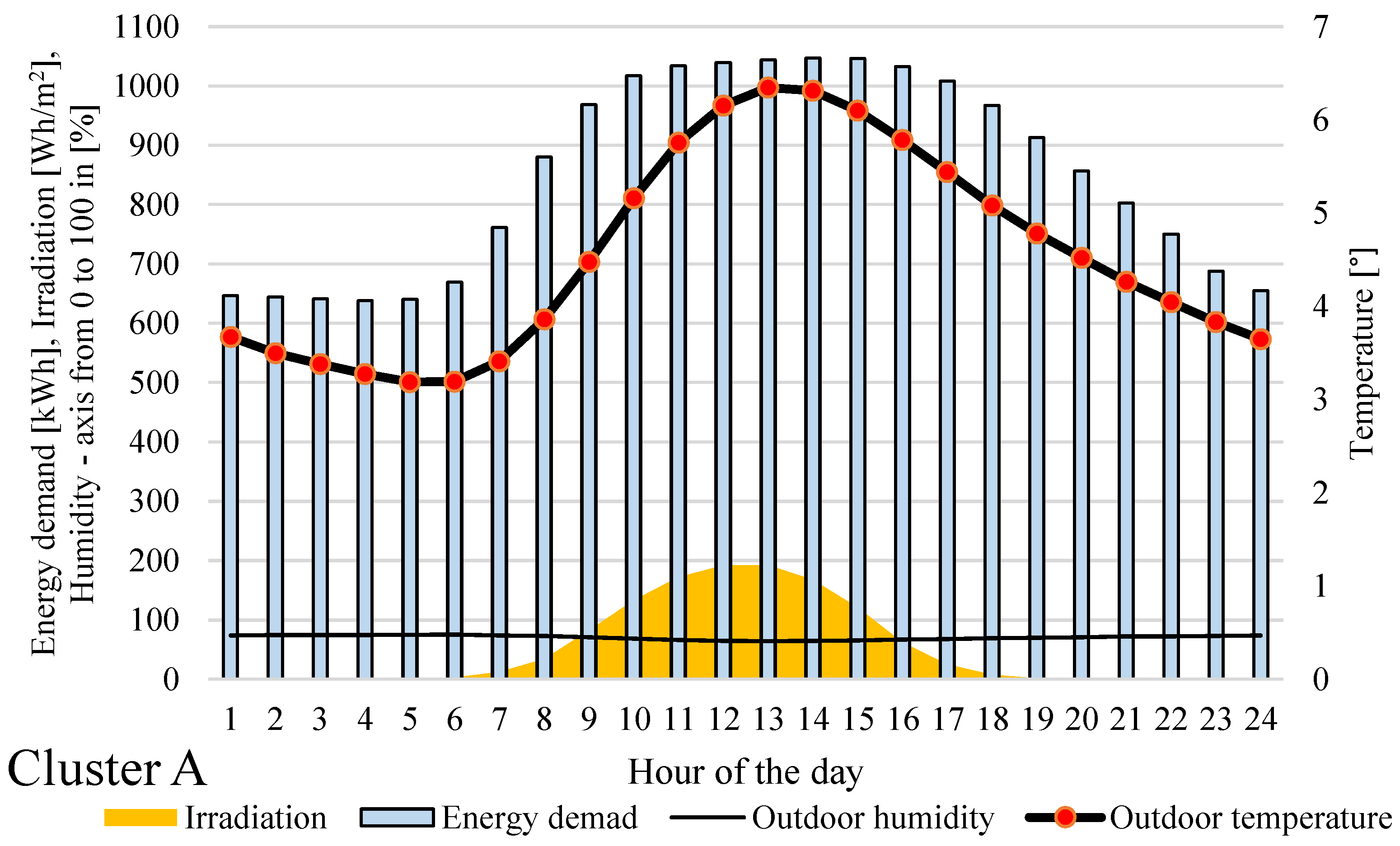
C	20.833	3.748	12.763	60.143

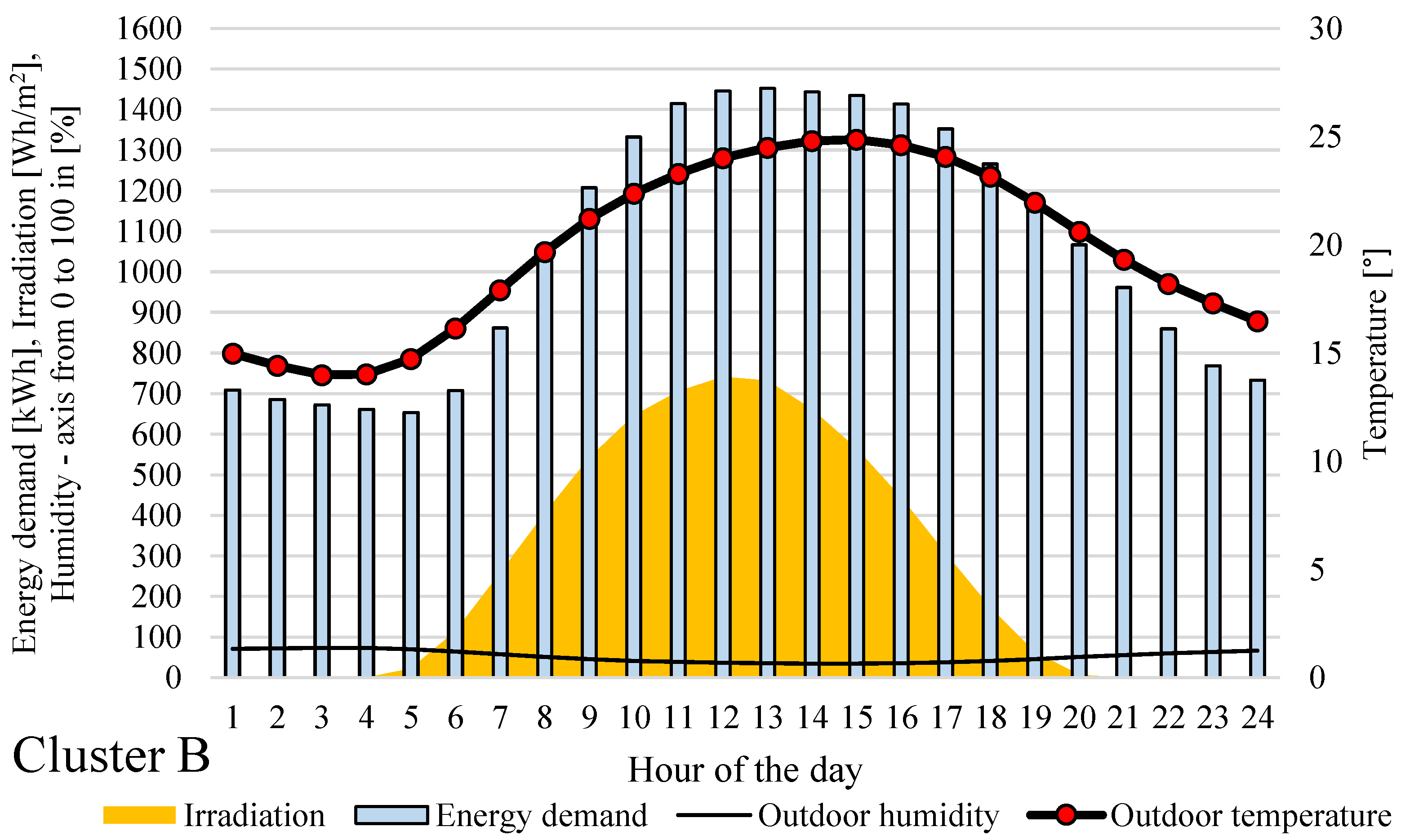
. As can be seen, cluster A (Figure 9) is a typical, rather cold day (average temperature below 5 °C) with a low daily sum of irradiation, and simultaneously the lowest observed energy demand of the three cases. 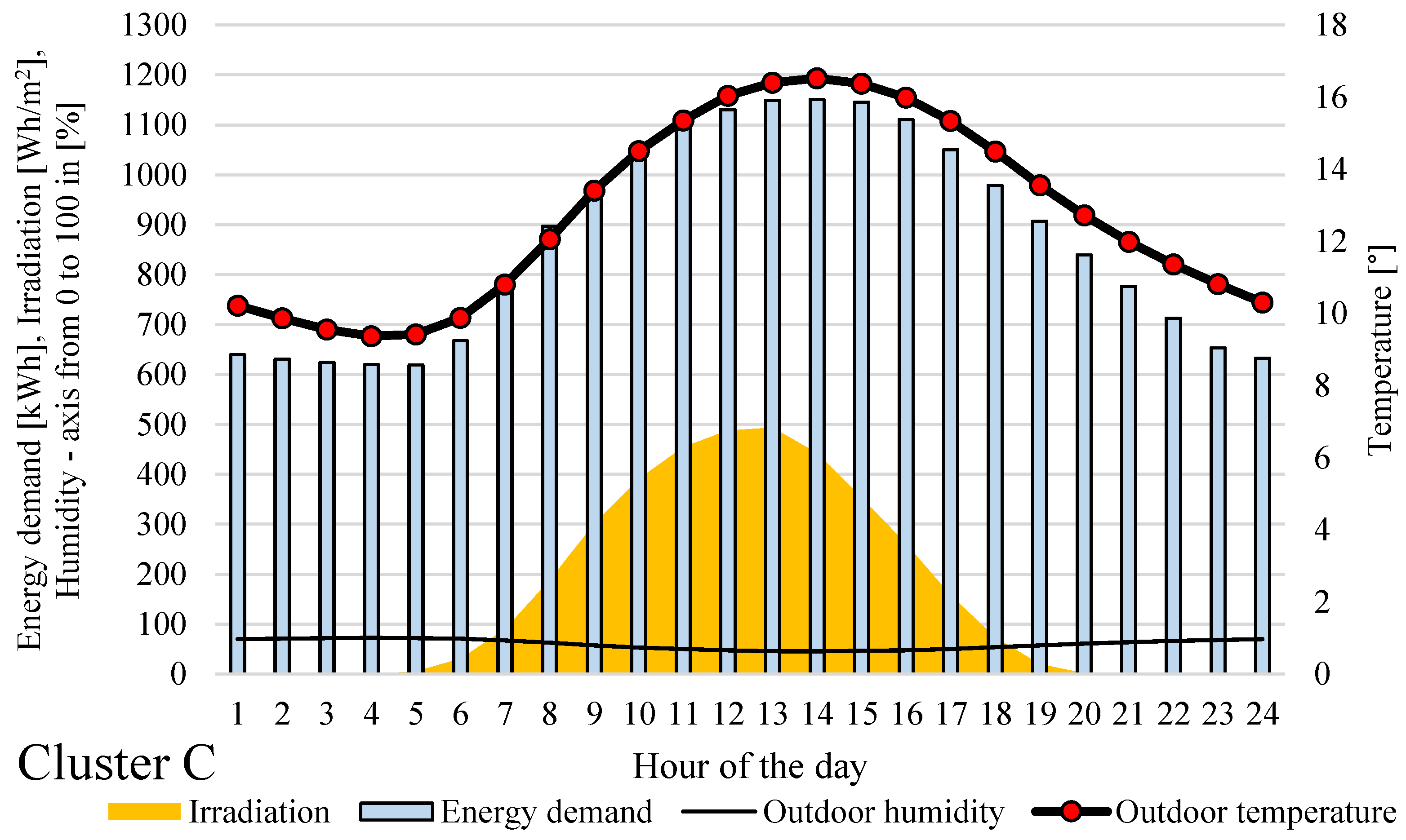Cluster B (Figure 10) represents a relatively warm day (average temperature close to 20 °C) with relatively low humidity (slightly above 50%) and a high daily sum of irradiation (above 6 kWh/m²); at the same time, this cluster is characterized by the highest energy demand (25.3 MWh). In contrast, cluster C (Figure 11) is an intermediary between clusters A and B, and has a slightly higher energy demand than cluster A (by 0.5 MWh) but at the same time is characterized by a daily sum of irradiation that is over three times greater and an average daily temperature that is over eight degrees higher. A combination of Table 1 and Figure 9, Figure 10 and Figure 11 very clearly shows the relationship between meteorological parameters and energy demand. It is especially visible in the case of temperature and energy demand in Figure 9, Figure 10 and Figure 11, where the column plots and dotted line seem to follow the same pattern.

3.5. Modelling Power Demand—Regression Analysis

In this section a multiple linear regression (MLR) analysis was performed to find out how well the power demand can be modeled based on meteorological parameters such as wind speed, temperature, humidity and irradiation. Since all of these parameters are statistically significant at p < 0.05, all were included in the MLR analysis. The MLR was used to identify the strength of the effect that the independent variables (meteorological parameters) have on the dependent variable (power demand). All necessary calculations were performed in MS Excel and its inbuilt toolbox designed for statistical analysis. In total, three MLR models (Equations (1)–(3)) have been constructed covering: whole period–M1, only working days–M2 and working days from 0600 to 1800–M3, respectively.

The following equations present the results of the regression analysis:

$$P_i^{*}=4.31T_i-3.31h_i+0.56H_i+18.54v_i+959.36$$

(1)

$$P_i^{*}=4.19T_i-3.38h_i+0.75H_i+21.55v_i+1043.67$$

(2)

$$P_i^{*}=7.99T_i-2.89h_i+0.37H_i+14.71v_i+1126.79$$

(3)

where: $P_i^{*}$ is modeled power demand in hour i (kW), $T_i$ is temperature in hour i (°C), $h_i$ is humidity in hour i (%), $H_i$ is irradiation in hour i (Wh/m²), and $v_i$ is wind speed in hour i (m/s).

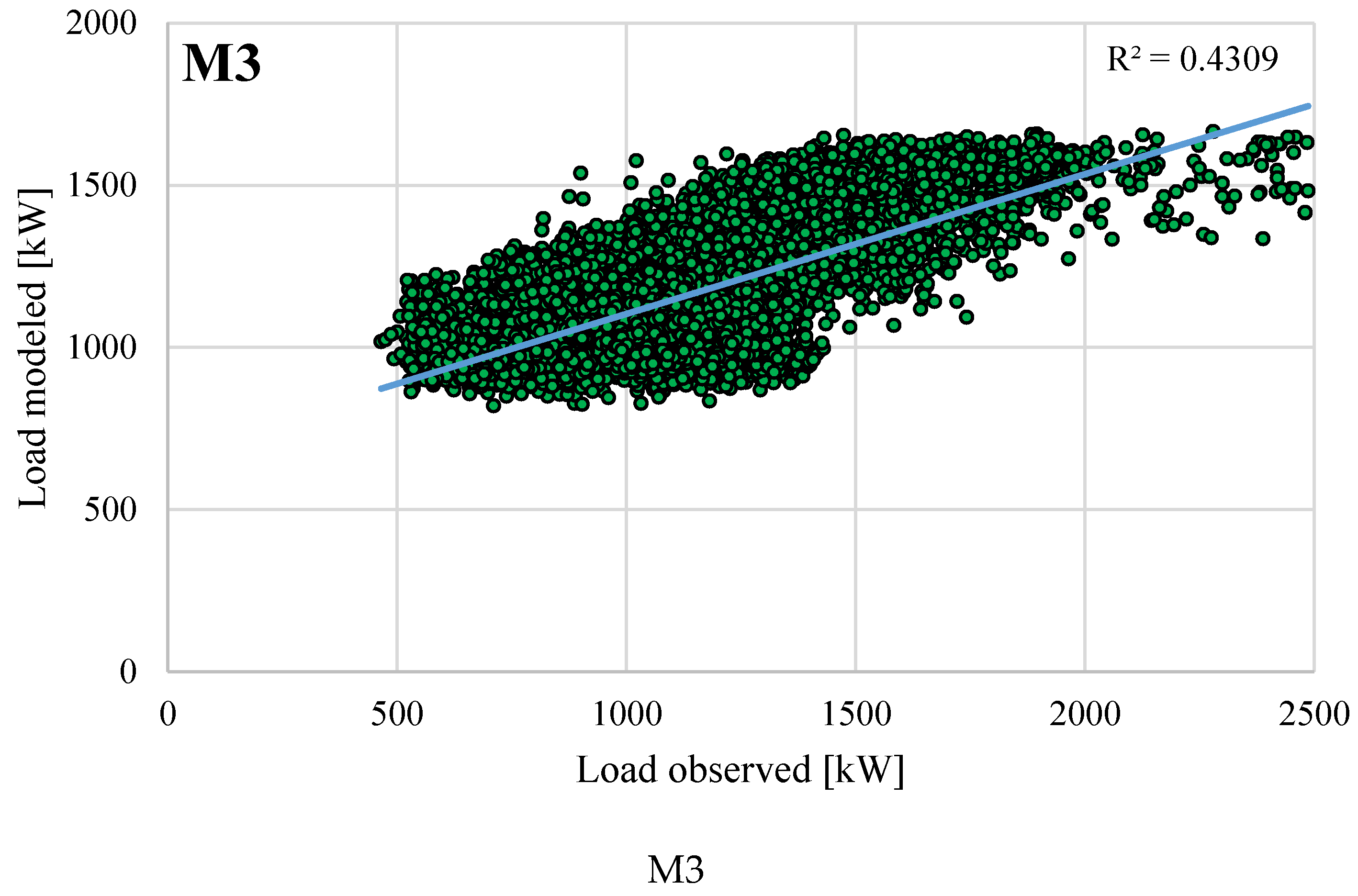
In Figure 12, scatter plots for all the considered models have been presented. As can be observed, the models exhibit relatively low values of the coefficient of determination (R²) which ranges from 0.37 for M1, through 0.43 for M3 and 0.53 for M2, indicating that based on the available independent variables the model can explain up to 53% of the variability in the response data (dependent variable) around its mean. What is also visible from the charts presented in Figure 12 is that the models were not capable of accurately modeling the highest values of the power demand.

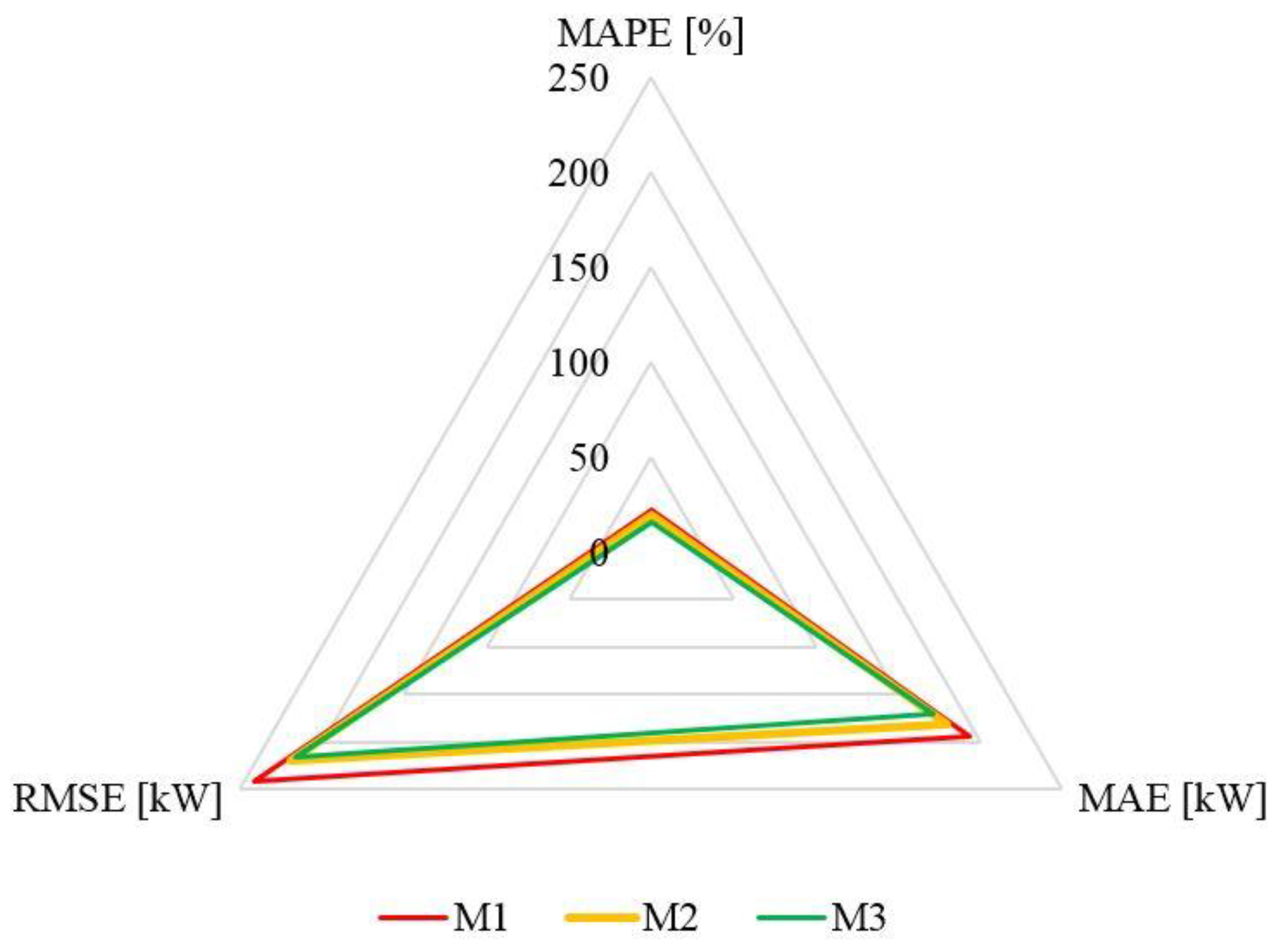
For a more detailed analysis of the regression models’ performance they were further assessed based on the following statistical criteria: mean absolute percentage error (MAPE), mean absolute error (MAE), and root mean squared error (RMSE) calculated as in Equations (4)–(6).

$$MAPE=\frac{1}{n}{\displaystyle \sum }_{i=1}^n\left|\frac{P_i-P_i^{*}}{P_i}\right|$$

(4)

$$MAE=\frac{1}{n}{\displaystyle \sum }_{i=1}^n\left|P_i-P_i^{*}\right|$$

(5)

$$RMSE=\sqrt{\frac{1}{n}{\displaystyle \sum }_{i=1}^n{\left(P_i-P_i^{*}\right)}^2}$$

(6)

where: $P_i^{*}$ is modeled power demand in hour i (kW), P_i is actual power demand in hour i (kW), P_i and $P_i^{*}$– are according to the arrangements for patterns (1), (2) and (3).

In terms of the considered three models assessment criteria (Figure 13), the M3 model which was applied for working days from 0600to 1800 showed the lowest values. This indicates that it outperformed the two remaining models in its ability to more accurately model the power demand. The mean absolute percentage error (MAPE) of the M3 model was equal to 16.3% whereas for M1 it was 22.5%. The reduction in modeling errors (or in other words, an increase in modeling accuracy) was achieved due to limiting the time frame that the model has to cover (from the whole period to only working days from 0600 to 1800).

It must be highlighted that using MRL assumes that a linear relation exists between dependent and independent variables. Therefore, if temperature-load or another pair of variables exhibit a different non-linear relationship, better accuracy may be achieved if tools like artificial neural networks were applied. In general, the quality of the MLR models shows that some remaining factors/variables, which also have a significant impact on the power demand but were not considered in this analysis.

4. Discussion

It is well-known fact that meteorological parameters influence the electricity demand in office buildings. Additional energy is required to maintain an adequate working environment by, for example, removing excessive heat (cooling). The rich literature available on the relationship between meteorological parameters and load is missing evidence from an office building located in Central Europe, including Poland. The selected building was awarded a gold certificate accordingly to LEED standards which makes it representative for its class. The conducted research is of importance, and most importantly it is in line with the EU goals, which aim at reducing the human impact on the natural environment. Although the presented results are preliminary, the paper gives insight into the volatility of electricity demand in an office building located in Poland. The outcome of the conducted analysis can be used as an input or premise in office building modeling for various climate change scenarios, building participation in demand side management, and deployment of photovoltaic installations.

This study measured the relationship between the meteorological parameters and electricity demand as well as aimed at distinguishing typical load patterns based on well-known statistical tools including the Pearson coefficient of correlation, k-clustering method and multiple linear regression analysis. This approach enabled us to confirm the correlation between load and meteorological parameters as well as to single out daily and weekly demand patterns. Unfortunately, the outcome of this study is limited by the nature of the applied tools, such as the inability of the Pearson coefficient of correlation to grasp the non-linear dependencies between variables or the assumption of multiple linear regression that independent and dependent variables are in a linear relationship. Additionally, this research (a case study) covered only one building; therefore, it is mandatory to conduct a further analysis on a larger sample to draw more generalizable conclusions. What is more, the results of the correlation analysis indicating that meteorological parameters’ correlation values with load, make them suitable input variables for load forecasting models. Meaning that, in the case of an office building the load can be forecasted based on commonly available day ahead hourly weather forecasts (which is an interesting research direction).

As the results have shown that an increasing outdoor temperature leads to greater energy demand, the facility manager can undertake preventive actions to reduce the energy consumption. The manager’s activities can be based on available weather forecasts and concentrate on adjusting the indoor environment to meet the next day’s predicted changes. For example, building thermal inertia can be used to maintain the required air temperature for the next day by cooling or heating the building overnight (when energy is usually cheaper). The observed energy demand patterns show that the highest energy demand is around (working day) midday when the irradiation values are also reaching their maximum. This means that office buildings are suitable for the deployment of photovoltaic installations, which reduce the building environmental impact. However, the analysis also shows that the installation must be properly sized as the energy demand over the weekend is relatively low (without a distinguishable peak) and oversized photovoltaic installation may generate significant energy surpluses (which can be either stored or sold to the grid–depending on the applied solution).

The cost of running the analysis performed in this study depends on the software availability. The correlation study can be performed in commonly used MS Excel or its freeware version (OpenOffice). The clustering analysis requires more sophisticated software although k-clustering algorithm applications are available in MS Excel using its inbuilt programming language VBA. Considering the above, the costs of similar analysis can be significantly reduced. However, it is harder to estimate the potential benefits of such analysis. Pure knowledge of the relationship between several variables or the demand patterns does not directly lead to energy savings or other forms of benefit. The conducted analysis does not provide ready to use solutions and should be treated as a preliminary study of factors influencing the energy demand in office buildings located in Central Europe. Therefore, the outcome of this paper may be used as a premise for a further analysis, which will aim, for example, at forecasting the office building load.

The applied methodology was based on well-known and established statistical methods/tools. Therefore, this approach can be used in the case of other buildings. However, the results are most likely only representative for a building that was awarded a golden LEED certificate. What is more, the energy demand can be influenced by other factors which were not taken into the consideration and does not depend on construction materials used to create the building. For example, electricity load may also be driven by the fact that that some tenants perform their activities overnight due to time differences between this site and company headquarters (what may disturb the results of this analysis).

Knowing how meteorological parameters shape/influence the energy demand in office buildings also provides important feedback for decision makers on a regional and national level. The known and planned spatial distribution of office buildings within a city gives information about potential requirements with regard to the infrastructure development. Also, having projections for the future number of office buildings and their typical load profiles provides significant information about how (depending also on meteorological parameters) they might influence the local and nationwide load demand. This knowledge may provide significant benefits in future distribution network development. Also, awareness of the typical load patterns in an office building may incline decision makers to devise suitable incentives that support the development of photovoltaic installations.

Finally, it should be noted that the results presented in this study are part of a research project aimed at analyzing the potential that office buildings have to participate in the energy market as virtual power plants. Therefore, future research will focus on creating office building energy demand forecasting models especially tailored to Polish climatic conditions, and on applying them to existing office buildings. The next steps will also consider the role of photovoltaics in increasing office buildings’ energetic self-sufficiency and minimizing their impact on energy demand.

5. Conclusions

This research aimed to analyze the energy consumption of an office building in southern Poland (Kraków). As input data, three-year time series of hourly energy demand, temperature, irradiation, humidity and wind speed were used. Such analysis was required as a literature gap was identified with regard to office buildings located in Central Europe (Poland) and their typical energy demand patterns. An office building awarded with a golden LEED certificate was selected as a case study, which makes the results representative for this class of buildings.

The conducted analysis revealed not only that the office building’s load profile exhibits significant and repeatable daily and weekly load profiles, but also that energy demand is positively correlated with meteorological parameters. The presence of distinguishable energy demand patterns makes this research a valuable contribution for decision makers and planners as it provides information about the office buildings’ impact on the regional and also nationwide energy demand. The demand patterns also highlight the potential for the deployment of photovoltaic installations, although not without some additional analysis (as over the weekend the energy demand is significantly lower) because the energy produced by photovoltaics may not be consumed on site.

The final part of the research focused on a clustering analysis, which revealed that it is possible to distinguish three typical daily energy demand patterns and their associated meteorological parameters. The established clusters can be further used in hybrid forecasting models.