Impacts of Freight Transport on PM_2.5 Concentrations in China: A Spatial Dynamic Panel Analysis

Abstract

Freight transport policies have been developed to reduce air pollution in China. This paper aims to evaluate the impact of a freight modal shift on PM_2.5 concentrations using the panel data of 30 provinces in China over the period 1999–2016. The direct and spillover effects of a freight modal shift on PM_2.5 concentrations in China, as well as the effects of other socioeconomic factors, were estimated by employing spatial dynamic panel data models. In particular, the channel through which the freight modal shift might be beneficial in reducing PM_2.5 concentrations was examined. The results show that PM_2.5 concentrations in China do not only decrease with a modal shift of freight from road to rail in a province, but also and to a larger extent with that in neighboring provinces. However, there exist heterogeneous effects across different regions of China. The interaction between a freight modal shift and energy efficiency may lead to a decrease in the PM_2.5 concentrations, but only in the central and western regions. These findings provide suggestions for government policies directed to sustainable development.

1. Introduction

Air pollution, especially fine particulate air pollution, has become one of the major environmental issues in China. The extremely severe haze events that occurred in the first quarter of 2013 affected about 13.5% of the land area and 800 million people in China [1]. The particulate matter pollution threatens air quality, climates and human health. Fine particulate matter, which can easily enter the lungs and even the blood, is responsible for adverse health effects, including an increased risk of premature mortality and higher rate of adverse respiratory health indicators [2]. The adverse effect of particulate matter pollution causes substantial economic losses. It is estimated that without a pollution control policy, the particulate matter pollution in China will lead to a 2% GDP loss and 25.2 billion USD in health expenditure in 2030 [3]. A number of plans and policies have been implemented to deal with the air pollution. China’s State Council released the “Air Pollution Prevention and Control Action Plan” in September 2013, which set several milestones for reducing PM_2.5 concentrations in the Beijing-Tianjin-Hebei region, Yangtze River Delta region, and Pearl River Delta region.

The transportation industry has experienced rapid growth in recent years and has contributed to industrialization and urbanization in China. According to China’s National Bureau of Statistics (NBS), the freight transport volume in China increased from 4.4 trillion ton-kilometers (tkm) in 2000 to 19.6 trillion tkm in 2017, with an annual growth rate of 9.2%. However, as shown in Figure 1, there were significant changes in the shares of the five freight transport modes in China (i.e., road, railway, waterway, aviation, and pipeline). In 1985, the shares in road, railway, waterway, aviation and pipeline were 14.6%, 62.34%, 18.41%, 0.03% and 4.63%, respectively. In 2017, these shares became 47.3%, 19.12%, 30.04%, 0.17% and 3.37%, respectively. Road freight transport has become the dominant freight transport mode. While the rapid development of freight transport contributed to China’s economic growth, the increase of road freight transport resulted in a higher energy consumption and air pollutant emissions. In particular, the fossil fuel consumption in the road transport sector contributed to the particulate matter pollution. A latest source apportionment analysis of the PM_2.5 concentrations in China’s 15 cities indicated that the proportion of mobile sources (e.g., vehicles) ranged from 13.5% to 52.1% in 2017. Motor vehicle emission has been one of the major PM_2.5 sources [1]. Buses, taxis and inter-city coaches are responsible for traffic-related particulate matter emissions, although the major contributor is road freight transport [4].

For sustainable economic development in China, it is necessary to develop an environmentally friendly transport system. Particulate pollutant mitigation, especially in the transportation industry, is becoming the most important agenda in China. However, a prerequisite for effective mitigation strategies is the identification of the factors contributing to particulate matter pollution. Many existing studies have focused on the identification of the chemical composition and characteristics of PM_2.5 [1,5,6]. A growing number of studies investigated the relationship between socioeconomic factors and environmental pollution [7,8,9,10,11]. Industrialization, urbanization, energy consumption and vehicle population are identified as major socioeconomic factors contributing to China’s particulate matter pollution [12,13,14]. Decomposition analysis, including index decomposition analysis (IDA) [15] and structural decomposition analysis (SDA) [16], were employed to identify the socioeconomic factors driving particulate pollution. Guan et al. [17] measured the magnitudes of different socioeconomic factors in driving the primary PM_2.5 emission in China between 1997–2010 using a structural decomposition analysis. PM_2.5 concentrations in one unit exhibit a positive relationship with PM_2.5 concentrations in its neighboring units [18]. Therefore, spatial correlations in the particulate matter pollution of geographically nearby units should be considered to avoid biased and inconsistent estimations. Spatial econometric models considering the spatial interactions among geographical units were used to analyze the impacts of socioeconomic factors on air pollutant emissions [19,20,21]. Fang et al. [22] quantitatively estimated the impacts and spatial variations of urbanization on China’s air quality by employing the spatial lag model (SLM) and the geographically weighted regression. The spatial lag model and spatial error model (SEM) were utilized by Hao and Liu [23] to investigate the impacts of socioeconomic development indicators, such as GDP per capita, industry and transport, on PM_2.5 concentrations in China.

The modal shift of freight transport to rail provides a logical solution for air pollution, originating from long-distance freight transport [4]. Previous studies have estimated the economic and environmental costs of different freight transport modes [24,25], although the spatial impacts of a freight modal shift on air pollution, especially on particulate matter pollution, have been paid less attention. Since 2017, China has intensified the efforts to increase the share of rail freight transport, as part of the strategy to reduce particulate matter pollution. “Transportation Structure Adjustments Three Years Action Plan” was proposed in 2018 to promote a road-to-rail freight modal shift and reduce air pollution. In the action plan, China expects to cut its emission of fine particulate matter by 55,000 tons through transportation structure adjustments over three years. More specifically, from 2018 to 2020 China aims to increase its rail freight volume and waterway freight volume by 1.1 billion tons and 500 million tons, respectively, and to reduce the road freight volume linked to coastal ports by 440 million tons. However, the effectiveness of a road-to-rail freight modal shift remains unknown. This paper aims to empirically investigate the spatial effects of socioeconomic factors, in particular a freight modal shift, on particulate matter pollution, and to provide suggestions for freight transport policies. The spatial dependence and heterogeneity of PM_2.5 concentrations in China were examined by employing spatial dynamic panel data models. More specifically, we estimated the direct and spillover effects of a road-to-rail freight modal shift on PM_2.5 concentrations in China and examined whether the shift of freight might interact with energy efficiency and thus affect particulate matter pollution. The heterogeneity in the interaction effects between a modal shift of freight transport and energy efficiency across different regions of China was examined as well.

The remainder of this paper is organized as follows. Section 2 describes the variables and data used in our study; Section 3 presents the spatial dynamic panel data model employed in the empirical analysis; Section 4 discusses the results of the spatial econometric analysis and robustness checks; Section 5 provides some concluding remarks.

2. Variables and Data

For the indicator of particulate matter air pollution, the log of the annual average concentration of PM_2.5 (LPM) was used. PM_2.5 data were extracted from the global PM_2.5 grids (1998–2016) using the ArcGIS. The PM_2.5 grids, provided by the Battelle Memorial Institute and the Center for International Earth Science Information Network (CIESIN) at Columbia University, consist of annual concentrations (micrograms per cubic meter) of ground-level fine particulate matter (PM_2.5) per 0.01 degree grid cells. The GEOS-Chen chemical transport model was used to relate the total column measure of aerosol, obtained from NASA’s Moderate Resolution Imaging Spectroradiometer (MODIS), Multi-angle Imaging SpectroRadiometer (MISR), and the Sea-Viewing Wide Field-of-View Sensor (SeaWiFS), to near-surface PM_2.5 concentrations [26]. China’s PM_2.5 concentrations for 1999 and 2016 are shown in Figure 2.

Three categories of socioeconomic factors were considered: Transportation, economic development and energy consumption [1,13,23]. The transportation factors include a freight modal shift and road congestion. The road freight transport of vehicles, in particular diesel freight trucks, accounts for a large portion of PM_2.5 concentrations. Rail freight pollutes the air as well, but its contribution is much lower [24]. The ratio of rail freight volume to road freight volume (RFV) was used as an explanatory variable to evaluate the environmental benefits of a road-to-rail freight modal shift [27]. Road congestion was also considered. In 2017, the number of vehicles registered in China reached 310 million, with an annual growth of 5.1%, and private cars accounted for two-thirds of the vehicle population. The rapid growth of the vehicle population had brought about serious pollution problems. Previous studies showed that nitrogen oxides, organic hydrocarbons, black carbon, and many other pollutants generated from vehicular gas were the main components of urban PM_2.5 [28,29]. Since low speed driving and transient driving modes are more polluting than steady-speed driving [30], PM_2.5 concentrations near busy roads could be 30% higher [31]. Therefore, as another explanatory factor of transportation, road congestion, measured by the number of private cars per kilometer of road (NC), was used.

The economic factors considered in this study are economic growth and trade openness. The Environmental Kuznets Curve (EKC) hypothesis provides a theoretical basis for the relationship between GDP per capita and the environment [32]. According to the theory, the positive relationship between economic growth and environment pollution is reversed when a peak level of emissions is reached. However, empirical studies showed that the shape of the EKC curve depended on the type of pollutants [33]. In our study, the log of real GDP per capita (LGDP) was used to account for the influence of economic development on PM_2.5 concentrations. Meanwhile, previous studies showed that trade openness contributed substantially to air pollution [34,35]. Guan et al. [17] demonstrated that export was responsible for 10% of China’s primary PM_2.5 emissions. However, the influence of trade on air pollution is obscure in theory. The Pollution Haven Hypothesis (PHH) provides a theoretical explanation for the positive relationship between trade openness and air pollution. In Grossman and Krueger [36], however, the relationship between trade openness and environment was more complicated. According to the techniques effect, one of the three independent effects proposed in their study, liberalized trade might bring about environmentally beneficial production techniques and reduce air pollution. In our study, trade openness was measured as the share of trade (exports plus imports) in GDP (STG). To test the robustness of our analysis, we employed urbanization and industrialization as two additional variables. The former was measured by the share of urban population (SUP), while the latter was measured by the share of secondary industry in GDP (SSG).

Energy consumption, especially fossil fuel consumption, is a major source of fine particulate matter in China [6,37,38]. As main energy sources leading to particulate matter pollution, coal combustion and transport fuels contributed to 25% and 4% of the total primary PM_2.5 emissions in China in 2010, respectively [17]. Implementing energy efficiency measures in the industrial production process, especially in the iron and steel industry, would reduce greenhouse gas emissions and air pollutants in China [39]. Improving energy efficiency offers an excellent opportunity to mitigate transport air pollutants as well. Using alternative transport fuels for vehicles, especially for diesel freight trucks, would increase energy efficiency and improve air quality. Moreover, it is possible to improve the energy efficiency of freight transport by shifting from less efficient road freight to more efficient rail freight [40]. In this study, energy efficiency, measured as the ratio of real GDP to energy consumption (RGE), was used.

To examine the heterogeneous impacts of the freight modal shift on PM_2.5 concentrations across China’s four economic zones, the panel data used in this study were divided into four subsamples. The four economic zones are the Bohai Rim region (BR), the Yangtze River Delta and Pearl River Delta region (YRD-PRD), the Central Plain region (CP) and the Western region (W). The adjacent neighbors of a province may not be in the subsample, but the spillover effects of their PM_2.5 emissions on the sampled provinces still exist. To deal with this issue, we controlled for the (log of the) average of the non-sampled adjacent neighbors’ PM_2.5 concentrations (LPMN). The sample consisted of 30 mainland provinces (excluding Tibet) and ran over the period 1999–2016, during which we gathered raw data on the explanatory variables from the China Statistical Yearbook and provincial statistical yearbooks. Descriptive statistics for the full sample and the four subsamples were calculated. The means and standard deviations of our major variables are presented in

Table 1. The means and standard deviations of the variables.

Variable	Acronym	Full Sample	BR	YRD-PRD	CP	W
The log of the annual average concentration of PM2.5	LPM	3.233 (0.633)	3.810 (0.332)	3.371 (0.491)	3.582 (0.293)	2.784 (0.581)
The ratio of rail freight volume to road freight volume	RFV	1.833 (0.836)	2.783 (2.127)	0.431 (0.407)	2.168 (5.318)	1.961 (1.576)
The ratio of real GDP to energy consumption	RGE	0.844 (0.388)	0.936 (0.447)	1.260 (0.235)	0.827 (0.308)	0.624 (0.266)
The number of private cars per kilometer of road	NC	2.318 (1.131)	3.442 (1.055)	2.908 (1.143)	1.935 (0.820)	1.791 (0.793)
The log of real GDP per capita	LGDP	0.542 (0.746)	1.035 (0.650)	1.012 (0.627)	0.277 (0.611)	0.259 (0.682)
The share of trade in GDP	STG	0.312 (0.390)	0.560 (0.461)	0.760 (0.435)	0.095 (0.035)	0.110 (0.058)
The share of urban population	SUP	0.478 (0.157)	0.592 (0.193)	0.553 (0.163)	0.411 (0.087)	0.431 (0.123)
The share of secondary industry in GDP	SSG	0.389 (0.083)	0.408 (0.107)	0.387 (0.109)	0.414 (0.062)	0.372 (0.062)

Note: Standard deviations are given in parentheses. The units of LPM, RGE, NC, and LGDP are μg/m³, ten thousands yuan/tce, No. of cars/km, and ten thousands yuan/person, respectively. Source: PM_2.5 grids were obtained from CIESIN at Columbia University (http://sedac.ciesin.columbia.edu/data/sets/); raw data on the explanatory variables were gathered from the China Statistical Yearbook and provincial statistical yearbooks.

.

3. Methodology

3.1. Moran’s I

As a step preceding a more advanced quantitative analysis, the detection of spatial autocorrelation is necessary. Global and local Moran’s I indices [41] were used to investigate the spatial autocorrelation of PM_2.5 concentrations. The Global Moran’s I is

$$I=\frac{N{\displaystyle {\sum }_{i=1}^N{\displaystyle {\sum }_{j=1}^N{w}_{ij}\left(y_i-\overline{y}\right)}}\left(y_j-\overline{y}\right)}{S{\displaystyle {\sum }_{i=1}^N{\left(y_i-\overline{y}\right)}^2}},$$

(1)

where y_i and y_j are the values of the observed variable at provinces i and j; w_ij is the element in the spatial weight matrix; and S is the sum of all the elements of the weight matrix. A positive spatial autocorrelation is represented by a value of the Global Moran’s I statistics that is greater than zero and, inversely, a negative autocorrelation corresponds to a value less than zero.

The local version of Moran’s I was utilized to detect the local patterns of spatial autocorrelation. The Local Moran’s I is

$$I_i=\frac{\left(y_i-\overline{y}\right)}{{\sigma }^2}{\displaystyle {\sum }_{j=1,j\ne i}^N\left[w_{ij}\left(y_j-\overline{y}\right)\right]},$$

(2)

where y_i is the value of the observed variable at province i; y_j is the value of the observed variable at all the other provinces; σ² is the variance of the variable y; and w_ij is the element in the spatial weight matrix. Spatial clusters and outliers of PM_2.5 concentrations are identified by significant positive local Moran’s I and negative local Moran’s I, respectively.

3.2. Spatial Dynamic Panel Model

The concentration of PM_2.5 in a province will be determined by the PM_2.5 concentrations in neighboring provinces, and probably other variables in these provinces. Spatial econometric models deal with these co-determinants in the PM_2.5 concentrations, the explanatory variables and/or the error term from neighboring provinces [42]. This study employed the dynamic spatial Durbin models (SDM), including the temporal and space-time lags of the dependent variable. The dynamic spatial Durbin model is as follows:

$$Y_t=\tau Y_{t-1}+\rho W{Y}_t+\eta W{Y}_{t-1}+X_t\beta +W{X}_t\theta +Z_t\gamma +\mu +{\xi }_t+u_t,$$

(3)

where Y_t is a N × 1 vector of the dependent, that is, the log of the PM_2.5 concentrations for every province in the sample during time period t (t = 1, …, T); X_t denotes the N × K matrix of the explanatory variables that will be spatially lagged; β is the associated vector of coefficients; Z_t denotes the N × M matrix of the explanatory variables that will not be spatially lagged; γ is the associated vector of coefficients; W is a N × N spatial weight matrix; and WY_t and WX_t denote the endogenous spatial lag and the exogenous spatial lags, respectively. The strength of these spatial lags are measured by the scalar ρ and the vector θ. Y_t−1 is the temporal lag of the dependent variable and WY_t−1 is the one-period lag in the spatially lagged dependent variable. The scalars τ and η measure the strength of internal and external habit persistence. Furthermore, μ is a vector of spatial specific effects, ξ_t (t = 1, …, T) denotes time-period specific effect, and u_t is a vector of error terms. Two different spatial weight matrices were constructed. The first one is a binary contiguity matrix (W_bin), where the elements of the matrix would be 1, in the case of two provinces in contact, or otherwise 0. The other one is an inverse-distance weight matrix (W_dis), where the elements of the matrix would be the inverse of the distance of two provinces. Both types of matrices were row normalized. Model specifications were statistically tested by the (robust) Lagrange Multiplier (LM) tests and the likelihood ratio (LR) tests.

Departing from the above dynamic spatial Durbin model, the long-term impacts on the dependent variable, if the kth explanatory variable changes, are given by the N × N matrix:

$$\left[\frac{\partial E\left(Y\right)}{\partial x_{1k}}\cdots \frac{\partial E\left(Y\right)}{\partial x_{Nk}}\right]={\left[\left(1-\tau \right)I-\left(\rho +\eta \right)W\right]}^{-1}\left[{\beta }_k{I}_N+{\theta }_{k}W\right]$$

(4)

The direct effect of a change to the kth explanatory variable is defined as the average diagonal element of the matrix and the indirect effect (or spillover effect) is the average row or column sum of the off-diagonal elements [43]. Furthermore, by setting τ = η = 0, we can get the short-term direct and indirect effects.

4. Results

The purpose of our paper is to examine the spatial dependence and spatial heterogeneity of PM_2.5 concentrations in China. In particular, we estimated the spatial effects of a freight modal shift and investigated the channel through which a road-to-rail freight modal shift may be beneficial for the environment. More specifically, we examined whether the freight modal shift might interact with energy efficiency and thus affect PM_2.5 concentrations.

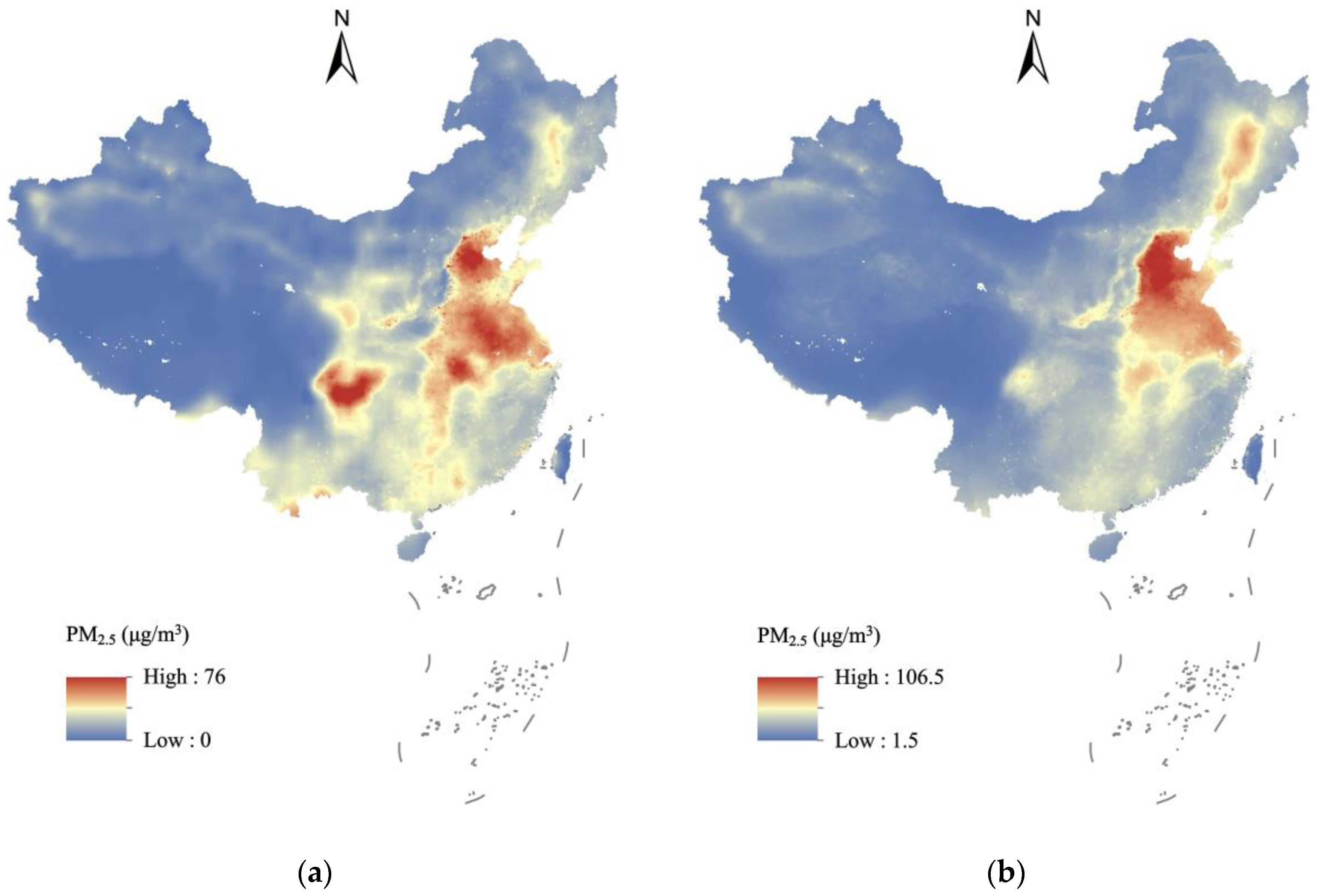
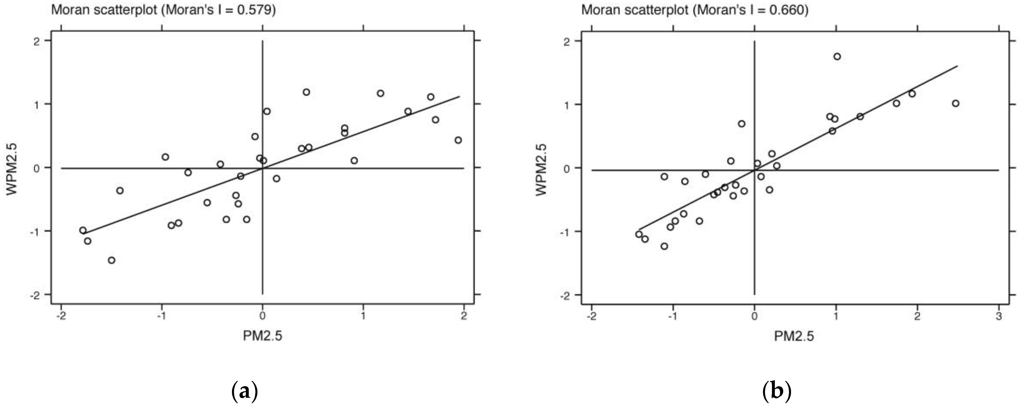
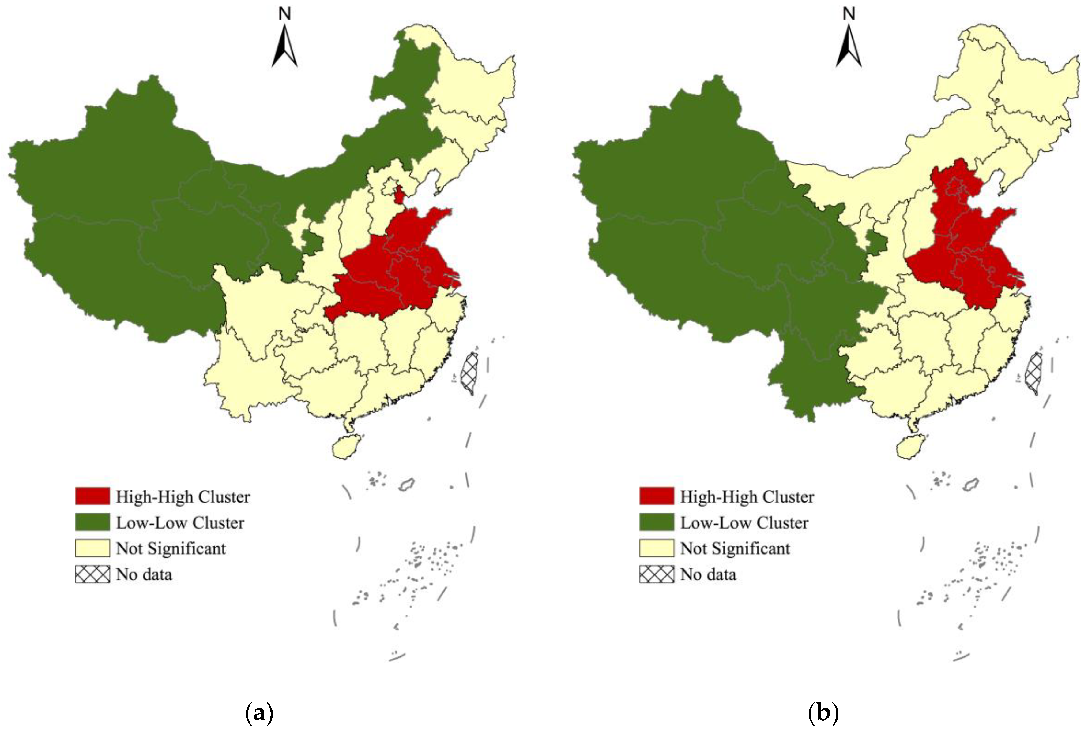
4.1. Spatial Autocorrelation of PM_2.5 Concentrations

The bivariate Moran scatterplots of the PM_2.5 concentrations in China are displayed in Figure 3. For simplicity, only the scatterplots of PM_2.5 concentrations for the years 1999 and 2016 are shown. In each scatterplot, the X axis represents the original variable PM_2.5, and the Y axis represents the spatially lagged variable WPM_2.5. The upper right (high-high clusters) and lower left (low-low clusters) quadrants indicate positive spatial autocorrelation, while the upper left (low-high clusters) and lower right (high-low clusters) quadrants indicate negative spatial autocorrelation. As shown in Figure 3, there is a significant and positive spatial autocorrelation for PM_2.5 concentrations, with the global Moran’s I equaling 0.579 and 0.660 in 1999 and 2016, respectively. Cluster maps, showing the clusters and outliers of PM_2.5 concentrations for 1999 and 2016, are given as well (see Figure 4). High-high clusters are located in the Bohai Rim region, the Yangtze River Delta region, and parts of the Central Plain region. Low-low clusters are located in the western part of China. The scatterplots and cluster maps confirm the existence of spatial autocorrelation. Therefore, spatial econometric models, considering spatial lags, should be employed.

4.2. Main Results of Spatial Econometric Analysis

Correct specification is crucial, since each spatial specification produces rather different interpretations. Diagnostic tests were used to select the preferred specification. The spatial dependences, in the form of a spatially lagged dependent variable or spatial error autocorrelation, were diagnosed by Lagrange multiplier tests [44]. Meanwhile, spatial and/or time specific effects were considered in different specifications. As shown in

Table 2. LM and robust LM tests for the spatial lag model and spatial error model.

Test	Matrix	Ordinary Least-Squares Regression	Spatial Specific Effect	Time Specific Effect	Spatial and Time Specific Effect
LM test for SLM	Wbin	239.997 *** [0.000]	435.172 *** [0.000]	155.377 *** [0.000]	166.011 *** [0.000]
	Wdis	105.332 *** [0.000]	1114.720 *** [0.000]	19.519 *** [0.000]	55.217 *** [0.000]
Robust LM test for SLM	Wbin	63.845 *** [0.000]	126.061 *** [0.000]	147.067 *** [0.000]	10.040 *** [0.002]
	Wdis	0.093 [0.761]	433.374 *** [0.000]	34.245 *** [0.000]	17.246 *** [0.000]
LM test for SEM	Wbin	178.141 *** [0.000]	351.054 *** [0.000]	49.768 *** [0.000]	159.082 *** [0.000]
	Wdis	124.955 *** [0.000]	801.318 *** [0.000]	1.908 [0.167]	50.552 *** [0.000]
Robust LM test for SEM	Wbin	1.989 [0.159]	41.943 *** [0.000]	41.459 *** [0.000]	3.110 * [0.078]
	Wdis	19.715 *** [0.000]	119.971 *** [0.000]	16.634 *** [0.000]	12.581 *** [0.000]

Note: p–values are given in brackets. *** significant at 1%; ** significant at 5%; * significant at 10%.

, the results obtained for the two weight matrices show strong spatial dependence, regardless of whether spatial and/or time specific effects are involved. Almost all of the (robust) Lagrange Multiplier tests for spatial lag and error dependence reject the null hypothesis of no spatial dependence, which points to the spatial Durbin model as the favorite specification [43].

The testing procedure in Yesilyurt and Elhorst [42] was used to identify the weight matrix that best fits the data. The binary contiguity matrix was identified as the most likely spatial weight matrix in our study. Since the dynamic spatial Durbin model produces the global spillover effects of PM_2.5 concentrations, it is more likely to occur in combination with a sparse weight matrix with only a limited number of non-zero elements. Our analysis concentrates on the estimation results of the dynamic spatial Durbin model in combination with the binary contiguity matrix. The inverse-distance weight matrix was used to check the robustness of our estimation results.

The estimation results of the dynamic SDM in combination with the binary contiguity weight matrix are reported in

Table 3. Results of the dynamic SDM for the full sample, with the binary contiguity matrix.

Variable	Coef.	Variable	Coef.	Short-Term Effects			Long-Term Effects
				Direct	Spillover	Total	Direct	Spillover	Total
WYt	0.614 *** (0.040)
Yt−1	0.364 *** (0.041)
WYt−1	−0.266 *** (0.065)
RFV	−0.006 (0.005)	WRFV	−0.020 ** (0.010)	−0.011 ** (0.006)	−0.058 *** (0.022)	−0.069 *** (0.026)	−0.016 * (0.008)	−0.077 ** (0.031)	−0.093 *** (0.035)
RGE	−0.009 (0.035)	WRGE	−0.089 (0.071)	−0.029 (0.034)	−0.218 (0.153)	−0.248 (0.165)	−0.040 (0.053)	−0.294 (0.211)	−0.334 (0.226)
NC	0.006 (0.021)	WNC	0.052 (0.041)	0.018 (0.022)	0.139 (0.091)	0.158 (0.102)	0.025 (0.033)	0.187 (0.125)	0.212 (0.139)
LGDP	−0.027 (0.038)	WLGDP	−0.227 *** (0.069)	−0.077 ** (0.041)	−0.579 *** (0.154)	−0.656 *** (0.175)	−0.106 * (0.062)	−0.776 *** (0.215)	−0.882 *** (0.243)
STG	−0.021 (0.039)	WSTG	−0.028 (0.065)	−0.030 (0.047)	−0.090 (0.160)	−0.120 (0.188)	−0.045 (0.070)	−0.117 (0.214)	−0.162 (0.253)
R2	0.194
Obs.	510

Note: Standard errors are given in parentheses. *** significant at 1%; ** significant at 5%; * significant at 10%.

. The estimates of the coefficients are given in columns 2 and 4. Estimates of the direct effects and spillover effects, as well as the total effects, are given in columns 5–10. The coefficient of the endogenous spatial lag is 0.614 and is significant at the 1% level. There exist strong global spillover effects—that is, the PM_2.5 concentration in a province is positively affected by the PM_2.5 concentrations in other provinces, even if they are not neighbors. This can be explained by the long-range transmission of particulate matter. The estimates of coefficients show significant internal habit persistence. The PM_2.5 concentration depends on its value in the previous year; the coefficient τ accounts for 0.364 and is highly significant. There is strong evidence of external habit persistence as well; the coefficient of the PM_2.5 in neighboring provinces in the previous year takes a value of −0.266 and is also significant at the 1% level. To investigate whether the dynamic SDM could be replaced by a simpler model (dynamic SLM, dynamic SEM or static SDM), likelihood ratio tests were performed. The results indicate that the null hypothesis of a dynamic SLM (LR = 15.47, with 5 degrees of freedom [df], p = 0.009) or a dynamic SEM (LR = 18.76, 5 df, p = 0.002) is rejected. The hypothesis that the coefficients of internal and external habit persistence are jointly insignificant is rejected as well (LR = 79.97, 2 df, p = 0.000).

The direct effects of the freight transport variable are negative and significant both in the short term and long term, implying that PM_2.5 concentrations decrease with the modal shift of freight from road to rail. The direct effects of the log of real GDP per capita are negative and significant as well. PM_2.5 concentrations decrease with economic growth in a province. When a quadratic term of the log of real GDP per capita was added to the model, the coefficient of the quadratic term was insignificant. It indicates that there is no evidence of a nonlinear relationship between PM_2.5 concentrations and economic growth. The results of this specification are not given, since the coefficients of other variables remain almost unchanged. The spillover effects of the freight transport variable and the GDP per capita is negative and significant at the 1% level in the short term, but their magnitudes are larger than the direct effects. The spillover effects of the two explanatory variables exhibit similar significance levels in the long term. The PM_2.5 concentrations do not only decrease with the road-to-rail freight modal shift and the level of GDP in a province, but also and to a larger extent with those in neighboring provinces. The directions of the effects of other explanatory variables are in line with our expectation. The short-term and long-term spillover effects of road congestion are positive and weakly significant (p < 0.15), implying that road congestion in a province contributes to other provinces’ PM_2.5 concentrations. As another contributing factor, energy efficiency has negative and weakly significant spillover impacts (p < 0.15). The direct and spillover effects of trade openness are negative but insignificant.

The specification, shown in column 2 of

Table 4. Results of the dynamic SDM with an interaction term between a freight modal shift and energy efficiency.

Variable	Full Sample		BR	YRD-PRD	CP	W
	(1)	(2)
WYt	0.618 *** (0.040)	0.616 *** (0.040)	0.230 * (0.135)	0.005 (0.102)	0.034 (0.118)	0.441 *** (0.064)
Yt−1	0.361 *** (0.041)	0.359 *** (0.041)	−0.216 ** (0.095)	−0.075 (0.088)	−0.017 (0.072)	0.265 *** (0.061)
WYt−1	−0.252 *** (0.065)	−0.264 *** (0.065)	−0.428 ** (0.204)	−0.186 (0.137)	0.134 (0.132)	−0.201 ** (0.090)
RFV		0.007 (0.008)	−0.045 ** (0.018)	−0.703 *** (0.259)	−0.027 (0.038)	0.054 *** (0.020)
RFV*RGE	−0.010 ** (0.005)	−0.016 ** (0.008)	0.047 *** (0.017)	0.663 ** (0.269)	0.002 (0.043)	−0.111 *** (0.036)
RGE	0.033 (0.041)	0.050 (0.045)	−0.148 (0.095)	−0.158 (0.185)	0.138 (0.131)	−0.073 (0.103)
NC	0.001 (0.021)	0.001 (0.021)	0.097 * (0.053)	−0.039 (0.059)	0.145 ** (0.063)	0.060 (0.041)
LGDP	−0.040 (0.037)	−0.026 (0.038)	0.302 *** (0.093)	−0.249 * (0.147)	0.242 * (0.143)	−0.245 *** (0.079)
STG	−0.011 (0.040)	−0.002 (0.040)	−0.077 (0.056)	−0.225 ** (0.090)	−1.084 ** (0.520)	0.134 (0.199)
LPMN			0.501 *** (0.068)	0.088 (0.108)	0.893 *** (0.101)	0.385 *** (0.080)
WRFV		−0.035 *** (0.013)	−0.002 (0.038)	−0.515 (0.441)	0.255 *** (0.080)	0.083 (0.054)
WRFV*RGE	−0.005 (0.010)	0.018 (0.013)	0.011 (0.036)	0.762 * (0.470)	−0.260 *** (0.090)	−0.225 ** (0.091)
WRGE	−0.151 ** (0.078)	−0.168 ** (0.081)	−0.032 (0.168)	0.157 (0.279)	0.154 (0.372)	0.448 ** (0.221)
WNC	0.020 (0.041)	0.065 (0.044)	0.122 (0.105)	0.179 * (0.093)	−0.143 (0.124)	0.085 (0.089)
WLGDP	−0.182 *** (0.067)	−0.223 *** (0.069)	−0.193 (0.247)	−0.681 ** (0.294)	−0.644 * (0.364)	−0.574 *** (0.177)
WSTG	−0.015 (0.068)	−0.074 (0.071)	−0.161 (0.113)	−0.290 * (0.163)	−0.629 (0.743)	0.187 (0.479)
R2	0.156	0.196	0.298	0.288	0.252	0.106
Obs.	510	510	85	102	102	221

Note: Standard errors are given in parentheses. *** significant at 1%; ** significant at 5%; * significant at 10%.

, replaces the freight transport variable by the product between the modal shift of freight transport and energy efficiency. The coefficient of the interaction term is negative (−0.010) and significant at the 5% level. The coefficient of the spatially lagged interaction term takes a negative value of −0.005 but is insignificant. This specification yields negative and significant coefficients for the spatially lagged energy efficiency and (log of) real GDP per capita. The significance of the interaction term may be the result of the omission of other relevant factors, in particular, the freight transport variable by itself. Therefore, it is necessary to include the freight modal shift and energy efficiency individually alongside their product. The results of this specification, given in column 3 of Table 4, show that the coefficient on the modal shift of freight transport is positive but insignificant, while the coefficient on the interaction term is negative and significant. The results indicate that the interaction between a road-to-rail freight modal shift and energy efficiency leads to a decrease of PM_2.5 concentrations in a province. The coefficient of the spatially lagged modal shift of freight transport is negative and highly significant at the 1% level. However, the coefficient of the spatially lagged interaction term is positive and insignificant.

To investigate whether the spillover effects of the interaction term were influenced by the heterogeneity in the exogenous spatial dependence across different regions of China, the panel data used in this study were divided into four subsamples (i.e., the BR region, the YRD-PRD region, the CP region and the W region). The dynamic spatial Durbin models, incorporating the temporal and space-time lags of the dependent variable, were employed for the subsamples. The estimation results are reported in columns 4–7 of Table 4. As shown in columns 4 and 5, significant changes occur in the BR and the YRD-PRD subsamples. The coefficients of the interaction term are positive and significant. In the YRD-PRD subsample, the coefficient of the spatially lagged interaction term is positive and significant as well. The results indicate that the interaction between a road-to-rail freight modal shift and energy efficiency may lead to an increase in the PM_2.5 concentrations in the BR and YRD-PRD regions. The descriptive statistics, given in Table 1, offer clues to these findings. Due to the lower energy intensities in these two regions, especially the YRD-PRD region, a road-to-rail freight modal shift cannot reduce energy consumption anymore. The estimation results for the CP and the W subsamples are given in columns 6 and 7. The coefficients of the spatially lagged interaction term in these two subsamples are negative and highly significant. Moreover, the results for the W subsample indicate a negative and significant coefficient of the interaction term. The interaction between a freight modal shift and energy efficiency leads to a decrease in the PM_2.5 concentrations in these two regions, especially in the W region. The coefficients of the spatially lagged (log of) real GDP per capita are negative and significant in three of the subsamples, indicating that PM_2.5 concentrations decrease with the economic growth of other provinces in the region. The coefficients of the log of real GDP per capita are negative and significant in the YRD-PRD and W subsamples, but are positive and significant in the BR and CP subsamples. The heterogeneous effects of economic growth across different regions may be the reason for the insignificant coefficient in the full sample.

4.3. Robustness Checks

We report and discuss the results of three robustness checks. The first check replaced the spatial weight matrix by the inverse-distance matrix and re-estimated the dynamic SDM, where an interaction term between a freight modal shift and energy efficiency was included. Estimations for the full sample are given in column 2 of

Table 5. Results of the robustness checks, with the inverse-distance weight matrix and subsamples characterized by the average value of energy efficiency.

Variable	Wdis					Wbin
	Full Sample	BR	YRD-PRD	CP	W	LE Subsample	HE Subsample
WYt	0.639 *** (0.077)	0.416 ** (0.201)	0.479 ** (0.197)	0.809 *** (0.253)	0.394 *** (0.122)	0.444 *** (0.063)	0.307 *** (0.064)
Yt−1	0.405 *** (0.044)	−0.294 *** (0.099)	−0.048 (0.101)	−0.021 (0.081)	0.275 *** (0.061)	0.285 *** (0.061)	0.190 *** (0.055)
WYt−1	−0.991 *** (0.244)	−0.398 (0.445)	−0.335 (0.347)	0.115 (0.459)	−0.479 * (0.248)	−0.123 (0.085)	−0.197 ** (0.089)
RFV	−0.002 (0.010)	−0.015 (0.028)	−0.671 * (0.357)	0.067 (0.043)	0.088 *** (0.025)	0.066 *** (0.019)	−0.037 ** (0.015)
RFV*RGE	−0.005 (0.009)	0.035 (0.029)	0.622 * (0.387)	−0.155 *** (0.045)	−0.179 *** (0.042)	−0.110 *** (0.035)	0.020 (0.013)
RGE	−0.036 (0.046)	−0.325 * (0.180)	0.204 (0.269)	−0.149 (0.246)	0.045 (0.119)	0.007 (0.103)	0.010 (0.067)
NC	0.028 (0.023)	0.041 (0.072)	0.011 (0.074)	−0.048 (0.105)	0.083 (0.054)	0.086 * (0.048)	0.007 (0.028)
LGDP	−0.089 ** (0.043)	0.079 (0.154)	0.139 (0.211)	0.344 (0.253)	−0.508 *** (0.117)	−0.097 (0.073)	−0.017 (0.056)
STG	−0.025 (0.048)	−0.182 (0.131)	−0.402 *** (0.125)	−1.598 ** (0.741)	0.303 (0.247)	0.113 (0.250)	−0.059 (0.043)
LPMN		0.526 *** (0.063)	0.200 ** (0.098)	0.854 *** (0.086)	0.493 *** (0.085)	0.288 *** (0.081)	0.276 *** (0.064)
WRFV	−0.057 (0.058)	0.121 (0.106)	−0.365 (1.243)	0.719 *** (0.223)	0.356 *** (0.133)	0.085 ** (0.041)	0.020 (0.024)
WRFV*RGE	0.042 (0.047)	−0.065 (0.105)	0.486 (1.437)	−0.965 *** (0.242)	−0.703 *** (0.209)	−0.163 ** (0.079)	0.003 (0.019)
WRGE	−0.576 * (0.299)	−0.414 (0.503)	1.365 (0.861)	−0.989 (1.135)	0.789 (0.591)	0.256 (0.179)	−0.114 (0.117)
WNC	0.471 ** (0.185)	−0.109 (0.172)	0.295 (0.259)	−0.689 * (0.405)	0.155 (0.316)	0.106 * (0.065)	0.043 (0.047)
WLGDP	−1.187 *** (0.302)	−0.618 (0.557)	0.410 (0.647)	−0.023 (1.161)	−1.843 ** (0.723)	−0.064 (0.087)	−0.027 (0.102)
WSTG	−0.470 (0.298)	−0.282 (0.366)	−1.007 ** (0.426)	−3.350 (2.551)	1.631 (1.356)	0.561 (0.441)	−0.129 ** (0.062)
R2	0.324	0.409	0.084	0.168	0.136	0.260	0.511
Obs.	510	85	102	102	221	238	272

Note: Standard errors are given in parentheses. *** significant at 1%; ** significant at 5%; * significant at 10%.

. The coefficients of the interaction term and the spatially lagged interaction term are insignificant.

To further check the robustness of the heterogeneous impacts of the freight modal shift, we re-estimated the dynamic SDM for the four subsamples using the inverse-distance matrix. The results were summarized in columns 3–6 of Table 5. As expected, the coefficients of the interaction term, as well as the coefficients of the spatially lagged interaction term, are negative and significant in the CP and W subsamples. In these two regions, shifting from road to rail freight transport interacts with energy efficiency to reduce PM_2.5 concentrations. However, in the BR and YRD-PRD regions, there is no evidence that through the energy channel the modal shift of freight from road to rail may be beneficial for the environment [45]. In our second robustness check, we divided the full sample into two subsamples characterized by the average value of energy efficiency and re-estimated the dynamic SDM using the binary contiguity matrix. The estimation results for the lower energy efficiency (LE) subsample, which includes provinces with an average energy efficiency lower than 0.844, are shown in column 7 of Table 5. The coefficient of the interaction term is −0.110 and significant, and the coefficient of the spatially lagged interaction term is negative (−0.163) and significant as well. The estimation results for the higher energy efficiency (HE) subsample, which includes provinces with an average energy efficiency greater than 0.844, are shown in the last column of Table 5. The coefficients of the interaction term are positive and insignificant. The heterogeneity in the exogenous spatial dependence is confirmed by the finding that provinces with higher energy intensities gain more environmental benefits from the interaction between a freight modal shift and energy efficiency.

Finally, we tested whether the results for the four subsamples were robust in changing the set of explanatory variables. Urbanization or industrialization was incorporated into the dynamic SDM. The results of these two specifications for the four subsamples are summarized in

Table 6. Results of robustness checks, with additional variables.

Variable	BR		YRD-PRD		CP		W
	(1)	(2)	(1)	(2)	(1)	(2)	(1)	(2)
WYt	0.236 * (0.134)	0.230 * (0.132)	0.005 (0.102)	0.009 (0.102)	0.011 (0.119)	0.021 (0.119)	0.457 *** (0.064)	0.435 *** (0.064)
Yt−1	−0.210 ** (0.094)	−0.237 *** (0.090)	−0.075 (0.089)	−0.066 (0.087)	0.017 (0.071)	0.029 (0.077)	0.249 *** (0.062)	0.252 *** (0.062)
WYt−1	−0.434 ** (0.203)	−0.450 ** (0.193)	−0.187 (0.140)	−0.095 (0.145)	0.224 * (0.139)	0.115 (0.143)	−0.174 * (0.091)	−0.208 ** (0.090)
RFV	−0.055 *** (0.019)	−0.055 *** (0.017)	−0.688 ** (0.290)	−0.703 *** (0.257)	−0.024 (0.037)	−0.016 (0.038)	0.052 ** (0.021)	0.054 ** (0.021)
RFV*RGE	0.054 *** (0.018)	0.042 *** (0.016)	0.646 ** (0.303)	0.670 *** (0.267)	0.008 (0.042)	−0.002 (0.043)	−0.108 *** (0.036)	−0.108 *** (0.036)
RGE	−0.109 (0.097)	−0.078 (0.092)	−0.155 (0.188)	−0.215 (0.194)	0.126 (0.128)	0.177 (0.132)	−0.060 (0.104)	−0.125 (0.114)
NC	0.100 ** (0.052)	0.146 *** (0.053)	−0.041 (0.062)	−0.006 (0.061)	0.127 ** (0.062)	0.175 *** (0.066)	0.061 (0.042)	0.043 (0.043)
LGDP	0.290 *** (0.091)	0.360 *** (0.089)	−0.245 * (0.150)	0.071 (0.244)	0.276 ** (0.140)	0.153 (0.189)	−0.266 *** (0.087)	−0.258 ** (0.108)
STG	−0.060 (0.056)	−0.040 (0.053)	−0.222 ** (0.093)	−0.249 *** (0.091)	−0.766 (0.523)	−1.143 ** (0.522)	0.100 (0.200)	0.149 (0.199)
SUP	0.430 (0.303)		0.016 (0.124)		0.611 (0.449)		−0.064 (0.108)
SSG		−0.707 *** (0.238)		−0.868 (0.572)		0.015 (0.222)		−0.064 (0.277)
LPMN	0.506 *** (0.067)	0.519 *** (0.064)	0.089 (0.110)	0.077 (0.107)	0.852 *** (0.100)	0.928 *** (0.102)	0.368 *** (0.085)	0.370 *** (0.083)
WRFV	−0.011 (0.038)	−0.013 (0.036)	−0.480 (0.544)	−0.570 (0.441)	0.322 *** (0.086)	0.248 *** (0.083)	0.080 (0.054)	0.098 * (0.056)
WRFV*RGE	0.017 (0.035)	−0.006 (0.034)	0.725 (0.582)	0.818 * (0.475)	−0.321 *** (0.095)	−0.226 ** (0.093)	−0.228 ** (0.091)	−0.240 *** (0.092)
WRGE	0.031 (0.171)	0.090 (0.162)	0.168 (0.301)	−0.031 (0.336)	0.403 (0.374)	0.266 (0.376)	0.500 ** (0.231)	0.539 ** (0.259)
WNC	0.103 (0.104)	0.244 ** (0.107)	0.177 * (0.095)	0.207 ** (0.102)	−0.106 (0.122)	−0.075 (0.136)	0.102 (0.090)	0.059 (0.095)
WLGDP	−0.130 (0.245)	−0.392 (0.260)	−0.676 ** (0.297)	−0.172 (0.417)	−0.900 ** (0.368)	−1.129 ** (0.530)	−0.610 *** (0.186)	−0.470 ** (0.198)
WSTG	−0.107 (0.119)	−0.153 (0.106)	−0.284 * (0.170)	−0.410 ** (0.178)	−0.926 (0.731)	−0.772 (0.755)	0.196 (0.480)	0.121 (0.490)
WSUP	0.459 (0.437)		0.022 (0.225)		2.387 ** (0.975)		0.330 (0.263)
WSSG		−1.246 ** (0.617)		−0.826 (0.724)		0.857 (0.709)		−0.662 (0.531)
R2	0.414	0.178	0.290	0.109	0.555	0.091	0.115	0.104
Obs.	85	85	102	102	102	102	221	221

Note: Standard errors are given in parentheses. *** significant at 1%; ** significant at 5%; * significant at 10%.

. The coefficient estimates of other explanatory variables, and especially those of the interaction term, change only slightly. Again, the results confirm the spatial heterogeneity in the interaction effects between the modal shift of freight transport and energy efficiency.

5. Conclusions

In this study, we have sought to gain a better understanding of the spatial dependence and heterogeneity of PM_2.5 concentrations. The impacts of a road-to-rail freight modal shift on PM_2.5 concentrations were estimated by employing the dynamic spatial Durbin model. The spillover effects of the freight modal shift, as well as the direct effects, exist both in the short and long term. PM_2.5 concentrations do not only decrease with a modal shift of freight from road to rail in a province, but also and to a larger extent with that in neighboring provinces. The estimates of coefficients show significant internal and external habit persistence, as well as endogenous spatial dependence. To investigate the channel through which the modal shift of freight transport might be beneficial for the environment, we enriched the specification by including the interaction term between freight modal shift and energy efficiency. However, results show that there is heterogeneity in the exogenous spatial dependence across different regions of China. The modal shift of freight from road to rail interacts with energy efficiency to reduce the PM_2.5 concentrations, but only in the central and western regions. The heterogeneity in the interaction effects between a freight modal shift and energy efficiency could be explained by the different energy intensities in these regions. The findings are confirmed by three robustness checks. Economic growth has significant impacts on PM_2.5 concentrations as well. Generally, PM_2.5 concentrations decrease with the real GDP per capita in neighboring provinces, although the direct effects of real GDP per capita are different across China’s four economic zones. However, EKC does not exist since there is no evidence for the nonlinear relationship between PM_2.5 concentrations and economic growth. Further studies are needed to explore the heterogeneous effects of economic growth on PM_2.5 concentrations.

From the perspective of government policies directed toward sustainable development, the results suggest important determinants to focus on. Specifically, the government must act on the modal shift of freight transport, which might generate both direct and spatial spillover effects on PM_2.5 concentrations. It is essential because the environmental benefits of a freight modal shift are partly transferred to neighboring provinces. In the central and western regions of China, provinces that hope to reduce PM_2.5 concentrations should shift freight transport from road to rail and increase the energy efficiency in the transportation industry. In addition, the improved technology and modal shifting measures must make absolute reductions in the total energy consumption, rather than merely improve the energy efficiency of the transport sector. Meanwhile, the transportation energy use of various commodities should be considered when shifting freight transport modes. The highest priority should be given to the freight modal shift of long-distance heavy items. Additional polices aimed at reducing road congestion or promoting trade openness and economic growth are needed as well.

References

1. Huang, R.J.; Zhang, Y.; Bozzetti, C.; Ho, K.F.; Cao, J.J.; Han, Y.; Daellenbach, K.R.; Slowik, J.G.; Platt, S.M.; Canonaco, F.; et al. High secondary aerosol contribution to particulate pollution during haze events in China. Nature 2014, 514, 218–222. [Google Scholar] [CrossRef] [PubMed] [Green Version]
2. Bell, M.L.; Dominici, F.; Ebisu, K.; Zeger, S.L.; Samet, J.M. Spatial and temporal variation in PM2.5 chemical composition in the United States for health effects studies. Environ. Health Perspect. 2007, 115, 989–995. [Google Scholar] [CrossRef] [PubMed]
3. Xie, Y.; Dai, H.; Dong, H.; Hanaoka, T.; Masui, T. Economic impacts from PM2.5 pollution-related health effects in China: A provincial-level analysis. Environ. Sci. Technol. 2016, 50, 4836–4843. [Google Scholar] [CrossRef] [PubMed]
4. Chapman, L. Transport and climate change: A review. J. Transp. Geogr. 2007, 15, 354–367. [Google Scholar] [CrossRef]
5. Lang, J.; Zhang, Y.; Zhou, Y.; Cheng, S.; Chen, D.; Guo, X.; Chen, S.; Li, X.; Xing, X.; Wang, H. Trends of PM2.5 and chemical composition in Beijing, 2000–2015. Aerosol. Air Qual. Res. 2017, 17, 412–425. [Google Scholar] [CrossRef]
6. Fang, C.; Zhang, Z.; Jin, M.; Zou, P.; Wang, J. Pollution characteristics of PM2.5 aerosol during haze periods in Changchun, China. Aerosol. Air Qual. Res. 2017, 17, 888–895. [Google Scholar] [CrossRef]
7. Rupasingha, A.; Goetz, S.J.; Debertin, D.L.; Pagoulatos, A. The environmental Kuznets curve for US counties: A spatial econometric analysis with extensions. Pap. Reg. Sci. 2004, 83, 407–424. [Google Scholar] [CrossRef]
8. Auffhammer, M.; Carson, R.T. Forecasting the path of China’s CO2 emissions using province-level information. J. Environ. Econ. Manag. 2008, 55, 229–247. [Google Scholar] [CrossRef]
9. Diao, X.D.; Zeng, S.X.; Tam, C.M.; Tam, V.W.Y. EKC analysis for studying economic growth and environmental quality: A case study in China. J. Clean. Prod. 2009, 17, 541–548. [Google Scholar] [CrossRef]
10. Halkos, G.E.; Paizanos, E.A. The effect of government expenditure on the environment: An empirical investigation. Ecol. Econ. 2013, 91, 48–56. [Google Scholar] [CrossRef] [Green Version]
11. Xu, B.; Lin, B. Factors affecting carbon dioxide (CO2) emissions in China’s transport sector: A dynamic nonparametric additive regression model. J. Clean. Prod. 2015, 101, 311–322. [Google Scholar] [CrossRef]
12. Lin, G.; Fu, J.; Jiang, D.; Hu, W.; Dong, D.; Huang, Y.; Zhao, M. Spatio-temporal variation of PM2.5 concentrations and their relationship with geographic and socioeconomic factors in China. Int. J. Environ. Res. Public Health 2014, 11, 173–186. [Google Scholar] [CrossRef] [PubMed]
13. Ma, Y.; Ji, Q.; Fan, Y. Spatial linkage analysis of the impact of regional economic activities on PM2.5 pollution in China. J. Clean. Prod. 2016, 139, 1157–1167. [Google Scholar] [CrossRef]
14. Wu, J.; Zhang, P.; Yi, H.; Qin, Z. What causes haze pollution? An empirical study of PM2.5 concentrations in Chinese cities. Sustainability 2016, 8, 132. [Google Scholar] [CrossRef]
15. Ang, B.W. The LMDI approach to decomposition analysis: A practical guide. Energy Policy 2005, 33, 867–871. [Google Scholar] [CrossRef]
16. Rose, A.; Casler, S. Input-output structural decomposition analysis: A critical appraisal. Econ. Syst. Res. 1996, 8, 33–62. [Google Scholar] [CrossRef]
17. Guan, D.; Su, X.; Zhang, Q.; Peters, G.P.; Liu, Z.; Lei, Y.; He, K. The socioeconomic drivers of China’s primary PM2.5 emissions. Environ. Res. Lett. 2014, 9, 024010. [Google Scholar] [CrossRef]
18. Chan, C.K.; Yao, X. Air pollution in mega cities in China. Atmos. Environ. 2008, 42, 1–42. [Google Scholar] [CrossRef]
19. Maddison, D. Environmental Kuznets curves: A spatial econometric approach. J. Environ. Econ. Manag. 2006, 51, 218–230. [Google Scholar] [CrossRef]
20. Hosseini, H.M.; Kaneko, S. Can environmental quality spread through institutions? Energy Policy 2013, 56, 312–321. [Google Scholar] [CrossRef]
21. Li, Q.; Song, J.; Wang, E.; Hu, H.; Zhang, J.; Wang, Y. Economic growth and pollutant emissions in China: A spatial econometric analysis. Stoch. Environ. Res. Risk Assess. 2014, 28, 429–442. [Google Scholar] [CrossRef]
22. Fang, C.; Liu, H.; Li, G.; Sun, D.; Miao, Z. Estimating the impact of urbanization on air quality in China using spatial regression models. Sustainability 2015, 7, 15570–15592. [Google Scholar] [CrossRef]
23. Hao, Y.; Liu, Y. The influential factors of urban PM2.5 concentrations in China: A spatial econometric analysis. J. Clean. Prod. 2016, 112, 1443–1453. [Google Scholar] [CrossRef]
24. Forkenbrock, D.J. Comparison of external costs of rail and truck freight transportation. Transp. Res. Part A 2001, 35, 321–337. [Google Scholar] [CrossRef] [Green Version]
25. Janic, M. Modelling the full costs of an intermodal and road freight transport network. Transp. Res. D Transp. Environ. 2007, 12, 33–44. [Google Scholar] [CrossRef]
26. Van Donkelaar, A.; Martin, R.V.; Brauer, M.; Hsu, N.C.; Kahn, R.A.; Levy, R.C.; Lyapustin, A.; Sayer, M.; Winker, D.M. Global estimates of fine particulate matter using a combined geophysical-statistical method with information from satellites, models, and monitors. Environ. Sci. Technol. 2016, 50, 3762–3772. [Google Scholar] [CrossRef] [PubMed]
27. Woodburn, A.G. A logistical perspective on the potential for modal shift of freight from road to rail in Great Britain. Int. J. Transp. Manag. 2003, 1, 237–245. [Google Scholar] [CrossRef] [Green Version]
28. Yang, H.; Yu, J.Z.; Ho, S.S.H.; Xu, J.; Wu, W.S.; Wan, C.H.; Wang, X.; Wang, X.; Wang, L. The chemical composition of inorganic and carbonaceous materials in PM2.5 in Nanjing, China. Atmos. Environ. 2005, 39, 3735–3749. [Google Scholar] [CrossRef]
29. Aldabe, J.; Elustondo, D.; Santamaría, C.; Lasheras, E.; Pandolfi, M.; Alastuey, A.; Querol, X.; Santamaría, J.M. Chemical characterisation and source apportionment of PM2.5 and PM10 at rural, urban and traffic sites in Navarra (North of Spain). Atmos. Res. 2011, 102, 191–205. [Google Scholar] [CrossRef]
30. Tong, H.Y.; Hung, W.T.; Cheung, C.S. On-road motor vehicle emissions and fuel consumption in urban driving conditions. J. Air Waste Manag. Assoc. 2000, 50, 543–554. [Google Scholar] [CrossRef] [PubMed]
31. Brook, J.R.; Dann, T.F.; Burnett, R.T. The relationship among TSP, PM10, PM2.5, and inorganic constituents of atmospheric participate matter at multiple Canadian locations. J. Air Waste Manag. Assoc. 1997, 47, 2–19. [Google Scholar] [CrossRef]
32. Grossman, G.M.; Krueger, A.B. Economic growth and the environment. Q. J. Econ. 1995, 110, 353–377. [Google Scholar] [CrossRef]
33. Park, S.; Lee, Y. Regional model of EKC for air pollution: Evidence from the Republic of Korea. Energy Policy 2011, 39, 5840–5849. [Google Scholar] [CrossRef]
34. Jakob, M.; Marschinski, R. Interpreting trade-related CO2 emission transfers. Nat. Clim. Chang. 2013, 3, 19–23. [Google Scholar] [CrossRef]
35. Meng, J.; Liu, J.; Guo, S.; Huang, Y.; Tao, S. The impact of domestic and foreign trade on energy-related PM emissions in Beijing. Appl. Energy 2016, 184, 853–862. [Google Scholar] [CrossRef]
36. Grossman, G.M.; Krueger, A.B. Environmental impacts of a North American free trade agreement. In The U.S.-Mexico Free Trade Agreement; Garber, P., Ed.; MIT Press: Cambridge, MA, USA, 1993; pp. 13–55. [Google Scholar]
37. Wang, S.; Zhou, C.; Wang, Z.; Feng, K.; Hubacek, K. The characteristics and drivers of fine particulate matter (PM2.5) distribution in China. J. Clean. Prod. 2017, 142, 1800–1809. [Google Scholar] [CrossRef]
38. Wang, S.; Hao, J. Air quality management in China: Issues, challenges, and options. J. Environ. Sci. 2012, 24, 2–13. [Google Scholar] [CrossRef]
39. Zhang, S.; Worrell, E.; Crijns-Graus, W.; Wagner, F.; Cofala, J. Co-benefits of energy efficiency improvement and air pollution abatement in the Chinese iron and steel industry. Energy 2014, 78, 333–345. [Google Scholar] [CrossRef]
40. Geller, H.; Schaeffer, R.; Szklo, A.; Tolmasquim, M. Policies for advancing energy efficiency and renewable energy use in Brazil. Energy Policy 2004, 32, 1437–1450. [Google Scholar] [CrossRef]
41. Anselin, L. Local indicators of spatial association–LISA. Geogr. Anal. 1995, 27, 93–115. [Google Scholar] [CrossRef]
42. Yesilyurt, M.E.; Elhorst, J.P. Impacts of neighboring countries on military expenditures: A dynamic spatial panel approach. J. Peace Res. 2017, 54, 777–790. [Google Scholar] [CrossRef]
43. LeSage, J.P.; Pace, R.K. Introduction to Spatial Econometrics; CRC Press: Boca Raton, FL, USA, 2009; pp. 155–185. [Google Scholar]
44. Anselin, L.; Bera, A.K.; Florax, R.; Yoon, M.J. Simple diagnostic tests for spatial dependence. Reg. Sci. Urban Econ. 1996, 26, 77–104. [Google Scholar] [CrossRef]
45. Vanek, F.M.; Morlok, E.K. Improving the energy efficiency of freight in the United States through commodity based analysis: justification and implementation. Transp. Res. D Transp. Environ. 2000, 5, 11–29. [Google Scholar] [CrossRef]
Figure 1. The shares of freight transport in road, railway, waterway, aviation and pipeline, 1985–2017. (Source: Raw data on the freight transport volume were collected from China’s National Bureau of Statistics; the shares of freight transport volume in the five modes were calculated by the authors).
Sustainability 10 02865 g001
Figure 2. China’s PM2.5 concentrations. (a) PM2.5 concentrations for 1999; (b) PM2.5 concentrations for 2016. (Source: PM2.5 grids were obtained from CIESIN at Columbia University; http://sedac.ciesin.columbia.edu/data/sets/).
Sustainability 10 02865 g002
Figure 3. Moran scatterplots of the PM2.5 concentrations in China. (a) Moran scatterplot of PM2.5 concentrations in 1999; (b) Moran scatterplot of PM2.5 concentrations in 2016.
Sustainability 10 02865 g003
Figure 4. Cluster maps of PM2.5 concentrations in China. (a) Cluster map of PM2.5 concentrations in 1999; (b) Cluster map of PM2.5 concentrations in 2016.
Sustainability 10 02865 g004