Multiple Types of Plug-In Charging Facilities’ Location-Routing Problem with Time Windows for Mobile Charging Vehicles

Abstract
1. Introduction
1.1. Motivation
1.2. Literature Review
1.3. Contribution of This Paper
- (1)
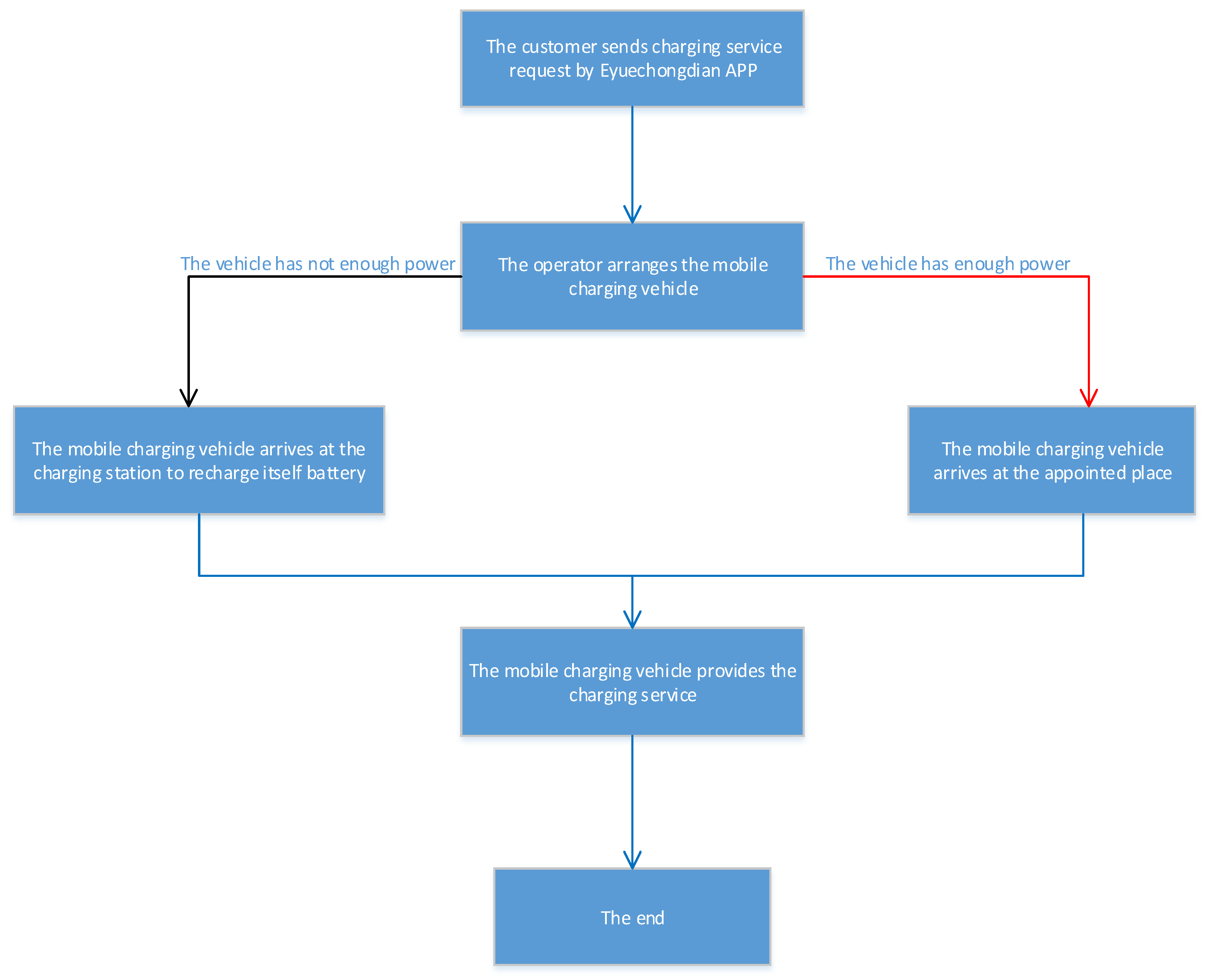
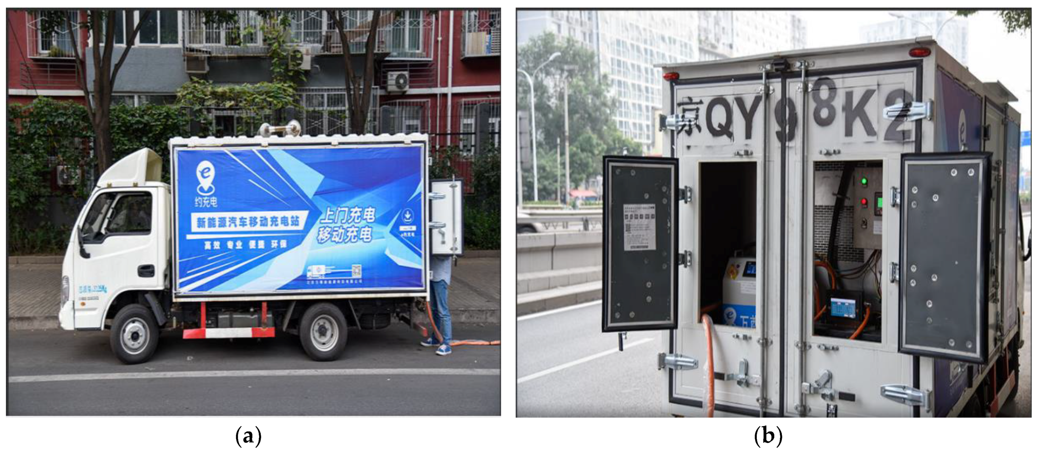
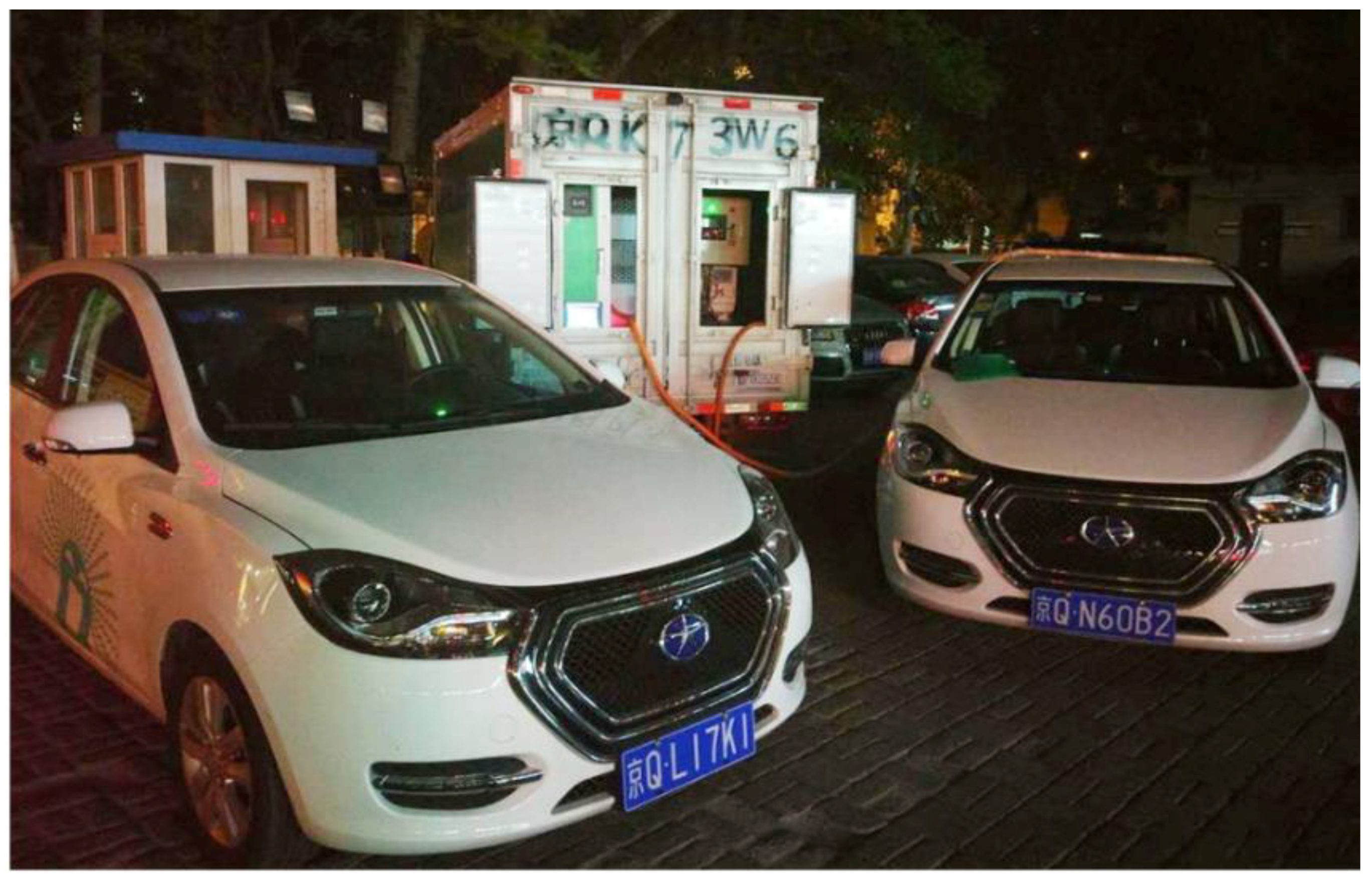
- In order to avoid the disadvantages of the traditional charging methods, namely only providing charging service in a fixed location, the novel charge replenishment is presented, in which the charging service can be provided by the MCVs, which could offer charging service at any time and location requested.
- (2)
- To avoid sub optimizing by separating the location and vehicle routing, we built the mobile charging service of the MCVs on the LRP to integrate two decision levels with the strategic level (location) and tactical level (routing).
- (3)
- Using the linearization skill, we formulate the mobile charging service of MCVs as the multiple types of plug-in charging facilities’ location-routing problem with time windows for mobile charging vehicles (MTPCF-LRPwTW-MCVs), and the model is formulated as a 0–1 mixed integer linear program (MILP) to ensure the accuracy of the solution.
- (4)
- Based on the work by Schneider et al. [47], a set of benchmark instances are designed to verify the correctness of the model and the efficiency of the solution.
- (5)
- Some reasonable sensitivity analyses are conducted to provide the operators of the MCVs with reasonable investment methods, such as the capacity of the battery of MCVs, the charging rate of the charging device, and so on.
1.4. Organization of This Paper
2. Problem Description
2.1. Notations
2.2. Problem Description
3. Optimization Framework
4. Numerical Experiments
4.1. Generation of MTPCF-LRPwTW-MCVs Benchmark Instances
4.2. Performance on All Instances
4.3. Sensitivity Analyses
4.3.1. The Sensitivity Analysis of Battery Capacity
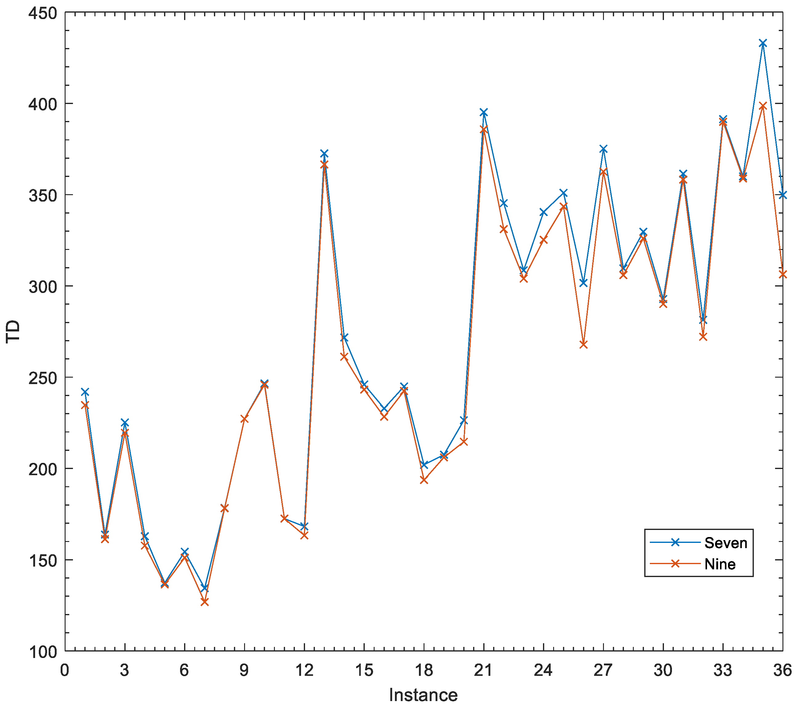
4.3.2. The Sensitivity Analysis of Recharging Rate
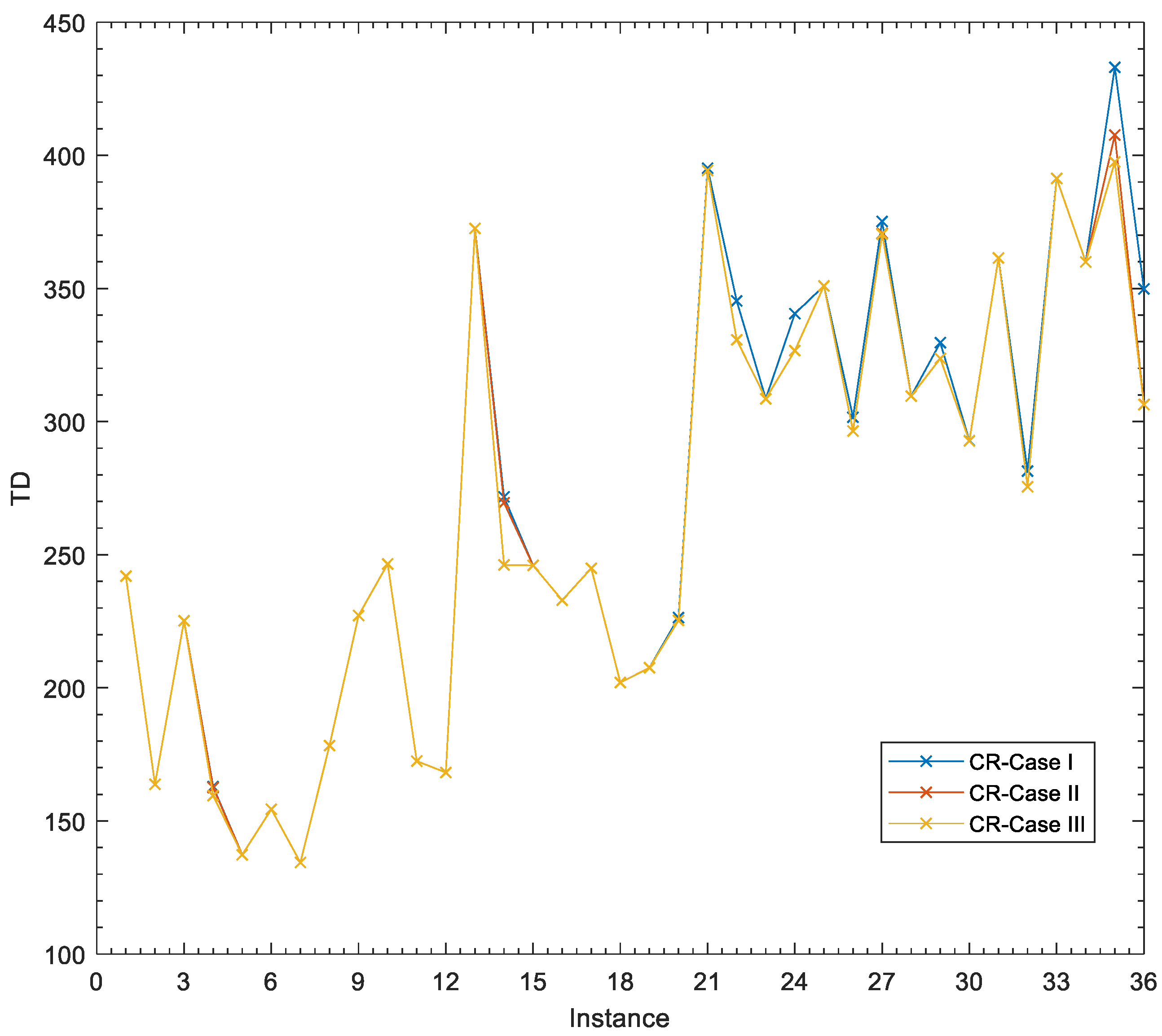
4.3.3. The Sensitivity Analysis of Budget
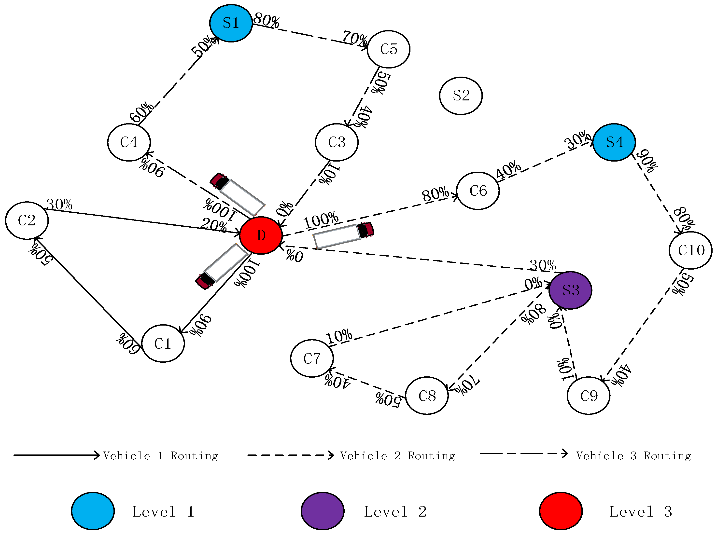
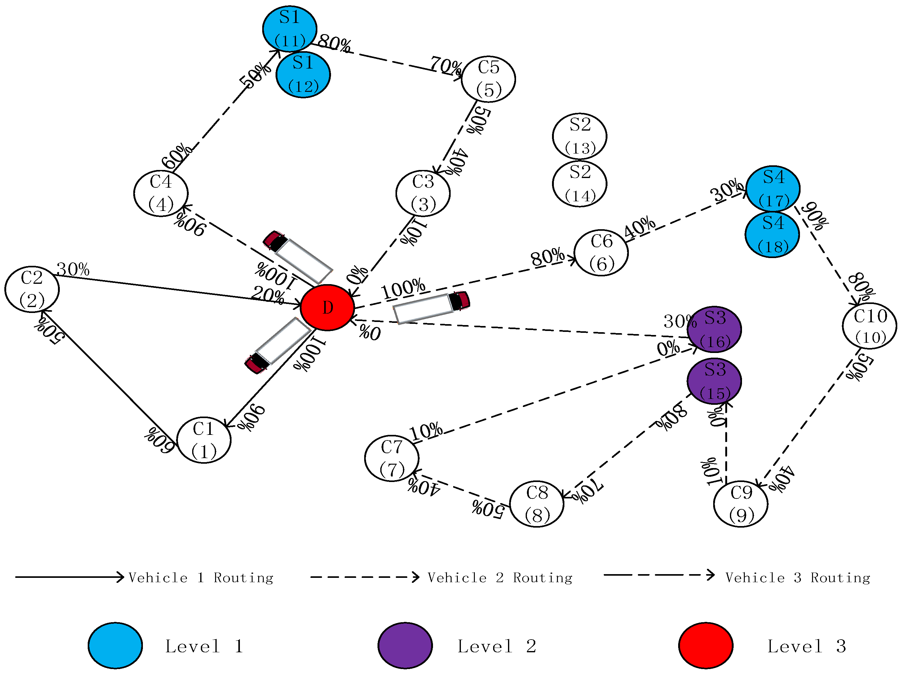
4.3.4. The Sensitivity Analysis of the Number of Corresponding Dummy Nodes of One Candidate Charging Station
5. Conclusions and Discussions
Supplementary Materials
Author Contributions
Funding
Conflicts of Interest
Appendix A


References
- Liu, W.Y.; Lin, C.C.; Chiu, C.R.; Tsao, Y.S.; Wang, Q. Minimizing the Carbon Footprint for the Time-Dependent Heterogeneous-Fleet Vehicle Routing Problem with Alternative Paths. Sustainability 2014, 6, 4658–4684. [Google Scholar] [CrossRef]
- Nie, Y.; Ghamami, M. A corridor-centric approach to planning electric vehicle charging infrastructure. Transp. Res. Part B Methodol. 2013, 57, 172–190. [Google Scholar] [CrossRef]
- Wu, T.; Zeng, B.; He, Y.; Tian, X.; Ou, X. Sustainable Governance for the Opened Electric Vehicle Charging and Upgraded Facilities Market. Sustainability 2017, 9, 2126. [Google Scholar] [CrossRef]
- Yang, J.; Sun, H. Battery swap station location-routing problem with capacitated electric vehicles. Comput. Oper. Res. 2015, 55, 217–232. [Google Scholar] [CrossRef]
- Amini, M.H.; Karabasoglu, O. Optimal Operation of Interdependent Power Systems and Electrified Transportation Networks. Energies 2018, 11, 196. [Google Scholar] [CrossRef]
- Karabasoglu, O.; Michalek, J. Influence of driving patterns on life cycle cost and emissions of hybrid and plug-in electric vehicle powertrains. Energy Policy 2013, 60, 445–461. [Google Scholar] [CrossRef]
- Lajunen, A.; Lipman, T. Lifecycle cost assessment and carbon dioxide emissions of diesel, natural gas, hybrid electric, fuel cell hybrid and electric transit buses. Energy 2016, 106, 329–342. [Google Scholar] [CrossRef]
- Nie, Y.M.; Ghamami, M.; Zockaie, A.; Xiao, F. Optimization of incentive polices for plug-in electric vehicles. Transp. Res. Part B Methodol. 2016, 84, 103–123. [Google Scholar] [CrossRef]
- Viola, F.; Longo, M. On the strategies for the diffusion of EVs: Comparison between Norway and Italy. Int. J. Renew. Energy Res. 2017, 7, 1376–1382. [Google Scholar]
- Lee, C.; Han, J. Benders-and-Price approach for electric vehicle charging station location problem under probabilistic travel range. Transp. Res. Part B Methodol. 2017, 106, 130–152. [Google Scholar] [CrossRef]
- He, F.; Yin, Y.; Zhou, J. Deploying public charging stations for electric vehicles on urban road networks. Transp. Res. Part C Emerg. Technol. 2015, 60, 227–240. [Google Scholar] [CrossRef]
- Morrow, K.; Karner, D.J.F. Plug-in Hybrid Electric Vehicle Charging Infrastructure Review. Report # INL/EXT-08-15058. 2008. Available online: https://www.google.com/url?sa=t&rct=j&q=&esrc=s&source=web&cd=1&cad=rja&uact=8&ved=2ahUKEwjloIOVwuTcAhVKBIgKHacaCZkQFjAAegQIABAC&url=https%3A%2F%2Fwecanfigurethisout.org%2FENERGY%2FLecture_notes%2FElectrification_of_Tranportation_Supporting_Materials%2520%2FINL%2520-%2520PHEV%2520infrastructure%2520review.pdf&usg=AOvVaw3CA9nvecPRE3s554ynb-EY (accessed on 11 August 2018).
- Kuby, M.; Lim, S. The flow-refueling location problem for alternative-fuel vehicles. Socio-Econ. Plan. Sci. 2005, 39, 125–145. [Google Scholar] [CrossRef]
- Melaina, M.; Bremson, J. Refueling availability for alternative fuel vehicle markets: Sufficient urban station coverage. Energy Policy 2008, 36, 3233–3241. [Google Scholar] [CrossRef]
- Romm, J. The car and fuel of the future. Energy Policy 2006, 34, 2609–2614. [Google Scholar] [CrossRef]
- He, F.; Yin, Y.F.; Lawphongpanich, S. Network equilibrium models with battery electric vehicles. Transp. Res. Part B Methodol. 2014, 67, 306–319. [Google Scholar] [CrossRef]
- Huang, S.; He, L.; Gu, Y.; Wood, K.; Benjaafar, S. Design of a mobile charging service for electric vehicles in an urban environment. IEEE Trans. Intell. Transp. Syst. 2015, 16, 787–798. [Google Scholar] [CrossRef]
- Rand, G.K. Methodological choices in depot location studies. Oper. Res. Q. 1976, 27, 241–249. [Google Scholar] [CrossRef]
- Adler, J.D.; Mirchandani, P.B. Online routing and battery reservations for electric vehicles with swappable batteries. Transp. Res. Part B Methodol. 2014, 70, 285–302. [Google Scholar] [CrossRef]
- Hof, J.; Schneider, M.; Goeke, D. Solving the battery swap station location-routing problem with capacitated electric vehicles using an AVNS algorithm for vehicle-routing problems with intermediate stops. Transp. Res. Part B Methodol. 2017, 97, 102–112. [Google Scholar] [CrossRef]
- Mak, H.Y.; Shen, Z.J.M. Infrastructure planning for electric vehicles with battery swapping. Manag. Sci. 2013, 59, 1557–1575. [Google Scholar] [CrossRef]
- Liu, H.; Wang, D.Z.W. Locating multiple types of charging facilities for battery electric vehicles. Transp. Res. Part B Methodol. 2017, 103, 30–55. [Google Scholar] [CrossRef]
- Chen, Z.B.; He, F.; Yin, Y.F. Optimal deployment of charging lanes for electric vehicles in transportation networks. Transp. Res. Part B Methodol. 2016, 91, 344–365. [Google Scholar] [CrossRef]
- Yilmaz, M.; Krein, P.T. Review of battery charger topologies, charging power levels, and infrastructure for plug-in electric and hybrid vehicles. IEEE Trans. Power Electron. 2013, 28, 2151–2169. [Google Scholar] [CrossRef]
- Nagy, G.; Salhi, S. Location-routing: Issues, models and methods. Eur. J. Oper. Res. 2006, 177, 649–672. [Google Scholar] [CrossRef]
- Watson-Gandy, C.D.T.; Dohrn, P.J. Depot location with van salesmen—A practical approach. Omega 1973, 1, 321–329. [Google Scholar] [CrossRef]
- Caballero, R.; Gonzalez, M.; Guerrero, F.M.; Molina, J.; Paralera, C. Solving a multiobjective location routing problem with a metaheuristic based on tabu search: Application to a real case in Andalusia. Eur. J. Oper. Res. 2007, 177, 1751–1763. [Google Scholar] [CrossRef]
- Murty, K.G.; Djang, P.A. The U.S. army national guard’s mobile training simulators location and routing problem. Oper. Res. 1999, 47, 175–182. [Google Scholar] [CrossRef]
- Lin, C.K.Y.; Chow, C.K.; Chen, A. A location-routing loading problem for bill delivery services. Comput. Ind. Eng. 2002, 43, 5–25. [Google Scholar] [CrossRef]
- Lee, Y.; Kim, S.i.; Lee, S.; Kang, K. A location-routing problem in designing optical internet access with WDM systems. Photonic Netw. Commun. 2003, 6, 151–160. [Google Scholar] [CrossRef]
- An, Y.; Zeng, B.; Zhang, Y.; Zhao, L. Reliable p-median facility location problem: Two-stage robust models and algorithms. Transp. Res. Part B Methodol. 2014, 64, 54–72. [Google Scholar] [CrossRef]
- Campbell, J.F. Hub location and the p-hub median problem. Oper. Res. 1996, 44, 923–935. [Google Scholar] [CrossRef]
- Frade, I.; Ribeiro, A.; Gonçalves, G.; Antunes, A. Optimal location of charging stations for electric vehicles in a neighborhood in lisbon, portugal. Transp. Res. Rec. 2011, 2252, 91–98. [Google Scholar] [CrossRef]
- Chung, S.H.; Kwon, C. Multi-period planning for electric car charging station locations: A case of Korean expressways. Eur. J. Oper. Res. 2015, 242, 677–687. [Google Scholar] [CrossRef]
- Kuby, M.; Lines, L.; Schultz, R.; Xie, Z.; Kim, J.G.; Lim, S. Optimization of hydrogen stations in Florida using the flow-refueling location model. Int. J. Hydrog. Energy 2009, 34, 6045–6064. [Google Scholar] [CrossRef]
- Wang, Y.W.; Lin, C.C. Locating multiple types of recharging stations for battery-powered electric vehicle transport. Transp. Res. Part E Logist. Transp. Rev. 2013, 58, 76–87. [Google Scholar] [CrossRef]
- Gendreau, M.; Tarantilis, C.D. Solving Large-Scale Vehicle Routing Problems with Time Windows: The State-of-the-Art. Technical Report 2010-04, CIRRELT, Montréal. Available online: https://www.cirrelt.ca/Documents.Travail/CIRRELT-2010-04.pdf (accessed on 11 August 2018).
- Bodin, L.; Golden, B.; Assad, A.; Ball, M. Routing and scheduling of vehicles and crews: The state of the art. Comput. Oper. Res. 1983, 10, 62–212. [Google Scholar]
- Schragf, L. Formulation and structure of more complex/realistic routing and scheduling problems. Networks 1981, 11, 229–232. [Google Scholar] [CrossRef]
- Rod, M.; Ashill, N.J.; Gibbs, T. Customer perceptions of frontline employee service delivery: A study of Russian bank customer satisfaction and behavioral intentions. J. Retail. Consum. Serv. 2016, 30, 212–221. [Google Scholar] [CrossRef]
- Blanutsa, V.I. The postal-geographical location: The notion and measurement algorithm (exemplified by the postal network of Siberia in the early 20th century). Geogr. Nat. Resour. 2010, 31, 308–316. [Google Scholar] [CrossRef]
- Sun, L.; Zhao, L.; Hou, J. Optimization of postal express line network under mixed driving pattern of trucks. Transp. Res. Part E Logist. Transp. Rev. 2015, 77, 147–169. [Google Scholar] [CrossRef]
- Caceres, H.; Batta, R.; He, Q. Special Need Students School Bus Routing: Consideration for Mixed Load and Heterogeneous Fleet. Socio-Economic Planning Sciences. Available online: https://www.sciencedirect.com/science/article/pii/S0038012117301374 (accessed on 11 August 2018).
- Mokhtari, N.A.; Ghezavati, V. Integration of efficient multi-objective ant-colony and a heuristic method to solve a novel multi-objective mixed load school bus routing model. Appl. Soft Comput. 2018, 68, 92–109. [Google Scholar] [CrossRef]
- Section, T.; Bodin, L. Optimizing single vehicle many-to-many operations with desired delivery times: I. Scheduling. Transp. Sci. 1985, 19, 378–410. [Google Scholar]
- Section, T.; Bodin, L. Optimizing single vehicle many-to-many operations with desired delivery times: II. Routing. Transp. Sci. 1985, 19, 411–435. [Google Scholar]
- Schneider, M.; Stenger, A.; Goeke, D. The electric vehicle-routing problem with time windows and recharging stations. Transp. Sci. 2014, 48, 500–520. [Google Scholar] [CrossRef]
- Keskin, M.; Çatay, B. Partial recharge strategies for the electric vehicle routing problem with time windows. Transp. Res. Part C Emerg. Technol. 2016, 65, 111–127. [Google Scholar] [CrossRef]
- Yarow, J. The Cost of a Better Place Battery Swapping Station: $500,000. 2009. Available online: http://www.businessinsider.com/the-cost-of-a-better-place-battery-swapping-station-500000-2009-4 (accessed on 11 August 2018).
- Marra, F.; Yang, G.Y.; Traholt, C.; Larsen, E.; Rasmussen, C.N.; Shi, Y. Demand profile study of battery electric vehicle under different charging options. In Proceedings of the IEEE Power and Energy Social General Meeting, San Diego, CA, USA, 22–26 July 2012. [Google Scholar]
- Neubauer, J.; Wood, E.; Pesaran, A. Project Milestone. Analysis of Range Extension Techniques for Battery Electric Vehicles; Technical Report; National Renewable Energy Laboratory (NREL): Golden, CO, USA, 2013.
- Straubel, J. Driving Range for the Model S Family. Tesla Motors. 2015. Available online: https://www.tesla.com/blog/driving-range-model-s-family (accessed on 11 August 2018).
- Sherali, H.D.; Adams, W.P. A Reformulation-Linearization Technique for Solving Discrete and Continuous Nonconvex Problems; Kluwer Academic Publishers: Dordrecht, The Netherlands, 1999. [Google Scholar]


| Indices | Definition |
|---|---|
| Index of depot instances and every route starts at and ends at | |
| Index of nodes, | |
| Index of physical link between two adjacent nodes, | |
| Sets | |
| Set of feasible types of plug-in charging station; , where , , refer to the level , , and charging station, respectively | |
| Set of recharging station | |
| Set of dummy vertices of | |
| Set of dummy vertices of depot instance | |
| Set of recharging visits including depot instance | |
| Set of customers | |
| Set of customers including depot instance | |
| Set of customer vertices including visits to recharging stations, | |
| Set of customers and recharging visits including depot instance , | |
| Set of customers and recharging visits including depot instance , | |
| Set of customers and recharging visits including depot instance and , | |
| Parameters | |
| The type plug in charging station | |
| The budget limit for building charging station | |
| Capacity of mobile charging vehicles | |
| Distance of link | |
| Travel time of link | |
| Recharging rate of type | |
| Cost of building a plug-in charging station of type | |
| The power demand for one electric car in node | |
| Battery capacity for mobile charging service car | |
| Charge consumption rate in traveling | |
| The number of corresponding dummy nodes of one candidate charging station | |
| Demand number of node , and if not belong to set V | |
| Earliest start of service at node | |
| Latest start of service at node , it is always a positive number of infinity | |
| Service time at node | |
| The sufficiently large constant | |
| Variables | |
| =1, if a charging station of type should be built in node ; otherwise = 0 | |
| The time of arrive at node | |
| The recharging amount of electricity at node | |
| if arc is traveled; otherwise | |
| The remaining battery on arrival at node |
| No. | Instance | #v | TD | R_A | ϕ = 1 | ϕ = 2 | ϕ = 3 |
|---|---|---|---|---|---|---|---|
| 1 | C101–5 | 3 | 241.97 | 267.98 | 0 | 1 | 1 |
| 2 | C103–5 | 2 | 163.77 | 34.83 | 1 | 0 | 0 |
| 3 | C206–5 | 2 | 225.21 | 231.58 | 0 | 1 | 2 |
| 4 | C208–5 | 1 | 162.89 | 282.06 | 1 | 1 | 0 |
| 5 | R104–5 | 2 | 137.32 | 156.88 | 1 | 0 | 0 |
| 6 | R105–5 | 2 | 154.4 | 105.74 | 1 | 0 | 0 |
| 7 | R202–5 | 1 | 134.41 | 194.35 | 2 | 0 | 0 |
| 8 | R203–5 | 1 | 178.31 | 153.76 | 1 | 1 | 1 |
| 9 | RC105–5 | 2 | 227.19 | 0 | 0 | 0 | 0 |
| 10 | RC108–5 | 2 | 246.54 | 62.94 | 1 | 0 | 0 |
| 11 | RC204–5 | 1 | 172.49 | 169.06 | 1 | 0 | 0 |
| 12 | RC208–5 | 1 | 168.21 | 153.85 | 1 | 0 | 1 |
| 13 | C101–10 | 3 | 372.55 | 283.8 | 1 | 0 | 3 |
| 14 | C104–10 | 2 | 271.72 | 249.76 | 1 | 1 | 1 |
| 15 | C202–10 | 2 | 245.98 | 274.51 | 0 | 1 | 1 |
| 16 | C205–10 | 2 | 232.92 | 410.85 | 1 | 1 | 2 |
| 17 | R102–10 | 3 | 244.9 | 98.28 | 2 | 0 | 0 |
| 18 | R103–10 | 3 | 202.01 | 116.7 | 2 | 0 | 0 |
| 19 | R201–10 | 3 | 207.53 | 294.24 | 2 | 0 | 0 |
| 20 | R203–10 | 1 | 226.4 | 289.04 | 1 | 1 | 2 |
| 21 | RC102–10 | 3 | 395.18 | 141.88 | 2 | 0 | 0 |
| 22 | RC108–10 | 3 | 345.35 | 189.61 | 1 | 1 | 0 |
| 23 | RC201–10 | 2 | 308.59 | 271.78 | 1 | 1 | 1 |
| 24 | RC205–10 | 3 | 340.51 | 301.86 | 0 | 3 | 0 |
| 25 | C103–15 | 3 | 350.99 | 414.78 | 1 | 1 | 2 |
| 26 | C106–15 | 4 | 301.64 | 229.71 | 1 | 1 | 2 |
| 27 | C202–15 | 3 | 375.19 | 575.1 | 1 | 0 | 4 |
| 28 | C208–15 | 2 | 309.62 | 380.09 | 0 | 1 | 3 |
| 29 | R102–15 | 4 | 329.64 | 107.43 | 2 | 0 | 0 |
| 30 | R105–15 | 3 | 292.81 | 216.15 | 2 | 0 | 0 |
| 31 | R202–15 | 3 | 361.47 | 477.85 | 0 | 2 | 2 |
| 32 | R209–15 | 2 | 281.41 | 353.83 | 1 | 1 | 2 |
| 33 | RC103–15 | 4 | 391.34 | 74.01 | 2 | 0 | 0 |
| 34 | RC108–15 | 3 | 359.98 | 269.52 | 2 | 0 | 0 |
| 35 | RC202–15 | 4 | 433.09 | 228.75 | 1 | 1 | 2 |
| 36 | RC204–15 | 2 | 349.82 | 410.29 | 1 | 1 | 2 |
| No. | Instance | Seven | Nine | Δv(%) | ΔTD(%) | ||||
|---|---|---|---|---|---|---|---|---|---|
| #v | TD | R_A | #v | TD | R_A | ||||
| 1 | C101–5 | 3 | 241.97 | 267.98 | 3 | 234.72 | 127.25 | 0.00 | 3.00 |
| 2 | C103–5 | 2 | 163.77 | 34.83 | 2 | 161.26 | 0 | 0.00 | 1.53 |
| 3 | C206–5 | 2 | 225.21 | 231.58 | 2 | 219.54 | 47.46 | 0.00 | 2.52 |
| 4 | C208–5 | 1 | 162.89 | 282.06 | 1 | 157.72 | 87.76 | 0.00 | 3.17 |
| 5 | R104–5 | 2 | 137.32 | 156.88 | 2 | 136.45 | 22.72 | 0.00 | 0.63 |
| 6 | R105–5 | 2 | 154.40 | 105.74 | 2 | 151.15 | 0 | 0.00 | 2.10 |
| 7 | R202–5 | 1 | 134.41 | 194.35 | 1 | 126.83 | 80.17 | 0.00 | 5.64 |
| 8 | R203–5 | 1 | 178.31 | 153.76 | 1 | 178.17 | 118.25 | 0.00 | 0.08 |
| 9 | RC105–5 | 2 | 227.19 | 0 | 2 | 227.19 | 0 | 0.00 | 0.02 |
| 10 | RC108–5 | 2 | 246.54 | 62.94 | 2 | 245.87 | 0 | 0.00 | 0.27 |
| 11 | RC204–5 | 1 | 172.49 | 169.06 | 1 | 172.49 | 69.37 | 0.00 | 0.00 |
| 12 | RC208–5 | 1 | 168.21 | 153.85 | 1 | 163.33 | 108.21 | 0.00 | 2.90 |
| 13 | C101–10 | 3 | 372.55 | 283.80 | 3 | 366.5 | 218.68 | 0.00 | 1.62 |
| 14 | C104–10 | 2 | 271.72 | 249.76 | 2 | 261.21 | 151 | 0.00 | 3.87 |
| 15 | C202–10 | 2 | 245.98 | 274.51 | 2 | 243.19 | 266.12 | 0.00 | 1.13 |
| 16 | C205–10 | 2 | 232.92 | 410.85 | 2 | 228.32 | 172.51 | 0.00 | 1.97 |
| 17 | R102–10 | 3 | 244.90 | 98.28 | 3 | 242.42 | 47.44 | 0.00 | 1.01 |
| 18 | R103–10 | 3 | 202.01 | 116.70 | 3 | 193.69 | 0 | 0.00 | 4.12 |
| 19 | R201–10 | 3 | 207.53 | 294.24 | 3 | 206.05 | 59.69 | 0.00 | 0.71 |
| 20 | R203–10 | 1 | 226.40 | 289.04 | 1 | 214.61 | 261.43 | 0.00 | 5.21 |
| 21 | RC102–10 | 3 | 395.18 | 141.88 | 3 | 385.79 | 0 | 0.00 | 2.38 |
| 22 | RC108–10 | 3 | 345.35 | 189.61 | 3 | 331.14 | 80.33 | 0.00 | 4.11 |
| 23 | RC201–10 | 2 | 308.59 | 271.78 | 2 | 304.00 | 0 | 0.00 | 1.49 |
| 24 | RC205–10 | 3 | 340.51 | 301.86 | 2 | 325.27 | 195.29 | 33.33 | 4.48 |
| 25 | C103–15 | 3 | 350.99 | 414.78 | 3 | 343.47 | 399.38 | 0.00 | 2.14 |
| 26 | C106–15 | 4 | 301.64 | 229.71 | 3 | 267.82 | 103.17 | 25.00 | 11.21 |
| 27 | C202–15 | 3 | 375.19 | 575.10 | 2 | 362.59 | 359.57 | 33.33 | 3.36 |
| 28 | C208–15 | 2 | 309.62 | 380.09 | 2 | 305.90 | 286.04 | 0.00 | 1.20 |
| 29 | R102–15 | 4 | 329.64 | 107.43 | 4 | 326.01 | 98.50 | 0.00 | 1.10 |
| 30 | R105–15 | 3 | 292.81 | 216.15 | 3 | 290.12 | 98.80 | 0.00 | 0.92 |
| 31 | R202–15 | 3 | 361.47 | 477.85 | 3 | 358.28 | 340.91 | 0.00 | 0.88 |
| 32 | R209–15 | 2 | 281.41 | 353.83 | 2 | 272.14 | 247.60 | 0.00 | 3.29 |
| 33 | RC103–15 | 4 | 391.34 | 74.01 | 4 | 389.89 | 32.89 | 0.00 | 0.37 |
| 34 | RC108–15 | 3 | 359.98 | 269.52 | 3 | 358.86 | 56.47 | 0.00 | 0.31 |
| 35 | RC202–15 | 4 | 433.09 | 228.75 | 3 | 398.76 | 208.77 | 25.00 | 7.93 |
| 36 | RC204–15 | 2 | 349.82 | 410.29 | 2 | 306.37 | 256.65 | 0.00 | 12.42 |
| Average | 2.42 | 270.65 | 235.36 | 2.31 | 262.70 | 127.85 | 3.24 | 2.75 | |
| No. | Instance | CR–Case I | CR–Case II | CR–Case III | ||||||
|---|---|---|---|---|---|---|---|---|---|---|
| #v | TD | R_A | #v | TD | R_A | #v | TD | R_A | ||
| 1 | C101–5 | 3 | 241.97 | 267.98 | 3 | 241.97 | 267.98 | 3 | 241.97 | 267.98 |
| 2 | C103–5 | 2 | 163.77 | 34.83 | 2 | 163.77 | 34.83 | 2 | 163.77 | 34.83 |
| 3 | C206–5 | 2 | 225.21 | 231.58 | 2 | 225.21 | 231.58 | 2 | 225.21 | 231.58 |
| 4 | C208–5 | 1 | 162.89 | 282.06 | 1 | 162.60 | 224.68 | 1 | 159.53 | 119.62 |
| 5 | R104–5 | 2 | 137.32 | 156.88 | 2 | 137.32 | 156.88 | 2 | 137.32 | 156.88 |
| 6 | R105–5 | 2 | 154.4 | 105.74 | 2 | 154.4 | 105.74 | 2 | 154.4 | 105.74 |
| 7 | R202–5 | 1 | 134.41 | 194.35 | 1 | 134.41 | 194.35 | 1 | 134.41 | 194.35 |
| 8 | R203–5 | 1 | 178.31 | 153.76 | 1 | 178.31 | 153.76 | 1 | 178.31 | 153.76 |
| 9 | RC105–5 | 2 | 227.19 | 0 | 2 | 227.19 | 0 | 2 | 227.19 | 0 |
| 10 | RC108–5 | 2 | 246.54 | 62.94 | 2 | 246.54 | 62.94 | 2 | 246.54 | 62.94 |
| 11 | RC204–5 | 1 | 172.49 | 169.06 | 1 | 172.49 | 169.06 | 1 | 172.49 | 169.06 |
| 12 | RC208–5 | 1 | 168.21 | 153.85 | 1 | 168.21 | 153.85 | 1 | 168.21 | 153.85 |
| 13 | C101–10 | 3 | 372.55 | 283.8 | 3 | 372.55 | 283.8 | 3 | 372.55 | 283.8 |
| 14 | C104–10 | 2 | 271.72 | 249.76 | 2 | 269.53 | 310.39 | 1 | 246.17 | 431.35 |
| 15 | C202–10 | 2 | 245.98 | 274.51 | 2 | 245.98 | 274.51 | 2 | 245.98 | 274.51 |
| 16 | C205–10 | 2 | 232.92 | 410.85 | 2 | 232.92 | 410.85 | 2 | 232.92 | 410.85 |
| 17 | R102–10 | 3 | 244.9 | 98.28 | 3 | 244.9 | 98.28 | 3 | 244.9 | 98.28 |
| 18 | R103–10 | 3 | 202.01 | 116.7 | 3 | 202.01 | 116.7 | 3 | 202.01 | 116.7 |
| 19 | R201–10 | 3 | 207.53 | 294.24 | 3 | 207.53 | 294.24 | 3 | 207.53 | 294.24 |
| 20 | R203–10 | 1 | 226.4 | 289.04 | 1 | 225.35 | 287.98 | 1 | 225.35 | 287.98 |
| 21 | RC102–10 | 3 | 395.18 | 141.88 | 3 | 394.34 | 95.66 | 3 | 394.34 | 95.66 |
| 22 | RC108–10 | 3 | 345.35 | 189.61 | 2 | 330.72 | 239.73 | 2 | 330.72 | 239.73 |
| 23 | RC201–10 | 2 | 308.59 | 271.78 | 2 | 308.59 | 271.78 | 2 | 308.59 | 271.78 |
| 24 | RC205–10 | 3 | 340.51 | 301.86 | 2 | 326.67 | 303.52 | 2 | 326.67 | 303.52 |
| 25 | C103–15 | 3 | 350.99 | 414.78 | 3 | 350.99 | 414.78 | 3 | 350.99 | 414.78 |
| 26 | C106–15 | 4 | 301.64 | 229.71 | 3 | 296.45 | 381.75 | 3 | 296.45 | 381.75 |
| 27 | C202–15 | 3 | 375.19 | 575.1 | 2 | 370.69 | 531.94 | 2 | 370.44 | 557.37 |
| 28 | C208–15 | 2 | 309.62 | 380.09 | 2 | 309.62 | 380.09 | 2 | 309.62 | 380.09 |
| 29 | R102–15 | 4 | 329.64 | 107.43 | 4 | 323.71 | 162.38 | 4 | 323.71 | 162.38 |
| 30 | R105–15 | 3 | 292.81 | 216.15 | 3 | 292.73 | 238.02 | 3 | 292.73 | 238.02 |
| 31 | R202–15 | 3 | 361.47 | 477.85 | 3 | 361.47 | 477.85 | 3 | 361.47 | 477.85 |
| 32 | R209–15 | 2 | 281.41 | 353.83 | 2 | 275.56 | 457.28 | 2 | 275.56 | 457.28 |
| 33 | RC103–15 | 4 | 391.34 | 74.01 | 4 | 391.34 | 74.01 | 4 | 391.34 | 74.01 |
| 34 | RC108–15 | 3 | 359.98 | 269.52 | 3 | 359.98 | 269.52 | 3 | 359.98 | 269.52 |
| 35 | RC202–15 | 4 | 433.09 | 228.75 | 3 | 407.65 | 386.68 | 2 | 397.56 | 695.98 |
| 36 | RC204–15 | 2 | 349.82 | 410.29 | 2 | 306.44 | 424.81 | 2 | 306.40 | 421.71 |
| Average | 2.42 | 270.65 | 235.36 | 2.28 | 267.23 | 248.39 | 2.22 | 266.21 | 258.05 | |
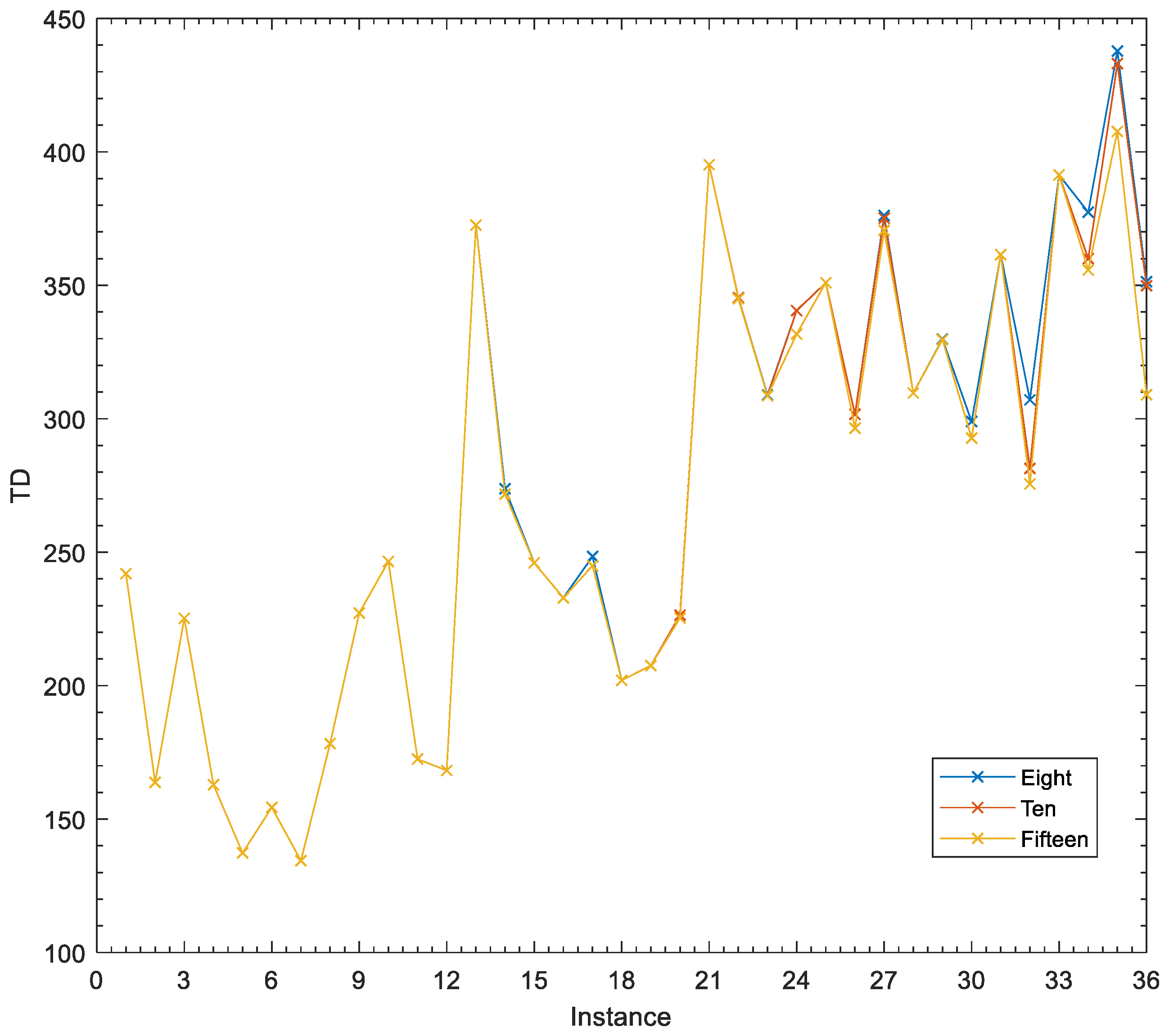
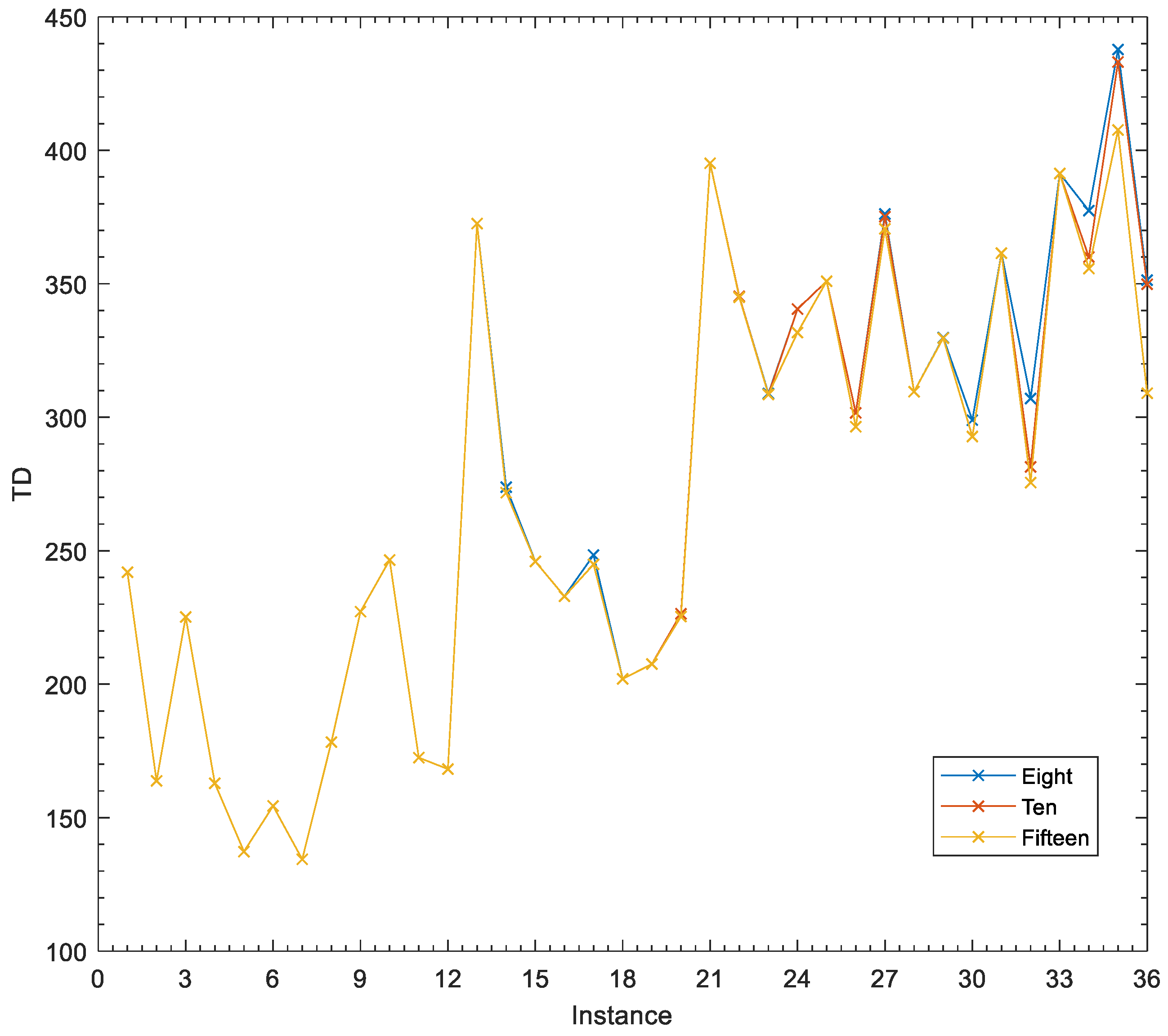
| No. | Instance | Eight | Ten | Fifteen | ||||||
|---|---|---|---|---|---|---|---|---|---|---|
| #v | TD | R_A | #v | TD | R_A | #v | TD | R_A | ||
| 1 | C101–5 | 3 | 241.97 | 267.98 | 3 | 241.97 | 267.98 | 3 | 241.97 | 267.98 |
| 2 | C103–5 | 2 | 163.77 | 34.83 | 2 | 163.77 | 34.83 | 2 | 163.77 | 34.83 |
| 3 | C206–5 | 2 | 225.21 | 231.58 | 2 | 225.21 | 231.58 | 2 | 225.21 | 231.58 |
| 4 | C208–5 | 1 | 162.89 | 282.06 | 1 | 162.89 | 282.06 | 1 | 162.89 | 282.06 |
| 5 | 104–5 | 2 | 137.32 | 156.88 | 2 | 137.32 | 156.88 | 2 | 137.32 | 156.88 |
| 6 | R105–5 | 2 | 154.4 | 105.74 | 2 | 154.4 | 105.74 | 2 | 154.4 | 105.74 |
| 7 | R202–5 | 1 | 134.41 | 194.35 | 1 | 134.41 | 194.35 | 1 | 134.41 | 194.35 |
| 8 | R203–5 | 1 | 178.31 | 153.76 | 1 | 178.31 | 153.76 | 1 | 178.31 | 153.76 |
| 9 | RC105–5 | 2 | 227.19 | 0 | 2 | 227.19 | 0 | 2 | 227.19 | 0 |
| 10 | RC108–5 | 2 | 246.54 | 62.94 | 2 | 246.54 | 62.94 | 2 | 246.54 | 62.94 |
| 11 | RC204–5 | 1 | 172.49 | 169.06 | 1 | 172.49 | 169.06 | 1 | 172.49 | 169.06 |
| 12 | RC208–5 | 1 | 168.21 | 153.85 | 1 | 168.21 | 153.85 | 1 | 168.21 | 153.85 |
| 13 | C101–10 | 3 | 372.55 | 283.8 | 3 | 372.55 | 283.8 | 3 | 372.55 | 283.8 |
| 14 | C104–10 | 2 | 273.80 | 266.84 | 2 | 271.72 | 249.76 | 2 | 271.72 | 249.76 |
| 15 | C202–10 | 2 | 245.98 | 274.51 | 2 | 245.98 | 274.51 | 2 | 245.98 | 274.51 |
| 16 | C205–10 | 2 | 232.92 | 410.85 | 2 | 232.92 | 410.85 | 2 | 232.92 | 410.85 |
| 17 | R102–10 | 3 | 248.38 | 213.45 | 3 | 244.9 | 98.28 | 3 | 244.9 | 98.28 |
| 18 | R103–10 | 3 | 202.01 | 116.7 | 3 | 202.01 | 116.7 | 3 | 202.01 | 116.7 |
| 19 | R201–10 | 3 | 207.53 | 294.24 | 3 | 207.53 | 294.24 | 3 | 207.53 | 294.24 |
| 20 | R203–10 | 1 | 226.4 | 289.04 | 1 | 226.4 | 289.04 | 1 | 225.35 | 287.99 |
| 21 | RC102–10 | 3 | 395.18 | 141.88 | 3 | 395.18 | 141.88 | 3 | 395.18 | 141.88 |
| 22 | RC108–10 | 3 | 345.35 | 189.61 | 3 | 345.35 | 189.61 | 3 | 344.98 | 271.91 |
| 23 | RC201–10 | 2 | 308.90 | 253.10 | 2 | 308.59 | 271.78 | 2 | 308.59 | 271.78 |
| 24 | RC205–10 | 3 | 340.51 | 301.86 | 3 | 340.51 | 301.86 | 2 | 331.74 | 360.18 |
| 25 | C103–15 | 3 | 350.99 | 414.78 | 3 | 350.99 | 414.78 | 3 | 350.99 | 414.78 |
| 26 | C106–15 | 4 | 301.64 | 229.71 | 4 | 301.64 | 229.71 | 3 | 296.45 | 324.68 |
| 27 | C202–15 | 3 | 376.16 | 384.22 | 3 | 375.19 | 575.1 | 2 | 370.58 | 415.04 |
| 28 | C208–15 | 2 | 309.62 | 380.09 | 2 | 309.62 | 380.09 | 2 | 309.62 | 380.09 |
| 29 | R102–15 | 4 | 329.84 | 176.28 | 4 | 329.64 | 107.43 | 4 | 329.64 | 107.43 |
| 30 | R105–15 | 3 | 298.93 | 114.18 | 3 | 292.81 | 216.15 | 3 | 292.75 | 219.09 |
| 31 | R202–15 | 3 | 361.47 | 477.85 | 3 | 361.47 | 477.85 | 3 | 361.47 | 477.85 |
| 32 | R209–15 | 3 | 307.07 | 245.63 | 2 | 281.41 | 353.83 | 2 | 275.56 | 397.65 |
| 33 | RC103–15 | 4 | 391.34 | 74.01 | 4 | 391.34 | 74.01 | 4 | 391.34 | 74.01 |
| 34 | RC108–15 | 3 | 377.38 | 161.32 | 3 | 359.98 | 269.52 | 3 | 355.73 | 324.76 |
| 35 | RC202–15 | 4 | 437.77 | 326.54 | 4 | 433.09 | 228.75 | 3 | 407.65 | 372.54 |
| 36 | RC204–15 | 3 | 351.35 | 315.94 | 2 | 349.82 | 410.29 | 2 | 308.99 | 367.56 |
| Average | 2.47 | 272.38 | 226.37 | 2.42 | 270.65 | 235.36 | 2.31 | 267.97 | 243.07 | |
| No. | Instance | Seven | Nine | Δv(%) | ΔTD(%) | ||||
|---|---|---|---|---|---|---|---|---|---|
| #v | TD | R_A | #v | TD | R_A | ||||
| 1 | C101–5 | 3 | 241.97 | 267.98 | 3 | 234.72 | 127.25 | 0 | 3 |
| 2 | C103–5 | 2 | 163.77 | 34.83 | 2 | 161.26 | 0 | 0 | 1.53 |
| 3 | C206–5 | 2 | 225.21 | 231.58 | 2 | 219.54 | 47.46 | 0 | 2.52 |
| 4 | C208–5 | 1 | 162.26 | 138.38 | 1 | 157.72 | 87. 76 | 0 | 2.8 |
| 5 | R104–5 | 2 | 137.32 | 156.88 | 2 | 136.45 | 22.72 | 0 | 0.63 |
| 6 | R105–5 | 2 | 154.4 | 105.74 | 2 | 151.15 | 0 | 0 | 2.1 |
| 7 | R202–5 | 1 | 134.41 | 194.35 | 1 | 126.83 | 80.17 | 0 | 5.64 |
| 8 | R203–5 | 1 | 178.31 | 153.76 | 1 | 178.17 | 118.25 | 0 | 0.08 |
| 9 | RC105–5 | 2 | 227.19 | 0 | 2 | 227.19 | 0 | 0 | 0 |
| 10 | RC108–5 | 2 | 246.54 | 62.94 | 2 | 245.87 | 0 | 0 | 0.27 |
| 11 | RC204–5 | 1 | 172.49 | 169.06 | 1 | 172.49 | 69.37 | 0 | 0 |
| 12 | RC208–5 | 1 | 168.21 | 153.85 | 1 | 163.33 | 108.21 | 0 | 2.9 |
| 13 | C101–10 | 3 | 372.55 | 283.8 | 3 | 366.5 | 218.68 | 0 | 1.62 |
| 14 | C104–10 | 2 | 271.72 | 249.76 | 2 | 261.21 | 151 | 0 | 3.87 |
| 15 | C202–10 | 2 | 245.98 | 274.51 | 2 | 243.19 | 266.12 | 0 | 1.13 |
| 16 | C205–10 | 2 | 232.92 | 410.85 | 2 | 228.32 | 172.51 | 0 | 1.97 |
| 17 | R102–10 | 3 | 244.9 | 98.28 | 3 | 242.42 | 47.44 | 0 | 1.01 |
| 18 | R103–10 | 3 | 202.01 | 116.7 | 3 | 193.69 | 0 | 0 | 4.12 |
| 19 | R201–10 | 3 | 207.53 | 294.24 | 3 | 206.05 | 59.69 | 0 | 0.71 |
| 20 | R203–10 | 1 | 224.71 | 287.35 | 1 | 214.62 | 261.43 | 0 | 4.49 |
| 21 | RC102–10 | 3 | 395.18 | 141.88 | 3 | 385.79 | 0 | 0 | 2.38 |
| 22 | RC108–10 | 3 | 345.35 | 189.61 | 3 | 331.14 | 80.33 | 0 | 4.11 |
| 23 | RC201–10 | 2 | 308.59 | 271.78 | 2 | 304 | 0 | 0 | 1.49 |
| 24 | RC205–10 | 3 | 340.51 | 301.86 | 2 | 325.27 | 195.29 | 33.33 | 4.48 |
| 25 | C103–15 | 3 | 350.99 | 414.78 | 3 | 343.47 | 399.38 | 0 | 2.14 |
| 26 | C106–15 | 3 | 283.24 | 293.87 | 3 | 267.82 | 103.17 | 0 | 5.44 |
| 27 | C202–15 | 3 | 375.19 | 575.1 | 2 | 362.59 | 359.57 | 33.33 | 3.36 |
| 28 | C208–15 | 2 | 309.48 | 519.20 | 2 | 305.90 | 286.04 | 0 | 1.16 |
| 29 | R102–15 | 4 | 329.64 | 107.43 | 4 | 326.01 | 98.5 | 0 | 1.1 |
| 30 | R105–15 | 3 | 292.81 | 216.15 | 3 | 290.12 | 98.8 | 0 | 0.92 |
| 31 | R202–15 | 3 | 361.47 | 477.85 | 3 | 358.28 | 340.91 | 0 | 0.88 |
| 32 | R209–15 | 2 | 281.41 | 353.83 | 2 | 272.14 | 247.6 | 0 | 3.29 |
| 33 | RC103–15 | 4 | 391.34 | 74.01 | 4 | 389.89 | 32.89 | 0 | 0.37 |
| 34 | RC108–15 | 3 | 359.98 | 269.52 | 3 | 358.86 | 56.47 | 0 | 0.31 |
| 35 | RC202–15 | 3 | 419.07 | 386.99 | 3 | 398.76 | 208.77 | 0 | 4.85 |
| 36 | RC204–15 | 2 | 309.69 | 359.98 | 2 | 306.37 | 256.65 | 0 | 1.07 |
| Average | 2.36 | 268.57 | 239.96 | 2.31 | 262.7 | 127.85 | 1.85 | 2.16 | |
© 2018 by the authors. Licensee MDPI, Basel, Switzerland. This article is an open access article distributed under the terms and conditions of the Creative Commons Attribution (CC BY) license (http://creativecommons.org/licenses/by/4.0/).
Share and Cite
Cui, S.; Zhao, H.; Zhang, C. Multiple Types of Plug-In Charging Facilities’ Location-Routing Problem with Time Windows for Mobile Charging Vehicles. Sustainability 2018, 10, 2855. https://doi.org/10.3390/su10082855
Cui S, Zhao H, Zhang C. Multiple Types of Plug-In Charging Facilities’ Location-Routing Problem with Time Windows for Mobile Charging Vehicles. Sustainability. 2018; 10(8):2855. https://doi.org/10.3390/su10082855
Chicago/Turabian StyleCui, Shaohua, Hui Zhao, and Cuiping Zhang. 2018. "Multiple Types of Plug-In Charging Facilities’ Location-Routing Problem with Time Windows for Mobile Charging Vehicles" Sustainability 10, no. 8: 2855. https://doi.org/10.3390/su10082855
APA StyleCui, S., Zhao, H., & Zhang, C. (2018). Multiple Types of Plug-In Charging Facilities’ Location-Routing Problem with Time Windows for Mobile Charging Vehicles. Sustainability, 10(8), 2855. https://doi.org/10.3390/su10082855