Energy and Ecological Sustainability: Challenges and Panoramas in Belt and Road Initiative Countries

Abstract

Innovation and globalization fosters a tendency towards multiparty collaboration and strategic contacts among nations. A similar path was followed by the Chinese administration in 2013, with its “Belt and Road Initiative” (BRI). The most important objective of the present fact-finding study was to demonstrate the links between economic growth, energy consumption, urbanization, gross fixed capital formation, trade openness, financial development and carbon emissions (ecological degradation) from a panel of 47 BRI economies, over a time span of 1980 to 2016. Dynamic panel estimations (dynamic ordinary least square (DOLS) and fully modified ordinary least square (FMOLS)) were engaged to examine the long-run links between the subjected variables. Synchronized outcomes for the full panel show that energy consumption, gross fixed capital formation, economic growth, financial development, and urbanization unfavorably led to environmental degradation (CO₂ emissions). However, trade openness is negatively correlated with emissions. Furthermore, pairwise panel Granger causative estimations justified bi-directional links from all regressors towards CO₂ emissions, except for trade openness, which had unidirectional ties with environmental quality. In cross-country, long-run assessments, different results were found, with CO₂ emissions being greatly increased by economic growth in all countries and energy consumption in 30 countries; other predictors testified to some mixed interactions with CO₂ emissions in the country-level examination. The reported investigation provides some noteworthy guiding principles and policy inferences aimed at governments and ecological supervisory administrations, suggesting assertive moves towards truncated used of carbon fossil fuels and dependency on renewable energy, establishing waste and water treatment plants, familiarizing themselves with the concept of a green economy, and making the general public aware of eco-friendly investments in BRI economies.

1. Introduction

The Belt and Road Initiative (BRI) is a connector that encompasses 68 countries, representing 65 percent of the total world population. The initiative helps countries share technologies, resources, and skilled labor, causing modernization of the industrial infrastructure, which increases economic growth [1]. The BRI was first launched by the president of China, Xi Jinping, to enhance its markets in Asia, Africa, and Europe. This will lead to stronger industrial infrastructure, technological advancement, and convenience in the transportation of goods in the region. According to inferences made by the International Energy Agency [2], the funds associated with BRI projects range from US$ 4–8 trillion. The greater portion of BRI funds is dedicated to developing countries to reinforce their development pace. According to [3], the BRI has initiated more than 7000 projects, which include the extension of many industries, electricity generation plants, road and rail infrastructures, poverty reduction, etc. During BRI projects, the connected countries have the opportunity to strengthen their economic growth through the expansion of exports and trade, entry into new markets, sharing skills and technologies, and the diversification of investment portfolios, etc. [4,5].

In the current era of technology, sustainable economic growth depends to a great extent on energy consumption [6,7,8,9,10,11,12]. The Solow growth model has highlighted the importance of labor and capital for economic growth, Later, [10,11] augmented the Solow growth model by incorporating energy variables, reporting that energy is one of the main ingredients for industries and sustainable economic growth. According to [6], this confirmed the bi-directional relationship between economic growth and energy consumption. The authors in [7] examined the causal relationship between economic growth and energy consumption. The findings reported that energy consumption has a direct impact on economic growth in Western Europe, Asia, and Latin America, whereas there is no causality reported in the Middle East. The authors in [8] confirmed the relationship between energy consumption and economic growth. The findings in [9] showed a relationship between energy consumption and economic growth.

The BRI initiative has had multidimensional impacts on human endeavors either directly or indirectly. It is important to note that this will have positive effects on economies through globalization, while on the other hand, it may have negative outcomes such as environmental degradation in the form of higher energy consumption and electricity generation, transportation, industrialization, urbanization, clearing of forests for roads and railway lines, etc. [3]. The relationship between economic growth and environmental degradation varies across economies, industrial infrastructure, the energy mix, and transportation means. Even though China is the second largest and fastest growing economy of the world, it is also the biggest energy consumer and emitter of CO₂, with around 30 percent of CO₂ emission globally [13]. Likewise, such is the magnitude of CO₂ emissions in the Chinese economy that it is a significant producer of greenhouse gases (GHGs). Ozturk et al. (2016) contended that climate change and global warming produces greenhouse gases (GHGs), which releases carbon dioxide (CO₂) into the atmosphere. The authors in [14,15] stated that economic growth and industrialization are mainly responsible for carbon emissions in China. Due to this, China is relying on renewable power technologies for its energy production and swift progress is being made, creating immense sources of green energy compared to other national economies. Meanwhile, through the BRI initiative, some polluted industrial sectors and ecologically detrimental power production units are moving abroad, where hosting economies are being paid for taking on the ecological challenges. In BRI projects, 65 percent of the total energy generation funds are invested in coal-based power plants and 1 percent of total investment is spent on wind-based energy. China was responsible for around 40% of general public investment in coal-based projects globally between 2007 and 2013. Indeed, it is worth noting that China is building 240 coal-based power plants in 25 BRI countries, which contains an installed capacity of 251 Gigawatts. Furthermore, Chinese firms have the stated aim of activating up to 92 supplementary coal-based power projects in 27 economies [16]. 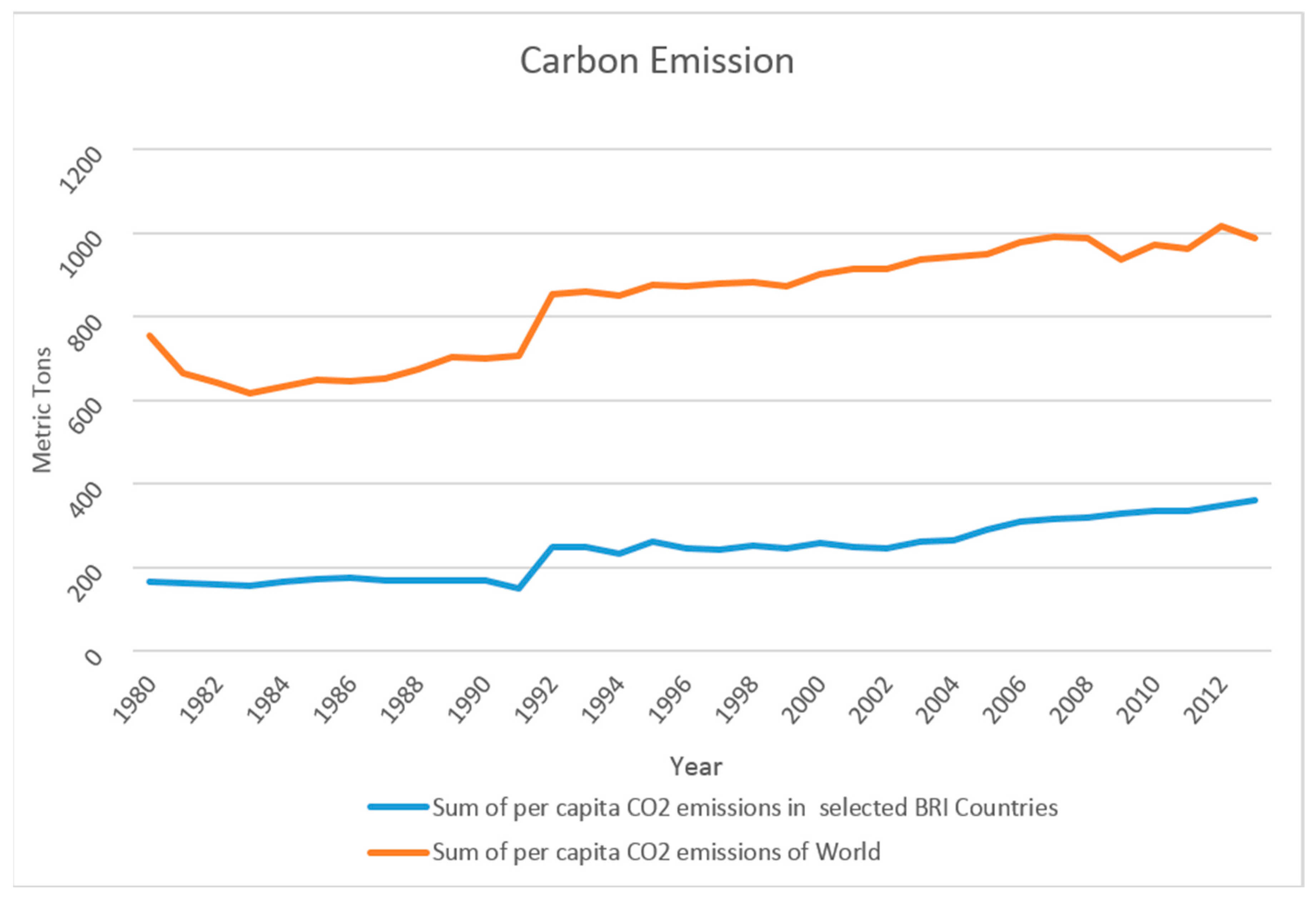Figure 1 presents the comparison of carbon emissions for selected BRI countries and the world, indicating that the sum of carbon emissions has increased over the last few years. The upward trend for carbon emissions in BRI economies, as well as in the world, may massively threaten future ecological quality. In 1980, the scale of CO₂ emissions on the world level experienced a small decline, but then surged until 2012. BRI economies have the same intensity trend in CO₂ emissions. If only counting China, the respective level of global CO₂ emissions in BRI nations has reached approximately 61.4% [17]. Furthermore, the proportion of energy-intensive CO₂ emissions in BRI economies is about 80%, indicating the crucial contributions of the energy sector to environmental degradation. On this basis, it is hard to escape the conclusion that BRI projects are going to harm the environment, as well as being beneficial for economic growth. In addition, a few researchers have also asserted that the “global shifting wave” of BRI projects would produce severe undesirable influences on indigenous resources and ecosystems [18]. As such, it has become one of the major issues affecting the success of BRI projects in bounded economies.

Previous studies have reported a significant relationship between economic growth, financial development, and carbon emissions. Grossman and Krueger [20] presented the well-known environmental Kuznets curve (EKC), which is an inverted U shape. It states that during the initial stage of economic growth, policymakers mostly focus on growth rather than environmental degradation. The second stage of economic growth reduces the pace of pollutant emissions. In the third stage, policymakers introduce environmentally friendly policies such as industrial treatment plants, renewable energy consumption, energy-efficient technologies, etc., which lower GHG emissions. Previous studies can be divided into two categories. Some support the EKC hypothesis [9,21,22,23,24]. The authors in [24] analyzed panel data from 40 Asian countries, and their estimations confirmed the inverted U-shaped curve. Likewise, [21] confirmed evidence of the EKC hypothesis in the case of 36 high-income countries. By contrast, some researchers report the nonexistence of the EKC hypothesis. The authors in [25,26,27,28] attempted to examine the EKC hypothesis and reported conflicting results. In the same vein, [25] used the panel data approach and confirmed weak evidence of the EKC hypothesis. Later, the findings in [27] also negated the EKC hypothesis. There are several key reasons for these conflicting pieces of evidence, such as there being no fundamental environmental theory, but most of the research is based on Kuznets’ seminal work examining the inverted U-shaped curve [29]. Other significant reasons for a variation in the EKC results are the use of different datasets, and the utilization of various econometric techniques and conditions. However, [10,11] suggested that the ideal way to examine the existence of the EKC hypothesis across the world is to remove cross-sectional independence, normalize the responses for each country and the use the same econometric techniques to analyze the short-run and long-run relationships.

Recent literature has extended the EKC model by incorporating different factors such as technological innovation, financial development, industrialization, urbanization, etc. The authors in [15,30] found a significant and positive relationship between urbanization and energy consumption, which further leads to higher carbon emissions. The findings show that more than 50 percent of the population of the world is living in urban areas that are responsible for around 70 percent of GHGs. Some researchers have reported similar results [31,32,33,34,35,36,37,38,39,40,41,42]. Reference [34] reported that an increase in family income and family size has led to an increase in carbon emissions in selected regions of China. The authors in [43] documented that higher urbanization is one of the main causes of carbon emissions. The authors in [34] investigated urban- and rural-based household carbon emissions and confirmed that urban-based carbon emissions are higher than rural-based carbon emissions, with 0.50 tCO₂ and 0.22 tCO₂, for urban- and rural-based emissions, respectively. References [44,45] suggested that the government should increase forest investment, implement sound policies and adequately audit resources to control the environmental degradation process. Reference [5] used three-data envelopment analysis to examine the total factor energy efficiency of 35 BRI countries. The findings showed that countries with low energy efficiency have higher emissions. The authors in [46] investigated the empirical relationship between energy consumption, income, carbon emissions, capital formation and labor. In the context of low carbon (CO₂) endorsement, it is necessary to place sufficient significance on efficient progress to attain harmonized and ecological sustainability in various segments, namely energy usage, trade, technological investment, urbanization, labor and capital speculation (financial development and gross fixed capital formation, etc.).

The previous literature misses the impact of BRI projects on economic growth, energy consumption patterns and their harmful effects on the environment. This is a gap in the existing literature, which implies that no novel research has been proposed to consider a panel investigation based on 47 BRI economies with a cross-country analysis. The noteworthy objective of the present fact-finding study is to validate the links between economic growth, energy consumption, urbanization, gross fixed capital formation, trade openness, financial development and carbon emissions (ecological degradation) across a panel of 47 BRI economies, using a time span from 1980 to 2016. Various panel unit root tests have been undertaken to identify the level of stationarity among the variables, and subsequently the stationary level of panel cointegration tests required to gauge the level of integration among them. Hence, the cointegration patterns of dynamic panel estimations (dynamic ordinary least square (DOLS) and fully modified ordinary least square (FMOLS)) were suggested to examine the long-run linkages among the subjected variables. Furthermore, pairwise panel Granger causative tests were employed to assess the pattern of the directional links from all regressors towards CO₂ emissions. In cross-country, long-run assessments, some mixed interactions have been determined from regressors towards CO₂. Based on retrieved estimations, there could be some policy implications for the full panel and individual countries, to address the energy, economy and ecological potentials and future encounters. Subsequently, the estimations have led to solid strategic recommendations and inferences for governments and policy-makers in terms of sound governance, waste management plans, renewable energy dependency and the undertaking of necessary decisions to sanitize the environment.

Section 2 comprises research methodologies, data collection, and details; Section 3 contains the results and discussion. Section 4 deals with conclusions, policy implications and recommendations.

2. Research Methods and Data Explanation

2.1. Variables and Data Informers

The current investigation involved those 47 BRI countries depicted in Appendix B,

Table A2. List of the 47 Belt and Road Initiative countries.

Sr. No	Country	Sr. No	Country	Sr. No	Country
1	Albania	17	India	33	Pakistan
2	Armenia	18	Indonesia	34	Philippines
3	Azerbaijan	19	Iran	35	Romania
4	Bahrain	20	Israel	36	Poland
5	Bangladesh	21	Jordan	37	Russian
6	Belarus	22	Kazakhstan	38	Saudi Arabia
7	Bosnia	23	Kyrgyz Rep.	39	Slovak Rep
8	Bulgaria	24	Kuwait	40	Sri Lanka
9	Cambodia	25	Lebanon	41	Tajikistan
10	Colombia	26	Macedonia	42	Thailand
11	China	27	Malaysia	43	Turkey
12	Croatia	28	Moldova	44	Ukraine
13	Czech Rep	29	Mongolia	45	UAE
14	Egypt	30	Myanmar	46	Vietnam
15	Georgia	31	Nepal	47	Yemen, Rep.
16	Hungary	32	Oman	48

Source: World Bank Classification (http://data.worldbank.org/about/country-classifications/country-and-lending-groups).

. The panel selection of the 47 economies was determined based on the availability of a dataset from the World Development Indicators [19]. The BRI was initiated by the Chinese government, to articulate the slogan “Going global through bilateral relationships” [47,48]. The fruition and sustainability of an economy depends on all sectors participating in economic activities. Such contributions could comprise capital investment, urbanization, trade openness, labor operations, gross domestic product (GDP), ecological sustainability and energy utilization. Furthermore, these are all mandatory in order to accelerate economic progress and achieve sustainability. The BRI encompasses more than 68 countries, allowing an understanding of the demand and supply of energy in project operations, sustainable development, ecological sustainability, business and trade collaboration, infrastructure development and much more. Therefore, based on the discussions mentioned earlier, it is essential to assess future challenges and outlooks for the BRI to succeed in all areas. Thus, the present study uses carbon emissions (CO₂) as a predicted variable to determine ecological sustainability. The independent variables are specified as energy consumption, economic growth (GDP), urbanization, financial development, gross fixed capital formation and trade openness, as shown in

Table 1. Variable descriptions and data sources.

Variables	Elaboration	Data Source
Carbon emission (CO2)	Metric tons of CO2 equivalent per capita	WDI
Energy consumption (ECON)	Energy usage (kg of oil equivalent per capita)	WDI
Gross domestic product (GDPPC)	GDP per capita (constant at 2010 US $)	WDI
Financial development (FD)	Domestic credit to private sector as a% of GDP	WDI
Gross Fixed Capital Formation(GFCF)	Gross Fixed Capital Formation% of GDP	WDI
Urbanization (URB)	Urban population% of the total population	WDI
Trade Openness (TRADE)	Total Exports plus imports% of GDP	WDI

Note: Author’s tabulation.

with a relevant explanation. The study employed the logarithmic format of variables to obtain small coefficients and interpret estimates smoothly with relevance to CO₂ emissions, as determined by [9,49,50,51,52,53,54,55,56].

2.2. Econometric Methodology

The links between CO₂ emissions, ECON, FD, GDPPC, FD, URB, GFCF, and TRADE are shown by a simple equation taking “i” as the explicit BRI full panel candidate country and “t” as time for 47 BRI economies. In the illustration, it is essential to detect the unit root for subjected variables when they are either stationary, in the first difference or in the second difference. Usually, there are many unit root tests for the individual time series dataset (ADF, PP, KPSS, and GLS, among others). The tests in [57,58,59] are recognized to have low efficacy compared to the alternative state of stationary series, used predominantly for small illustrations. The panel data provides a greater number of points in the dataset, increasing the degrees of freedom (dof) and decreasing the multicollinearity among the predictor regressors. As such, it tolerates further authoritative statistical tests and the values under test statistics asymptotically track a normal dispersion, as a replacement for nonconventional dispersion. There are various tests available for the panel unit root, such as in references [60,61,62,63]. In this study, four different unit root tests were used, including Levin, Lin and Chu (LLC) [62], I’m, Pearson and Shin (IPS) [63], Augmented Dickey Fuller (ADF) Fisher Chi-square, and panel Phillips and Perron (PP) unit root tests. Furthermore, if the panel datasets assert the same level of integration under the unit root estimators with significance spot, then panel cointegration would be pulsed via various cointegration tests in BRI grouped economies. Moreover, this further allows for cointegration inspection among the predicted variables and regressors under the Pedroni cointegration test [64,65,66]. The cross-checking was done with a Johansen Fisher panel cointegration test pioneered by the authors in [67], later upgraded in reference [60], here applied to evaluate the long-run cointegration among the subjected variables. The Kao-based residual cointegration test was also employed to authenticate the estimations, which were derived from the Pedroni and Johansen Fisher panel cointegration analyses correspondingly. Subsequently, dynamic panel modeling, including fully modified ordinary least square (FMOLS) and dynamic OLS (DOLS) models operate explicitly to identify the links from the regressors to the dependent variable. However, the robustness of the FMOLS and DOLS models were metered by exerting panel pooled regression, fixed effect, and random effect models harmoniously. To sum up, various problem-solving tests such as the Jarque–Bera test and normality tests declared the estimations’ robustness.

2.2.1. Model Identification

The predicted variables and regressors in the investigation are rendered in Equation (1), which has been tracked by different investigators, see [9,40,49,50,51,52,54,55,56]. The equation is expressed as below:

$$C{O}_2=f\left(EC,GDP,FD,GFCF,TRADE, URB\right)$$

(1)

The reformation of Equation (1) has been carried out to grasp all subjected variables and transform them into natural logarithms. Hence, the problem of heteroscedasticity and high coefficient estimators could be resolved. Equation (2) is specified as below:

$${C{O}_2}_{i,t}=\alpha +{\beta }_{1}lnECO{N}_{i,t}+{\beta }_{3}lnGD{P}_{i,t}+{\beta }_{2}lnF{D}_{i,t}+{\beta }_{4}lnGFC{F}_{i,t}+{\beta }_{5}lnTRAD{E}_{i,t}+{\beta }_{5}lnUR{B}_{i,t}+{\epsilon }_{i,t}$$

(2)

The representation in Equation (2) magnified the predicted variables and regressors; “$ln$” suggests a natural logarithm; and “i” and “t” pronounced the country-explicit statistics and time in the dataset correspondingly. Moreover, “$\alpha$” is an intercept; entire $\beta$ illustrates the relevant country-explicit parameters in the subjected regressors; and “${\mathsf{\epsilon }}_{\mathrm{i},\mathrm{t}}$” is the innovativeness or error term in this investigation.

2.2.2. Panel Unit Root Tests

An early inspection of the dataset outlined by four-panel unit root tests (LLC, IPS, ADF, and PP) identifies the stationary level of the presented variables. The engrossed longitudinal dataset suggests that a larger number of time occurrences may foster a degree of freedom and cause the delinquents of the multicollinearity in the least square equation to trickle. The unit root tests of IPS and LLC are grounded on following model equation:

$$\Delta y_{i,t}={\alpha }_i+{\beta }_i{y}_{i,t-1}{\displaystyle \sum }_{j=1}^{pi}{\rho }_{ij}\Delta y_{i,t-j}+{\epsilon }_{i,t} i=1,\dots t=1,\dots T$$

(3)

Equation (3) incorporates $y_{i,t}$ the longitudinal dataset for $“i”$ economy and $“t”$ time period, $“pi”$ stipulates the lag operator in the regression equation. $“{\epsilon }_{i,t}”$ particularizes the innovativeness or error terms for every individual BRI economy and time span, for the normal random distribution of the predicted variables and regressors. Null and alternative hypothesis were established to trail the stationarity properties of variables under the four different panel unit root tests (LLC, IPS, ADF and PP); likewise, $H_0$ = Null hypothesis $p$ = 0 for the full panel comprises economies “i” (contains series with a unit root); on the contrary $H_1$ = Alternative hypothesis $p$ < 0 with a minimum of one or a few “i” (does not contain dataset series with a unit root). Similarly, the hypothesis will be accepted or rejected by relating with asymptotically predetermined table values. Moreover, the LLC test for the unit root is grounded in Equation (3), nonetheless it considers autoregressive and moving average (ARMA) terms and their coefficients coherently in diagonal to the subjected variables.

2.2.3. Panel Cointegration Tests

According to the inference, under the panel unit root examination the dataset series could either be steady at level I (0) or at first difference I (1). Likewise, if the dataset series are stationary at that level, that would prompt the application of conventional OLS panel procedures, but if the series are stationary at first difference, we should explore the cointegrating association between the predicted variables and regressors. The order of cointegration (1, 1) acquired as two variables, may be incoherently non-stable, but its unveiled, linear-patterned stationarity is positioned between them, indicating that panel cointegration exists among the variables. The panel cointegration tests devised by [64,65] have been utilized to gauge the stationarity position between the variables as employed by [56,68,69,70]. Hence, the variables consistently integrated at the first-order I (1) will sequentially determine whether the data series has cointegration. The test for panel cointegration contains seven residual-based statistical tests to elect the presence of long-run links among the data series. These residual-based regression statistics comprise panel rho-statistic, panel v-statistic, panel ADF-statistic, panel PP-statistic, group rho-statistic, group PP-statistic, and group ADF-statistics. The hypothesis of the Pedroni cointegration test and null hypothesis is constructed as H0: there is no cointegration association for all “i”; in contrast, the alternative hypothesis is determined as H1: there is a cointegration relationship for all “i”. In the event that the panel statistics have a larger positive value as their weight, while in contrast the statistics have a larger negative value as their weight, the “H0” hypothesis denotes that there is no cointegration among the two dataset series, and it is discarded, it is inferred in conclusion that there is a long-run connection between the subjected predicted variables and regressors.

The Pedroni cointegration test equation is as follows:

$$\begin{array}{c}{C{O}_2}_{i,t}=\alpha +{\delta }_{i}t+{\beta }_{1}lnECO{N}_{i,t}+{\beta }_{3}lnGD{P}_{i,t}+{\beta }_{2}lnF{D}_{i,t}+{\beta }_{4}lnGFC{F}_{i,t}+{\beta }_{5}lnTRAD{E}_{i,t}\\ +{\beta }_{5}lnTRAD{E}_{i,t}+{\epsilon }_{i,t} i=1,\dots t=1,\dots T\end{array}$$

(4)

In Equation (4), the footing description of the cointegration test has been exhibited, where $“{\alpha }_i”$ is the country-specific constant, and the deterministic tendency is ${\delta }_{i}t$ for corresponding single countries in the full panel of 47 BRI economies. The standardized evidence is distributed asymptotically as values extracted in the Pedroni cointegration test. As a result, the Pedroni equation format could be as follows:

$$\sqrt{\frac{N_{N,T}^{\prime }-\mu \sqrt{N}}{\sqrt{V}}}\to N\left(0,1\right)$$

(5)

Equation (5) discloses $\mu$, and V uncovered Monte Carlo (MC)-shaped and variation terms, respectively. The opening four statistics embody panel statistics or within-dimension valuation, while the far ahead three symbolizes (cluster) statistics tests or between dimensions.

We also operate the Johansen Fisher panel cointegration test to authorize outcomes from the Pedroni cointegration test founded on the individual intensive Johansen cointegration test devised by [67]. The test estimations found that there exists long-run cointegration among the data variables. Furthermore, the Pedroni and Johansen Fisher cointegration tests were counterchecked by employing the Kao residual-based cointegration test.

2.3.4. Dynamic Panel Modeling

The study engaged the [65,66,71] panel fully modified OLS (FMOLS) and dynamic OLS (DOLS) to measure the long-run cointegrating relationship between regressors and the predicted variable (CO₂). The principal motivation for exploiting the dynamic economic models FMOLS and DOLS takes into consideration the correlational setbacks among the panel intensive-error terms.

Indeed, all studied variables are transformed into logarithms, to standardize the results. The following equations will determine and measure the FMOLS and DOLS estimations over the study hypothesis:

$${\widehat{\beta }}_{NT}=\left[\frac{{{\displaystyle \sum }}_{i=1}^N{{\displaystyle \sum }}_{t=1}^T\left(x_{it}-{\overline{x}}_i\right)\left(y_{it}-{\overline{y}}_i\right)-T{\widehat{\gamma }}_i}{{{\displaystyle \sum }}_{t=1}^T{\left(x_{it}-{\widehat{x}}_i\right)}^2}\right]$$

(6)

where

$${\widehat{\gamma }}_i={\widehat{\Gamma }}_{21i}+{\widehat{\Omega }}_{21i}^0-\frac{{\widehat{\Omega }}_{21i}}{{\widehat{\Omega }}_{21i}}\left({\widehat{\Gamma }}_{22i}+{\widehat{\Omega }}_{22i}^2\right)$$

(7)

and

$${\widehat{\Omega }}_i={\widehat{\Omega }}_i^0+{\widehat{\Gamma }}_i+\widehat{\Gamma }{\prime }_i$$

(8)

The ${\widehat{\Omega }}_i$ term displays the matrix of long-run stationarities following by ${\widehat{\Omega }}_{21i}^0$, which deal with the covariance amid stationary error terms. Moreover, the ${\widehat{\Gamma }}_i$ illustrates the corrected covariance term among the regressor variables.

2.3.5. Heterogeneous Panel Causality Test

The subsequent phase in determining the links between the variables outline the track of causative association by Granger causality examination. Here, the heterogeneous Granger causality test described by [72] and centered on Wald asymptotical values will be exploited to extract the estimators. The benefit of this assessment is that it considers the reliance on individual economies and heterogeneity. Furthermore, it can function when the time length (T) is greater or lesser than the cross-country length (N). In this technique, the examination functions with two regular dataset series, and if the dataset series handled in the examination are not steady, they should be steadied by taking their divergence (first difference). During the pairwise heterogeneous Granger causality inspection, “H0” is the null hypothesis and “H1” is an alternative hypothesis.

H0: 

βi = 0 ^i = 1, …, N (there is no causative connection from x to y).

H1: 

βi = 0 ^i = 1, …, N1; βi ≠ 0 ^i = N1 + 1, N1 + 2, …, N (there is a causative connection from x to y).

3. Empirical Results and Discussion

The empirical valuations were obtained by using the FMOLS and DOLS modeling. A total of 47 BRI economies were considered, concerning the total energy, economy and ecological sustainability challenges and prospects across the full panel and in the cross-country examinations, illuminating the long-run estimators for country-specific policy decisions and implications.

3.1. Descriptive Statistics

Table 2. Descriptive statistics.

	CO2	ECON	GDPPC	GFCF	FD	TRADE	URB
Mean	0.766	6.115	7.107	19.745	30.525	68.450	53.130
Median	0.681	6.810	7.884	21.264	24.218	67.499	54.355
Maximum	3.580	9.426	11.641	65.560	166.504	251.139	98.358
Minimum	−3.560	0.000	0.000	0.000	0.000	0.000	6.091
Std. Dev.	1.376	2.662	2.950	11.082	30.612	47.637	21.559
Skewness	−0.280	−1.494	−1.542	−0.269	1.341	0.453	−0.033
Kurtosis	2.839	4.106	4.455	3.386	4.993	2.948	2.164
JB Test	24.305	727.237	832.790	31.380	799.506	59.061	50.410
Prob.	0.000	0.000	0.000	0.000	0.000	0.000	0.000
Obs.	1719	1719	1719	1719	1719	1719	1719

Note: Author’s tabulation where; CO₂ denotes carbon emissions; ECON depicts the Energy consumption; GDPPC shows Gross domestic product per capita; FD represents Financial development; GFCF indicates Gross Fixed Capital Formation; URB identifies Urban population; and TRADE signifies Trade Openness. Furthermore, JB Test reveals the Jarque-Bera test for normality; Std. Dev. denotes standard deviation; Prob. defines the probability of JB. test and Obs. illustrates the number of observations in the dataset.

displays the summary information for all the studied variables dynamically. It covers 47 cross-sections and 37-time spans that encompass, in total, 1719 observations. The variables were principally transformed into natural logarithms to sidestep undesirable shocks; similarly, these estimations might also have unveiled setbacks to the reliability of the current study. The mean, median, maximum and minimum values are displayed in Table 2. These signify the ranges and dispersion of the dataset. The standard deviation elaborates that how much a specific time series data point diverges from its mean value. The skewness and kurtosis of the dataset were observed, where the skewness reveals the degree of asymmetry in the dataset information and kurtosis whether the dataset series distribution has peaks or is flat. There are three points of skewness; normal = 0, positive = long right tail (higher statistics values), and negative = long left tails (lower statistics values). In the same way, kurtosis also has three positions, namely, Mesokurtic = normal distribution (value of kurtosis is 3), Leptokurtic = peaked curve (positive kurtosis leads that are higher than 3) and Platykurtic = flatted curve (negative kurtosis leads that are lower than 3). The Jarque-Bera test (JB test) assesses the normality of the data series in the subjected study analysis.

3.2. Correlational Statistics

Table 3. Correlational statistics.

Correlation
Probability	CO2	ECO	GDPPC	GFCF	FD	TRADE	URB
CO2	1
	-----
ECON	0.5653 ***	1
	0.0000	-----
GDPPC	0.4232 ***	0.5044 ***	1
	0.0000	0.0000	-----
GFCF	0.2096 ***	0.3251 ***	0.5754 ***	1
	0.0000	0.0000	0.0000	-----
FD	0.2592 ***	0.1801 ***	0.4089 ***	0.4233 ***	1
	0.0000	0.0000	0.0000	0.0000	-----
TRADE	0.3652 ***	0.3602 ***	0.5422 ***	0.5088 ***	0.4523 ***	1
	0.0000	0.0000	0.0000	0.0000	0.0000	-----
URB	0.7690 ***	0.3061 ***	0.3052 ***	0.0430 *	0.2125 ***	0.2866 ***	1
	0.0000	0.0000	0.0000	0.0746	0.0000	0.0000	-----

Note: Author’s tabulation where; CO₂ denotes carbon emissions; ECON depicts the Energy consumption; GDPPC shows Gross domestic product per capita; FD represents Financial development; GFCF indicates Gross Fixed Capital Formation; URB identifies Urban population; and TRADE signifies Trade Openness. *, **, *** indicates that statistics are significant at the 10%, 5% and 1% level of significance, respectively.

shows the correlational statistical values of the subjected variables and their respective probability. It seems that all variables are significantly correlated with CO₂ emissions in 47 BRI economies. Indeed, urbanization and energy consumption have more than 50% influence on environmental quality, whereas the GDPPC, trade openness, financial development and gross fixed capital formation were 42.32%, 36.52%, 25.92 and 20.96%, respectively. This implies that energy consumption and urbanization damage the environment much more adversely than other regressors.

3.3. Data Diagnostics

Panel Unit Root Tests

The panel unit root tests (LLC, IPS, ADF, and PP) were used to analyze the stationarity position of the studies dataset. The retrieved estimations are reported in

Table 4. Panel unit root test.

At Level
Regions	Methods	CO2	ECON	GDPPC	GFCF	FD	TRADE	URB
Full panel 47 countries	LLC	2.563	12.148	11.925	−4.340	7.842	−2.184 **	12.961
	IPS	2.801	4.242	6.416	−4.162	9.218	−0.966	−0.150
	ADF	80.662	60.327	60.133	146.992	38.392	104.548	122.581 **
	PP	73.656	34.617	117.395 *	128.598	38.693	115.163 *	380.958 ***
1st Difference
Full panel 47 countries	LLC	−36.90 ***	−31.11 ***	−149.7 ***	−38.36 ***	−25.1 ***	−33.410 ***	−6.354 ***
	IPS	−31.31 ***	−22.44 ***	−52.55 ***	−32.15 ***	−25.4 ***	−33.010 ***	−4.671 ***
	ADF	957.30 ***	776.28 ***	706.47 ***	838.42 ***	761.33 ***	970.871 ***	310.124 ***
	PP	1031.750	884.77 ***	768.11 ***	979.89 ***	827.96 ***	1045.85 ***	546.27 ***

Note: Author’s estimations where; CO₂ denotes carbon emissions; ECON depicts the Energy consumption; GDPPC shows Gross domestic product per capita; FD represents Financial development; GFCF indicates Gross Fixed Capital Formation; URB identifies Urban population; and TRADE signifies Trade Openness. Furthermore, LLC indicates Levin, Lin and Chu unit root test; IPS depicts I’m, Pearson and Shin; ADF illustrates ADF Fisher Chi-square and PP displays the Phillips and Perron unit root test. *, **, *** indicates that statistics are significant at the 10%, 5% and 1% level of significance, respectively.

. All variables under the LLC, IPS, PP and ADF tests were stable and stationary at first difference. This indicates that all variables are stationary at first difference, which prompts exploration of the cointegration state among predicted variables and regressors. However, under the ADF and PP unit root tests, urbanization had significant probability and trade also had significant probability at 10%. On the other hand, as the variables were converted into the first difference, these all become stable. Under all unit root tests, the null hypothesis was discarded (H0 = there is a unit root) and the alternative hypothesis accepted (H1 = there is no unit root) to support the first-order stationarity inferences. At first the descriptive statistics and panel unit root estimations were probed to assess the probable cointegration position. Then, there was a move for the engagement of different cointegration tests, such as Pedroni panel cointegration tests, the Fisher and Johansen and Fisher cointegration test and the Kao-based residuals test, as reported in [56,70,73].

Pedroni cointegration permits greater T and N to scrutinize the cointegrated links among the disclosed variables. The model computed seven tests based on individual and cluster groups, where the probability significance determined the level of cointegration among the variables. In

Table 5. Pedroni panel cointegration test.

Alternative Hypothesis: Common Auto-Regressive (AR) Coefficients
Within-dimension
	Statistic	Prob.	Statistic	Prob.
Panel v-Statistic	1.96206	0.025 **	−3.8078	1.000
Panel rho-Statistic	3.7788	1.000	3.766	1.000
Panel PP-Statistic	−6.5950	0.000 ***	−6.4180	0.000 ***
Panel ADF-Statistic	−5.7340	0.000 ***	−6.4840	0.000 ***
Alternative hypothesis: individual AR coefficients
(between-dimension)
	Statistic	Prob.
Group rho-Statistic	5.3726	1.000
Group PP-Statistic	−9.1704	0.000 ***
Group ADF-Statistic	−4.3975	0.000 ***

Note: *, **, *** indicates that statistics are significant at the 10%, 5% and 1% level of significance, respectively.

, seven tests overruled the null hypothesis (H0), and ensured that at I (1, 1) the variables have long-run cointegration. In addition, the Johansen and Fisher (JF) panel cointegration test was employed and reported in

Table 6. Johansen fisher panel cointegration test cointegration rank test (trace and maximum eigenvalue).

Hypothesized	Fisher Statistics		Fisher Statistics
No. of CE (s)	(from Trace Test)	Prob.	(Max-Eigen Test)	Prob.
None	1883.000	0.000 ***	1897.000	0.000 ***
At most 1	1146.000	0.000 ***	607.000	0.000 ***
At most 2	629.8	0.000 ***	336.2	0.000 ***
At most 3	360.5	0.000 ***	188.1	0.000 ***
At most 4	233.4	0.000 ***	144.3	0.001 ***
At most 5	166.7	0.000 ***	130.7	0.007 ***
At most 6	171.6	0.000 ***	171.6	0.000 ***

Note: “CE” denoted, Cointegration Equations. ***, indicates that statistics are significant at 1% level.

, to authenticate and align the Pedroni-based panel cointegration outcomes. The results of the JF cointegration test are shown in Table 6, suggesting the discarding of the null hypothesis (H0) under that particular test, meaning that there is no cointegration among the variables. Equally, these two tests affirm and ensure that there is long-run linear combination between the variables, as a clue for long-term panel cointegration. Finally, the Kao-based residual cointegration test was used as an additional certification to obtain strong and solid results for long-run cointegration, which are presented in

Table 7. Kao test for residual cointegration.

Null Hypothesis	No Cointegration
Kao t-Statistic	Probability
−5.952	0.000

. We found a result of −5.952 *** when using Kao-based statistics (−5.952 ***), which suggests that the previous two cointegration tests were efficient and warrant additional authentication.

3.4. Dynamic Panel Modeling

The panel estimations of the cointegration tests validated the long-run cointegration among the variables. It likewise suggests the application of fully modified OLS (FMOLS) and dynamic OLS (DOLS) for stable results [65,66,71]. DOLS and FMOLS were operated to test the study hypothesis and acknowledge the desired links. The empirical estimation in

Table 8. Panel long-run estimation under fully modified and dynamic OLS (DOLS and FMOLS).

Predicted Variable	CO2 Emissions/Environmental Degradation
	Panel (FMOLS)		Panel (DOLS)
Regressors	Coefficient	t-Statistic	Coefficient	t-Statistic
ECON	0.16259 ***	18.0931	0.112086 ***	6.7634
GDPPC	0.040417 ***	3.643503	0.038047 ***	2.67892
GFCF	0.012342 ***	4.302308	0.015532 ***	4.59378
FD	0.005335 ***	4.18017	0.00362 ***	2.78995
TRADE	−0.00537 ***	−6.544434	−0.00553 ***	−5.47391
URB	0.030532 ***	6.620429	0.039617 ***	7.17279
Observations	1669		1569
R2	0.882718		0.987315
Adjusted-R2	0.878944		0.970313

Note: Author’s estimations where; CO₂ denotes carbon emissions; ECON depicts the Energy consumption; GDPPC shows Gross domestic product per capita; FD represents Financial development; GFCF indicates Gross Fixed Capital Formation; URB identifies Urban population; and TRADE signifies Trade Openness. *, **, *** indicates that statistics are significant at the 10%, 5% and 1% level of significance, respectively.

reveals that the energy consumption, financial development, gross fixed capital formation, urbanization, and gross domestic product positively and significantly affect the ecological situation (increase in CO₂ emissions). On the other hand, trade openness has no adverse effect on ecological status in the 47 BRI economies. Using FMOLS, we found that a 1% rise in energy utilization, economic growth, financial development, gross fixed capital formation and urbanization leads to changes in ecological degrading (CO₂ emissions), with (0.16259 ***), (0.040417 ***), (0.012342 ***), (0.005335 ***) and (0.030532 ***), respectively. Likewise, trade openness has a negative impact on ecological status. The FMOLS estimations suggest that 47 BRI economies may have set up some policies that are controlling mutual trade openness and its adverse effect on ecological sustainability, but in contrast, others indicate alarmingly mounting pressures on ecological degradation for the 47 BRI economies. For the success of the BRI, censured actions must be taken, and governments need to adopt robust policies to reduce ecological degradation. Furthermore, the DOLS model produced the same estimates as reported for FMOLS, where energy utilization, economic growth, gross fixed capital formation, financial development, and urbanization patterns vary in terms of their effect on ecological degradation (CO₂ emissions). Similarly, trade openness has a negative influence on ecological status. Overall, the summary of the results of DOLS, and FMOLS suggests that in the 47 BRI countries, energy consumption highly based on oil, coal, and gas (non-renewable energy sources) is a threat to the ecological sustainability of BRI projects in the future. Does every nation need a high economic growth rate, no matter how it is achieved? The attainment of a high GDP in developing, emerging and low-developing economies has recently unfavorably affected environmental sustainability. Most economies under BRI are dependent on investment but not on green-intensive investment. Popular awareness of green investment may urge the scale of economic growth without deteriorating the environment. In the meantime, urbanization should be controlled in a way that will not influence ecological sustainability or its position. This study draws similar inferences to [8,9,25,40,49,50,51,52,55,56,70,74].

3.5. Dumitrescu Hurlin Panel Heterogeneous Causality Test

A panel Granger causality test based on heterogeneity, pioneered by [72], identified the causative links among the variables in the panel of 47 BRI economies. The results of the panel Granger causality test are shown in

Table 9. Pairwise Dumitrescu–Hurlin panel causality tests.

Null Hypothesis	W-Stat.	Zbar-Stat.	Prob.
ECON does not homogeneously cause CO2	2.5845	6.5894 ***	0.0000
CO2 does not homogeneously cause ECON	132.626	570.342 ***	0.0000
GDPPC does not homogeneously cause CO2	1.78912	3.14126 ***	0.0017
CO2 does not homogeneously cause GDPPC	17.4198	70.9029 ***	0.0000
GFCF does not homogeneously cause CO2	2.16896	4.77437 ***	0.0000
CO2 does not homogeneously cause GFCF	2.24507	5.10369 ***	0.0000
FD does not homogeneously cause CO2	1.79336	3.15877 ***	0.0016
CO2 does not homogeneously cause FD	4.65403	15.5583 ***	0.00000
TRADE does not homogeneously cause CO2	2.05119	4.27686 ***	0.0000
CO2 does not homogeneously cause TRADE	1.33402	1.16806	0.2428
URB does not homogeneously cause CO2	2.0885	4.43914 ***	0.0000
CO2 does not homogeneously cause URB	7.92282	29.7319 ***	0.0000
GDPPC does not homogeneously cause ECON	2.01748	4.13126 ***	0.0000
ECON does not homogeneously cause GDPPC	302.794	1308.05 ***	0.0000
GFCF does not homogeneously cause ECON	2.0842	4.40761 ***	0.0000
ECON does not homogeneously cause GFCF	5.09723	17.445 ***	0.0000
FD does not homogeneously cause ECON	2.3183	5.43411 ***	0.0000
ECON does not homogeneously cause FD	5.87297	20.8417 ***	0.0000
TRADE does not homogeneously cause ECON	2.01295	4.1111 ***	0.0000
ECON does not homogeneously cause TRADE	1.78924	3.14134 ***	0.0017
URB does not homogeneously cause ECON	2.20207	4.93148 ***	0.0000
ECON does not homogeneously cause URB	13.1911	52.5709 ***	0.0000
GFCF does not homogeneously cause GDPPC	1.21968	0.66684	0.5049
GDPPC does not homogeneously cause GFCF	4.4179	14.5056 ***	0.0000
FD does not homogeneously cause GDPPC	4.71034	15.8024 ***	0.0000
GDPPC does not homogeneously cause FD	2.31776	5.43178 ***	0.0000
TRADE does not homogeneously cause GDPPC	1.45646	1.69881 ***	0.0894
GDPPC does not homogeneously cause TRADE	3.0435	8.57836 ***	0.0000
URB does not homogeneously cause GDPPC	8.48795	32.1818 ***	0.0000
GDPPC does not homogeneously cause URB	26.2417	109.147 ***	0.0000
FD does not homogeneously cause GFCF	1.77286	3.05957 ***	0.0022
GFCF does not homogeneously cause FD	4.0814	13.0471 ***	0.0000
TRADE does not homogeneously cause GFCF	3.14244	8.98575 ***	0.0000
GFCF does not homogeneously cause TRADE	2.80657	7.53253 ***	0.0000
URB does not homogeneously cause GFCF	2.02434	4.14861 ***	0.0000
GFCF does not homogeneously cause URB	11.4119	44.7685 ***	0.0000
TRADE does not homogeneously cause FD	4.31992	14.1088 ***	0.0000
FD does not homogeneously cause TRADE	1.24132	0.76571	0.4438
URB does not homogeneously cause FD	2.9404	8.1306 ***	0.0000
FD does not homogeneously cause URB	14.1335	56.6468 ***	0.0000
URB does not homogeneously cause TRADE	2.54725	6.42721 ***	0.0000
TRADE does not homogeneously cause URB	27.2547	113.53 ***	0.0000

Note: Author’s estimations where; CO₂ denotes carbon emissions; ECON depicts the Energy consumption; GDPPC shows Gross domestic product per capita; FD represents Financial development; GFCF indicates Gross Fixed Capital Formation; URB identifies Urban population; and TRADE signifies Trade Openness. W-stat denotes Wald statistics, Zbar statistics and their probability. *, **, *** indicates that statistics are significant at the 10%, 5% and 1% level of significance, respectively.

. The heterogenous causality test estimations for the 47 economies offer divergent results. The causative estimates suggest bi-directional links from energy consumption, economic growth, financial development, urbanization and gross fixed capital formation towards CO₂ emissions (environmental quality), except for trade openness, which has unidirectional ties with environmental quality. Moreover, the heterogeneous panel test determined that an increase in regressors significantly causes a worsening of the environment quality. The nature of such estimations reveals that most of the economies in the BRI are emerging and less-developed countries are currently trying to increase their economic growth, mutual trade cooperation, infrastructural development and much more, but have not yet approached how encourage growth without having a negative effect on the environment. As such, BRI economies should introduce strong policies for solid governance as a whole, planning for mitigating the demand and supply of energy, BRI projects’ energy and ecological challenges and prospects, growing industrial production for mutual trade, policies for renewable energy dependency, forming industrial waste and water treatment plants and many others.

3.6. Country-Wise Long-Run Estimations

In the cross-country long-run estimations, dissimilar results were found, where the CO₂ emissions were intensely increased by economic growth in all countries and energy consumption in 30 countries, and other predictors testified some mixed interactions of economic indicators with CO₂ emissions at the country level. The long-run statistical evaluations of ecological degradation centered on an individual economy are presented in Table 7. The outcomes of all economies, from Albania to Yemen, in

Table 10. Cross-country analyses of the 47 BRI countries.

No	Variables	ECON		GDPPC		GFCF		FD		URB		TRADE		Constants (C)
	Country	Coff	Prob.	Coff	Prob.	Coff	Prob.	Coff	Prob.	Coff	Prob.	Coff	Prob	Coff.	Prob.
1	Albania	0.06835	0.0825	4.7912	0.0000	−0.0465	0.0008	−0.0172	0.2047	−0.1761	0.0000	0.0037	0.3501	−28.7720	0.0000
2	Armenia	0.07422	0.109	0.0155	0.0000	0.0004	0.9324	0.0071	0.0002	0.0532	0.1470	−0.0078	0.0040	−3.5692	0.1472
3	Azerbaijan	−0.08112	0.035	0.0478	0.0000	−0.0088	0.1032	0.0169	0.0352	−0.3453	0.0000	0.0116	0.0001	18.4960	0.0000
4	Bahrain	0.09499	0.031	0.2208	0.0000	−0.0347	0.0001	−0.0082	0.0614	−0.3249	0.0078	0.0006	0.7354	29.7019	0.0077
5	Bangladesh	−1.78442	0.0000	−0.0443	0.0000	0.0075	0.4128	0.0028	0.7355	0.1693	0.0000	0.0036	0.4522	5.9120	0.0216
6	Belarus	−0.19935	0.0000	0.0890	0.0000	0.0033	0.8548	−0.0047	0.5062	−0.0169	0.3644	0.0171	0.0000	1.0458	0.3640
7	Bosnia	−0.03283	0.7929	0.0550	0.0070	−0.0024	0.8947	0.0338	0.0024	−0.0951	0.4641	−0.0059	0.4778	3.6604	0.4595
8	Bulgaria	1.42527	0.0087	0.0862	0.0000	−0.0197	0.0388	−0.0051	0.1565	−0.2934	0.0000	0.0068	0.0077	8.8907	0.0035
9	Cambodia	0.08377	0.1305	−0.0044	0.0286	0.0035	0.9137	0.0145	0.0002	0.2035	0.0005	−0.0023	0.5245	−5.6522	0.0000
10	Colombia	0.17797	0.7197	0.0118	0.0000	0.0083	0.4514	0.0028	0.2748	−0.0338	0.1409	0.0132	0.1610	0.1982	0.9416
11	China	1.59254	0.0087	0.1674	0.0000	0.0148	0.4390	−0.0180	0.0036	−0.0626	0.1330	−0.0057	0.4205	−7.9947	0.0039
12	Croatia	−0.02417	0.7389	0.0438	0.0000	0.0367	0.0322	−0.0036	0.1651	−0.0607	0.1578	0.0008	0.9302	3.2041	0.1576
13	Czech Rep	−0.45642	0.0001	0.1336	0.0000	0.1846	0.0000	−0.0065	0.4240	0.2899	0.3120	0.0092	0.1612	−22.3540	0.3014
14	Egypt	1.12975	0.0000	0.0366	0.0000	0.0021	0.5024	0.0035	0.0006	0.2615	0.0000	0.0027	0.0025	−20.4076	0.0000
15	Georgia	0.19841	0.1767	0.0122	0.0138	−0.0140	0.0468	0.0045	0.3394	0.0113	0.9031	0.0033	0.1001	−2.3135	0.6248
16	Hungary	0.08042	0.007	0.0505	0.0000	−0.0406	0.0023	−0.0026	0.0215	−0.1321	0.0000	−0.0031	0.0002	10.1383	0.0000
17	India	−1.56199	0.0004	0.0551	0.0000	0.0338	0.0000	−0.0188	0.0000	0.4780	0.0000	−0.0085	0.0464	−3.6612	0.0019
18	Indonesia	0.78634	0.1172	0.0295	0.0000	−0.0233	0.0011	0.0027	0.1907	0.0182	0.2343	−0.0026	0.2298	−6.6737	0.0386
19	Iran	0.36146	0.1597	0.0875	0.0000	−0.0049	0.4018	−0.0011	0.7493	0.0368	0.0000	0.0032	0.1900	−5.7818	0.0044
20	Israel	−0.69081	0.1711	0.0899	0.0000	−0.0241	0.0136	0.0037	0.1051	0.1561	0.1903	0.0003	0.9286	−6.9458	0.2565
21	Jordan	0.04187	0.8087	0.0353	0.0000	0.0014	0.7318	−0.0024	0.5263	0.0354	0.0000	0.0022	0.0347	−3.0562	0.0435
22	Kazakhstan	−0.18647	0.0012	0.3277	0.0000	0.1135	0.0154	−0.0096	0.4111	−0.1119	0.3217	−0.0056	0.5456	6.2570	0.3212
23	Kyrgyz Re	−0.18647	0.0012	0.3277	0.0000	0.1135	0.0154	−0.0096	0.4111	−0.1119	0.3217	−0.0056	0.5456	6.2570	0.3212
24	Kuwait	0.28116	0.0000	0.2341	0.0000	−0.0048	0.7858	0.0168	0.0007	−0.4380	0.1086	−0.0568	0.0127	44.3577	0.1138
25	Lebanon	−0.04005	0.2453	0.0540	0.0000	0.0092	0.0943	0.0079	0.0560	0.0809	0.0088	−0.0052	0.0026	−7.0972	0.0047
26	Macedonia	0.03205	0.8365	0.0825	0.0001	−0.0334	0.4954	−0.0150	0.0523	0.0718	0.0523	0.0105	0.1470	−3.8303	0.5184
27	Malaysia	2.46630	0.0506	0.0795	0.0000	0.0085	0.4290	−0.0051	0.0016	−0.0284	0.5228	0.0032	0.0139	−20.7046	0.0111
28	Moldova	0.30634	0.0208	0.0490	0.0001	0.0446	0.0328	−0.0396	0.0005	0.0189	0.6790	−0.0223	0.0063	−0.6793	0.7393
29	Mongolia	−0.62794	0.611	0.0930	0.0000	0.0252	0.0061	0.0357	0.0307	−0.0681	0.4805	−0.0063	0.1472	8.5793	0.1145
30	Myanmar	1.79061	0.0000	−0.0083	0.0039	−0.0128	0.0000	0.0609	0.0000	−0.2685	0.0000	0.0038	0.2617	−5.0959	0.0000
31	Nepal	4.43851	0.0000	−0.0201	0.0000	0.0382	0.0070	0.0102	0.0046	−0.1808	0.0001	0.0121	0.0000	−28.0156	0.0000
32	Oman	0.13973	0.0809	0.0935	0.0047	0.0034	0.8096	0.0013	0.9244	0.0683	0.0028	−0.0062	0.6442	−5.0186	0.0049
33	Pakistan	1.94434	0.0000	0.0029	0.0562	−0.0021	0.8228	0.0053	0.0720	−0.0420	0.0629	−0.0067	0.0870	−11.9771	0.0000
34	Philippines	0.76211	0.0000	0.0051	0.0018	0.0087	0.0251	0.0067	0.0001	0.0205	0.0001	0.0012	0.1150	−7.5009	0.0000
35	Romania	−0.03298	0.3042	0.0663	0.0000	0.0105	0.0252	−0.0214	0.0000	0.0463	0.1534	−0.0152	0.0000	−0.4124	0.7974
36	Poland	0.08758	0.0000	0.1222	0.0000	−0.0324	0.0000	−0.0098	0.0001	0.0443	0.0508	−0.0145	0.0000	−0.9145	0.4883
37	Russian	0.03724	0.7476	0.1400	0.0000	−0.0660	0.0418	0.0020	0.6846	0.0042	0.9797	0.0232	0.0013	−0.3016	0.9795
38	Saudi A.	1.80985	0.0089	0.0853	0.0000	−0.0290	0.3401	−0.0045	0.7981	0.0733	0.0626	0.0136	0.0607	−23.6098	0.0022
39	Slovak Rep	0.19850	0.0000	0.0608	0.0000	0.0059	0.6963	0.0023	0.5940	0.5362	0.0005	0.0013	0.6919	−31.0401	0.0004
40	Sri Lanka	−0.00240	0.9943	−0.0100	0.0001	0.0240	0.0046	0.0096	0.0068	−2.8310	0.0053	0.0041	0.0807	50.8644	0.0160
41	Tajikistan	0.18152	0.0000	−0.0055	0.0856	−0.0358	0.0000	−0.0019	0.6822	0.1829	0.0000	−0.0022	0.0016	−6.1993	0.0000
42	Thailand	1.03986	0.0001	0.0497	0.0000	−0.0037	0.2621	0.0011	0.2442	−0.0150	0.0040	0.0107	0.0000	−9.5730	0.0000
43	Turkey	1.68614	0.0004	0.0809	0.0000	−0.0230	0.0016	−0.0101	0.0010	0.0152	0.2002	0.0027	0.4844	−15.9149	0.0000
44	Ukraine	−0.04711	0.4439	0.1325	0.0001	0.0247	0.1661	−0.0059	0.2320	−0.0562	0.6838	0.0065	0.1252	3.6640	0.6774
45	UAE	−3.23704	0.0000	0.0876	0.0000	0.0653	0.0000	−0.0364	0.0000	0.0085	0.9246	−0.0116	0.0047	37.7044	0.0000
46	Vietnam	−0.01373	0.5713	0.0189	0.0031	0.0182	0.0001	0.0044	0.2831	0.1343	0.0087	−0.0072	0.0049	−3.9299	0.0003
47	Yemen	−0.06471	0.0067	−0.0037	0.2116	0.0175	0.0852	0.0456	0.0036	0.0423	0.0067	−0.0067	0.0309	−0.8621	0.0453

Note: Author’s estimations where Coff. abbreviated for Coefficients, and prob. indicated their relative probabilities. *, **, *** indicates that statistics are significant at the 10%, 5% and 1% level of significance, respectively.

, confirms the positive influence of economic growth on ecological deterioration [40,56]. Likewise, energy consumption has a mixed positive and negative effect on ecological quality due to the participation of few developed economies in the BRI panel. Since the acute dependency of such economies may depend on renewable energy sources, their ecological challenges are diminishing or even suggest no ecological degradation. However, most BRI economies are emerging, developing, and less-developed nations, which need more time and resources to make acute investments in protecting their environment and self-sufficiently producing renewable energy sources (hydro-power, wind power, biomass energy, solar power, waste-based energy, etc.). Trade cooperation among the BRI economies could extend ecological sustainability via the exporting of green-economy-based appliances and green investments. In a context of cross-country urbanization, governments should seek to implement opportunities that would reduce the environment degradation.

3.7. Robustness Examination of the Dynamic Panel Models

The robustness of the DOLS and FMOLS estimations was counter-checked by employing pooled regression, fixed effect and random effect models, as displayed in Appendix A,

Table A1. Linear and dynamic regression models.

Variables	OLS		Fixed Effect		Random Effect
	Coeft.	t-Statistics	Coeft.	t-Statistics	Coeft.	t-Statistics
ECON	0.173649 ***	21.94538	0.154462 ***	27.1638	0.15588 ***	27.57887
GDPPC	0.003004	0.348652	0.030908 ***	4.507504	0.02994 ***	4.392817
GFCF	0.005923 ***	2.769021	0.009134 ***	5.109592	0.00876 ***	4.936636
FD	0.001356 **	1.988775	0.004756 ***	5.898037	0.004033 ***	5.228144
TRADE	0.000465	0.958089	−0.003649 ***	−7.04868	−0.00343 ***	−6.74302
URB	0.041547 ***	45.38918	0.028265 ***	9.9607	0.033402 ***	14.45144
C	−2.714896 ***	−44.7563	−1.975732 ***	−13.3451	−2.234112 ***	−15.2205
Hausman			19.585924 ***
Obs.	1719		1719		1719
R2	0.717235		0.882913		0.472047
F (P-Val)	723.751 ***		241.5902 ***		255.1185 ***
DW	0.200772		0.502048		0.482131

Note: Author’s estimations where; CO₂ denotes carbon emissions; ECON depicts the Energy consumption; GDPPC shows Gross domestic product per capita; FD represents Financial development; GFCF indicates Gross Fixed Capital Formation; URB identifies Urban population; and TRADE signifies Trade Openness. Hausman test uses to authenticate either fixed effect or random effect model is feasible for robust results. F denotes F statistics, (P-Val) elaborates their probability and (DW) illustrates the Durbin Watson test statistics. *, **, *** indicates that statistics are significant at the 10%, 5% and 1% level of significance, respectively.

. These three techniques were used to tackle the conventional endogeneity and heterogeneity problems. All variables under the DOLS and FMOLS techniques were positive and significantly influenced the quality of the environment adversely, with the exception of trade openness. However, a cross-check was proposed using pooled regression, random effect and fixed effect models, to furnish unbiased outcomes from endogeneity and serial correlation. Similarly, the linear OLS model revealed mixed results but with a fixed effect, and the random effect models delivered robust results using the abovementioned DOLS and FMOLS techniques. The observed R-square was sufficient to harmonize the model fitness. Moreover, the “Hausman test” confirms that the fixed effect model is best suited to the present study. Hence, the study estimates determine that energy consumption, gross fixed capital formation, financial development, and economic growth positively and significantly affect CO₂ emissions, but on the other hand, trade openness negatively influenced ecological sustainability for the full panel.

4. Conclusions, Recommendations and Future Implications

The main purpose of the present study was to discover the relationship between economic growth, trade openness, financial development, energy consumption, urbanization and environmental degradation in the 47 BRI economies from 1980 to 2016. First, various four-unit root tests (LLC, IPS, ADF and PP) were implemented to gauge the stationarity of the dataset, and then three cointegration tests were engaged to sketch the cointegration links between the subjected variables. The cointegration valuations recommended the use of the DOLS and FMOLS tests in the full panel of 47 BRI economies; similarly, robustness was measured using pooled regression, random effect and fixed effect. Furthermore, a pairwise Granger causality test ensured the stability of the results in the causative mode, where bi-directional links were observed for energy consumption, economic growth, financial development, urbanization and gross fixed capital formation towards CO₂ emissions (ecological quality), except for trade openness, which had unidirectional ties with environmental quality. Moreover, the cross-country scrutiny portrayed multidimensional estimators, suggesting corresponding diversified policy implications at the regional and countywide levels.

In the above discussion, the dynamic panel modeling (DOLS and FMOLS, fixed effects and random effects), and panel causative heterogenous test showed that all the regressors positively and significantly impacted environmental quality, except for trade openness, which had a negative impact on CO₂ emissions. Therefore, it was inferred that solid governance, and individual country-specific policy decisions should be proposed, so that they can benefit through BRI success. Likewise, the cross-country, long-run analysis concluded that economic growth in all 47 economies increasing environmental degradation in all countries, whereas the evidence for energy consumption was mixed. The negative coefficient was due to the small number of developed economies encompassed in the 47 BRI full panel; developed economies are more heavily dependent on renewable energy sources and consequently their ecological challenges are diminishing or there is even no ecological degradation. However, most BRI economies are in developing, emerging and less-developed nations, which need more time and resources to make acute investments in protecting their environment and self-sufficiently producing renewable energy sources (hydro-power, wind power, biomass power, solar power, waste-based renewable energy, etc.). Hence, the Chinese government, in collaboration with other BRI economies, should be diverting the pattern of investments from coal-based plants to renewable energy sources (wind, hydropower plants, solar energy plants and biomass-based energy, etc.). The trade cooperation among the BRI economies could spread ecological sustainability by trading green-energy-based appliances and technologies. Governance of cross-country urbanization should be carried out by implementing opportunities that will also reduce the environmental degradation. Furthermore, the study provides harmonious policy implications for the full panel and specific countries.

The nature of the estimations reveals that most of the economies in the BRI are emerging, developing and less-developed countries who are currently trying to improve their economic growth, mutual trade cooperation, infrastructure development and much more, but have not yet approached the idea of achieving this growth without leaving a deteriorative impression on the environment. Hence, BRI economies should make strong policies for solid governance as a whole, planning to mitigate demand and supply of energy, address ecological challenges and prospects, and prepare industrial production for mutual trade. Moreover, polices for renewable energy dependency, industrial waste and water treatment plants and many others could be an additional weapon for the accomplishment of the BRI dream and may provide enough energy resources to ensure the smooth operation of the BRI projects. Therefore, the Chinese government has initiated the “Vision and Action of Energy Cooperation for Jointly Building the Silk Road Economic Belt and 21st-Century Maritime Silk Road” [75] to acutely address the demand for energy of the BRI projects. The initiation of more action plans to cater for the forthcoming energy and ecological challenges at the country level or overall across the BRI panel should also be demanded. Wide-ranging estimates from recent studies may aid economies and groups of economies to measure natural hazards, GHG emissions, and to develop energy conserving opportunities and fulfill energy demand, to smooth project operations, to fruitfully accomplish the overall BRI projects.

Overall, the BRI project requires a stable economy, sufficient energy sources, and prudent environment management, presenting big concerns for BRI contender economies. For the authorities and policymakers of BRI countries, the current study suggests directions for them to execute proposed measures for ecological sustainability, i.e., the demand mitigation of energy should be reliant on renewable sources, economic sustainability should be focused more acutely on eco-friendly investments, and the general public should be made familiar with green investment plans. Moreover, green coal energy sources have a very large potential to play a role in energy and ecological developments in BRI economies. Also, households should be motivated to buy energy-efficient products and green technologies for daily use, such as electric means of transportation, energy-efficient lighting, etc. It is crucial to construct water-, waste- and carbon-treatment plants near industrial areas. The study results further allowed us to make policy suggestions for environmental academics and specialists, who need to assign financial resources based on the studied factors to ensure the greatest yield. The exaggerated growing trend of GHGs suggests that economies should be forced to make an effort to commit to promoting economic and ecological sustainability.

This novel study had a small number of limitations. For instance, new BRI projects challenge related investigations, which do not mirror the EKC when examining the sum of predicted variables and regressors. In future, investigators may also extend their cross-section sample size and time span. Furthermore, researchers may modify the variables to include other variables that could produce more interesting inferences. Moreover, forthcoming research may measure the links of the selected variables with numerous other environmental pointers, for example, natural catastrophes, global warming, sulfur oxide (SO₂), carbon monoxide (CO), nitrogen oxide (NO₂), industrial pollution and health influences, with the intention of obtaining a comprehensive environmental impression owing to the previously stated functioned variables.

References

1. The Economist. 2018. Available online: https://www.economist.com/the-economist-explains/2018/04/19/whats-in-it-for-the-belt-and-road-countries (accessed on 10 July 2018).
2. International Energy Agency (IEA). International Energy Agency World Energy Outlook 2017; IEA: Paris, France, 2017. [Google Scholar] [CrossRef]
3. Laurance, F.W. China’s Global Infrastructure Initiative Could Bring Environmental Catastrophe. Nexus News. 2018. Available online: https://nexusmedianews.com/chinas-global-infrastructure-initiative-could-be-an-environmental-catastrophe-25a40e2d1000 (accessed on 2 July 2018).
4. Economy, W. UNDP Says BRI Can Create Sustainable Growth. Financial Tribune. 2017. Available online: https://financialtribune.com/articles/world-economy/77733/undp-says-bri-can-create-sustainable-growth (accessed on 13 July 2018).
5. Zhao, C.; Zhang, H.; Zeng, Y.; Li, F.; Liu, Y.; Qin, C.; Yuan, J. Total-factor energy efficiency in BRI countries: An estimation based on three-stage DEA model. Sustainability 2018, 10, 278. [Google Scholar] [CrossRef]
6. Chen, S.-T.; Kuo, H.-I.; Chen, C.-C. The relationship between GDP and electricity consumption in 10 Asian countries. Energy Policy 2007, 35, 2611–2621. [Google Scholar] [CrossRef]
7. Narayan, P.K.; Narayan, S.; Popp, S. Does electricity consumption panel Granger cause GDP? A new global evidence. Appl. Energy 2010, 87, 3294–3298. [Google Scholar] [CrossRef]
8. Omri, A. CO2 emissions, energy consumption and economic growth nexus in MENA countries: Evidence from simultaneous equations models. Energy Econ. 2013. [Google Scholar] [CrossRef]
9. Apergis, N.; Ozturk, I. Testing environmental Kuznets curve hypothesis in Asian countries. Ecol. Indic. 2015. [Google Scholar] [CrossRef]
10. Sarwar, S.; Chen, W.; Waheed, R. Electricity consumption, oil price and economic growth: Global perspective. Renew. Sustain. Energy Rev. 2017, 76, 9–18. [Google Scholar] [CrossRef]
11. Shahbaz, M.; Sarwar, S.; Chen, W.; Malik, M.N. Dynamics of electricity consumption, oil price and economic growth: Global perspective. Energy Policy 2017, 108, 256–270. [Google Scholar] [CrossRef] [Green Version]
12. Waheed, R.; Chang, D.; Sarwar, S.; Chen, W. Forest, agriculture, renewable energy, and CO2 emission. J. Clean. Prod. 2018, 172, 4231–4238. [Google Scholar] [CrossRef]
13. U.S. Energy Information Agency. International Energy Outlook 2014; U.S. Energy Information Agency: Washington, DC, USA, 2014; ISBN 0160920663.
14. Xu, B.; Lin, B. A quantile regression analysis of China’s provincial CO2 emissions: Where does the difference lie? Energy Policy 2016, 98, 328–342. [Google Scholar] [CrossRef]
15. Xu, B.; Lin, B. Regional differences of pollution emissions in China: Contributing factors and mitigation strategies. J. Clean. Prod. 2016, 112, 1454–1463. [Google Scholar] [CrossRef]
16. Dombrowski, K. Clean at Home, Dirty Abroad. 2017. Available online: https://www.dandc.eu/en/article/china-massively-invests-coal-power-belt-and-road-countries (accessed on 1 August 2018).
17. BP Statistical Review of World Energy 2017. Available online: https://www.bp.com/content/dam/bp/en/corporate/pdf/energy-economics/statistical-review-2017/bp-statistical-review-of-world-energy-2017-full-report.pdf (accessed on 23 July 2018).
18. Howard, K.W.F.; Howard, K.K. The new “Silk Road Economic Belt” as a threat to the sustainable management of Central Asia’s transboundary water resources. Environ. Earth Sci. 2016, 75. [Google Scholar] [CrossRef]
19. The World Bank Group World Development Indicators | DataBank. Available online: http://databank.worldbank.org/data/reports.aspx?source=world-development-indicators (accessed on 12 July 2018).
20. Grossman, G.M.; Krueger, A.B. Environmental Impacts of a North American Free Trade Agreement; National Bureau Economic Research Working Paper Series; National Burau Economic Research: Cambridge, MA, USA, 1991; pp. 1–57. [Google Scholar]
21. Jaunky, V.C. The CO2 emissions-income nexus: Evidence from rich countries. Energy Policy 2011, 39, 1228–1240. [Google Scholar] [CrossRef]
22. Lee, C.C.; Chang, C.P. Energy consumption and GDP revisited: A panel analysis of developed and developing countries. Energy Econ. 2007, 29, 1206–1223. [Google Scholar] [CrossRef]
23. Musolesi, A.; Mazzanti, M.; Zoboli, R. A panel data heterogeneous Bayesian estimation of environmental Kuznets curves for CO2 emissions. Appl. Econ. 2010, 42, 2275–2287. [Google Scholar] [CrossRef]
24. Selden, T.M.; Song, D. Environmental quality and development: Is there a kuznets curve for air pollution emissions? J. Environ. Econ. Manag. 1994, 27, 147–162. [Google Scholar] [CrossRef]
25. Arouri, M.E.H.; Ben Youssef, A.; M’henni, H.; Rault, C. Energy consumption, economic growth and CO2 emissions in Middle East and North African countries. Energy Policy 2012, 45, 342–349. [Google Scholar] [CrossRef] [Green Version]
26. Shafik, N. Economic Development and Environmental Quality: An Econometric Analysis. Oxf. Econ. Pap. 1994, 46, 757–773. [Google Scholar] [CrossRef]
27. Smyth, R. Are fluctuations in energy variables permanent or transitory? A survey of the literature on the integration properties of energy consumption and production. Appl. Energy 2013, 104, 371–378. [Google Scholar] [CrossRef]
28. Toman, M.A.; Jemelkova, B. Energy and economic development: An assessment of the state of knowledge. Energy J. 2003, 24, 93–112. [Google Scholar] [CrossRef]
29. Mazzanti, M.; Montini, A.; Zoboli, R. Struttura produttiva territoriale ed indicatori di efficienza ambientale. Un’analisi attraverso la NAMEA regionale. (Territorial Economic Structure and Environmental Efficiency Indicators: An Analysis through Regional NAMEA. with English summary.). Econ. Fonti Energia Ambiente 2007, 50, 35–64. [Google Scholar]
30. Chen, S.; Chen, B. Urban energy consumption: Different insights from energy flow analysis, input-output analysis and ecological network analysis. Appl. Energy 2015, 138, 99–107. [Google Scholar] [CrossRef]
31. Shi, A. The impact of population pressure on global carbon dioxide emissions, 1975–1996: Evidence from pooled cross-country data. Ecol. Econ. 2003, 44, 29–42. [Google Scholar] [CrossRef]
32. York, R.; Rosa, E.A.; Dietz, T. Footprints on the Earth: The Environmental Consequences of Modernity the environmental consequences of modernity. Source Am. Sociol. Rev. 2003, 68, 279–300. [Google Scholar] [CrossRef]
33. Martínez-Zarzoso, I.; Bengochea-Morancho, A.; Morales-Lage, R. The impact of population on CO2 emissions: Evidence from European countries. Environ. Resour. Econ. 2007, 38, 497–512. [Google Scholar] [CrossRef]
34. Qu, J.; Zeng, J.; Li, Y.; Wang, Q.; Maraseni, T.; Zhang, L.; Zhang, Z.; Clarke-Sather, A. Household carbon dioxide emissions from peasants and herdsmen in northwestern arid-alpine regions, China. Energy Policy 2013, 57, 133–140. [Google Scholar] [CrossRef] [Green Version]
35. Guo, L.; Qu, Y.; Wu, C.; Wang, X. Identifying a pathway towards green growth of Chinese industrial regions based on a system dynamics approach. Resour. Conserv. Recycl. 2018, 128, 143–154. [Google Scholar] [CrossRef]
36. Shahbaz, M.; Loganathan, N.; Muzaffar, A.T.; Ahmed, K.; Ali Jabran, M. How urbanization affects CO2emissions in Malaysia? the application of STIRPAT model. Renew. Sustain. Energy Rev. 2016, 57, 83–93. [Google Scholar] [CrossRef]
37. Wang, S.; Fang, C.; Wang, Y. Spatiotemporal variations of energy-related CO2emissions in China and its influencing factors: An empirical analysis based on provincial panel data. Renew. Sustain. Energy Rev. 2016, 55, 505–515. [Google Scholar] [CrossRef]
38. Liu, Y.; Gao, C.; Lu, Y. The impact of urbanization on GHG emissions in China: The role of population density. J. Clean. Prod. 2017. [Google Scholar] [CrossRef]
39. Zhang, L.; Li, Y.; Zhang, J.; Luo, B.; He, J.; Deng, S.; Huang, X.; Luo, L.; Shen, F.; Xiao, H.; et al. The relationships among energy consumption, economic output and energy intensity of countries at different stage of development. Renew. Sustain. Energy Rev. 2017, 74, 258–264. [Google Scholar]
40. Bekhet, H.A.; Othman, N.S. Impact of urbanization growth on Malaysia CO2 emissions: Evidence from the dynamic relationship. J. Clean. Prod. 2017, 154, 374–388. [Google Scholar] [CrossRef]
41. Yeh, J.-C.; Liao, C.-H. Impact of population and economic growth on carbon emissions in Taiwan using an analytic tool STIRPAT. Sustain. Environ. Res. 2017, 27. [Google Scholar] [CrossRef]
42. Wang, S.; Li, G.; Fang, C. Urbanization, economic growth, energy consumption, and CO2 emissions: Empirical evidence from countries with different income levels. Renew. Sustain. Energy Rev. 2018, 81, 2144–2159. [Google Scholar] [CrossRef]
43. Liu, L.; Qu, J.; Clarke-Sather, A.; Maraseni, T.N.; Pang, J. Spatial variations and determinants of per capita household co2emissions (PHCEs) in China. Sustainability 2017, 9, 1277. [Google Scholar] [CrossRef]
44. Cadman, T.; Maraseni, T.; Breakey, H.; López-Casero, F.; Ma, H.O. Governance values in the climate change regime: Stakeholder perceptions of REDD+ legitimacy at the national level. Forests 2016, 7. [Google Scholar] [CrossRef]
45. Cadman, T.; Maraseni, T.; Ma, H.O.; Lopez-Casero, F. Five years of REDD+ governance: The use of market mechanisms as a response to anthropogenic climate change. For. Policy Econ. 2017, 79, 8–16. [Google Scholar] [CrossRef]
46. Soytas, U.; Sari, R.; Ewing, B.T. Energy consumption, income, and carbon emissions in the United States. Ecol. Econ. 2007, 62, 482–489. [Google Scholar] [CrossRef]
47. Huang, Y. Understanding China’s Belt & Road Initiative: Motivation, framework and assessment. China Econ. Rev. 2016, 40, 314–321. [Google Scholar] [CrossRef]
48. Du, J.; Zhang, Y. Does One Belt One Road initiative promote Chinese overseas direct investment? China Econ. Rev. 2018, 47, 189–205. [Google Scholar] [CrossRef]
49. Jalil, A.; Mahmud, S.F. Environment Kuznets curve for CO2 emissions: A cointegration analysis for China. Energy Policy 2009, 37, 5167–5172. [Google Scholar] [CrossRef] [Green Version]
50. Atici, C. Carbon emissions in Central and Eastern Europe: Environmental Kuznets curve and implications for sustainable development. Sustain. Dev. 2009, 17, 155–160. [Google Scholar] [CrossRef]
51. Nasir, M.; Ur Rehman, F. Environmental Kuznets Curve for carbon emissions in Pakistan: An empirical investigation. Energy Policy 2011, 39, 1857–1864. [Google Scholar] [CrossRef]
52. Farhani, S.; Mrizak, S.; Chaibi, A.; Rault, C. The environmental Kuznets curve and sustainability: A panel data analysis. Energy Policy 2014, 71, 189–198. [Google Scholar] [CrossRef] [Green Version]
53. Shahbaz, M.; Lean, H.H.; Shabbir, M.S. Environmental Kuznets Curve hypothesis in Pakistan: Cointegration and Granger causality. Renew. Sustain. Energy Rev. 2012, 16, 2947–2953. [Google Scholar] [CrossRef] [Green Version]
54. Shahbaz, M.; Chaudhary, A.R.; Ozturk, I. Does urbanization cause increasing energy demand in Pakistan? Empirical evidence from STIRPAT model. Energy 2017, 122, 83–93. [Google Scholar] [CrossRef] [Green Version]
55. Dogan, E.; Seker, F. The influence of real output, renewable and non-renewable energy, trade and financial development on carbon emissions in the top renewable energy countries. Renew. Sustain. Energy Rev. 2016, 60, 1074–1085. [Google Scholar] [CrossRef]
56. Khan, M.T.I.; Yaseen, M.R.; Ali, Q. Dynamic relationship between financial development, energy consumption, trade and greenhouse gas: Comparison of upper middle income countries from Asia, Europe, Africa and America. J. Clean. Prod. 2017, 161. [Google Scholar] [CrossRef]
57. Dickey, D.A.; Fuller, W.A. Distribution of the Estimators for Autoregressive Time Series with a Unit Root. J. Am. Stat. Assoc. 1979, 74, 427–431. [Google Scholar] [CrossRef]
58. Kwiatkowski, D.; Phillips, P.C.B.; Schmidt, P.; Shin, Y. Testing the null hypothesis of stationarity against the alternative of a unit root. J. Econ. 1992, 54, 159–178. [Google Scholar] [CrossRef]
59. Phillips, P.C.B.; Perron, P. Testing for a unit root in time series regression. Biometrika 1988, 75, 335–346. [Google Scholar] [CrossRef]
60. Maddala, G.S.; Wu, S. A Comparative Study of Unit Root Tests with Panel Data and a New Simple Test. Oxf. Bull. Econ. Stat. 1999, 61, 631–652. [Google Scholar] [CrossRef]
61. Hadri, K. Testing for stationarity in heterogeneous panel data. Econ. J. 2000, 3, 148–161. [Google Scholar] [CrossRef]
62. Levin, A.; Lin, C.F.; Chu, C.S.J. Unit root tests in panel data: Asymptotic and finite-sample properties. J. Econ. 2002, 108, 1–24. [Google Scholar] [CrossRef]
63. Im, K.S.; Pesaran, M.H.; Shin, Y. Testing for unit roots in heterogeneous panels. J. Econ. 2003, 115, 53–74. [Google Scholar] [CrossRef]
64. Pedroni, P. Critical Values for Cointegration Tests in Heterogeneous Panels with Multiple Regressors. Oxf. Bullet. Econ. Stat. 1999, 61, 653–670. [Google Scholar] [CrossRef]
65. Pedroni, P. Panel cointegration: Asymptotic and finite sample properties of pooled time series tests with an application to the PPP hypothesis. Econ. Theory 2004, 20, 597–625. [Google Scholar] [CrossRef]
66. Pedroni, P. Purchasing Power Parity Tests in Cointegrated Panels. Rev. Econ. Stat. 2001, 83, 727–731. [Google Scholar] [CrossRef] [Green Version]
67. Johansen, S. Statistical analysis of cointegration vectors. J. Econ. Dyn. Control 1988, 12, 231–254. [Google Scholar] [CrossRef]
68. Ciarreta, A.; Zarraga, A. Economic growth-electricity consumption causality in 12 European countries: A dynamic panel data approach. Energy Policy 2010, 38, 3790–3796. [Google Scholar] [CrossRef]
69. Al-mulali, U.; Binti Che Sab, C.N.; Fereidouni, H.G. Exploring the bi-directional long run relationship between urbanization, energy consumption, and carbon dioxide emission. Energy 2012. [Google Scholar] [CrossRef]
70. Hafeez, M.; Yuan, C.; Strohmaier, D.; Ahmed, M.; Jie, L. Does finance affect environmental degradation: Evidence from One Belt and One Road Initiative region? Environ. Sci. Pollut. Res. 2018, 25, 9579–9592. [Google Scholar] [CrossRef] [PubMed]
71. Pedroni, P. Fully modified OLS for heterogeneous cointegrated panels. Adv. Econ. 2000, 15, 93–130. [Google Scholar] [CrossRef]
72. Dumitrescu, E.I.; Hurlin, C. Testing for Granger non-causality in heterogeneous panels. Econ. Model. 2012, 29, 1450–1460. [Google Scholar] [CrossRef] [Green Version]
73. Sharif Hossain, M. Panel estimation for CO2 emissions, energy consumption, economic growth, trade openness and urbanization of newly industrialized countries. Energy Policy 2011, 39, 6991–6999. [Google Scholar] [CrossRef]
74. Xu, B.; Lin, B. Reducing carbon dioxide emissions in China’s manufacturing industry: A dynamic vector autoregression approach. J. Clean. Prod. 2016, 131, 594–606. [Google Scholar] [CrossRef]
75. New Enterprise Associates. Vision and Action of Energy Cooperation on Jointly Building Silk Road Economic Belt and 21st-Century Maritime Silk Road; New Enterprise Associates: Beijing, China, 2015. [Google Scholar]
Figure 1. Carbon emissions of selected Belt and Road Initiative countries and the world. Source: [19].
Sustainability 10 02743 g001