Article

Visual Analysis of the Height Ratio between Building and Background Vegetation. Two Rural Cases of Study: Spain and Sweden

by
Jacinto Garrido-Velarde
1,
María Jesús Montero-Parejo
2,*,
Julio Hernández-Blanco
2 and
Lorenzo García-Moruno
2
1
Department of Human Science, University of La Rioja, Logroño 26006, Spain
2
Department of Graphics Design, University of Extremadura, Plasencia 10600, Spain
*
Author to whom correspondence should be addressed.
Sustainability 2018, 10(8), 2593; https://doi.org/10.3390/su10082593
Submission received: 30 May 2018 / Revised: 20 July 2018 / Accepted: 21 July 2018 / Published: 24 July 2018
(This article belongs to the Collection Sustainable Built Environment)

Abstract

:
The perception of apparent sizes of buildings in a rural environment depends on the height ratio between the building and its surrounding vegetation, and it is this parameter which is currently used to assess the built landscapes. The impact of a contrasting height is less strong if the building does not exceed the horizon line. For buildings overshooting the skyline, the building’s level of sharpness and number of lines in contrast to the sky determines the impact of the scales, and vegetation in the background helps to reduce impact. The specific objectives of the present study were: (1) finding height–ratio thresholds between building and background vegetation, which may improve the integration of rural buildings in sky-sensitive locations, and; (2) comparing the results in two rural contexts with very different climatic conditions: Spain and Sweden. A survey of eighteen scenarios (nine Spanish and nine Swedish), all digitally modified with different relative height ratios between vegetation and buildings, was performed. The survey was evaluated by the public from both countries. Regardless of the country of origin, integration of the building was good or very good when the vegetation in background did not exceed one half of the height of the construction. These results may be translated to technical criteria for planning assessment.

1. Introduction

1.1. The Role of Vegetation in Modern Society

The use of vegetation in human settings improves some relevant and quantifiable environmental factors, such as air quality, energy saving, hygrothermal comfort, reduction of noise pollution, and control of erosion and storm floods [1,2,3,4,5,6]. Biodiversity of urban cores benefits from the establishment of wild flora and fauna in green areas [7,8,9], and vegetation screens hide annoying landscapes or shocking views [10,11,12]. Further economic, social, medical, psychological, and aesthetic benefits of vegetation have also been reported [13,14,15,16,17].
In addition, gardening offers many options for creating spaces, which render buildings more comfortable and aesthetically pleasant [18,19,20,21,22]. In countries which enjoy extended periods of sunlight and high temperatures in summertime, vegetation is often used for complementing the design of bioclimatic homes [23,24,25]. A 10 to 15% reduction in winter heating costs due to tree windbreaks, and a 20 to 50% reduction in summer cooling costs due to shade and cooling via evapotranspiration, have also been reported [26].

1.2. Visual Impact Assessment of Human Activities into the Landscape

A Visual Impact Assessment (VIA) [27] can be achieved by way of grouping into the following two main categories [28]. Formal aesthetic methods estimate the beauty of the landscape by describing and analyzing physical or aesthetic components of it [29,30,31,32,33]. However, they do not take into consideration subjective psychological components which can also affect landscape interpretation [34]. Public preference methods measure the reaction of different observers to a series of visual proposals, either by collecting opinions among experts or by performing public opinion surveys [35,36,37,38,39]. Nevertheless, impact magnitudes are not quantitatively defined by these methods. A combination of these two methodological approaches (i.e., formal aesthetic studies subsequently validated by public preference surveys) was proposed in the past [28], and results from using such components or hybrid methods are available in the recent literature [40,41,42,43]. The performance of quantitative VIA requires the definition of visual thresholds that could be used as reference values for both the design and the evaluation of projects [44]. Current planning policies are impaired by the lack of these thresholds, whereas its availability would provide scientifically sound, reproducible, and objective criteria for evaluating the visual impact of human activities on the environment [45].

1.3. The Role of Vegetation in VIA of Buildings

Vegetation plays an important role in reducing the visual impact of buildings on the landscape [46,47], though quantitative studies on this issue are scarce [12,48,49]. Reducing such an impact for buildings of large relative scales requires more attention to be paid to both scene occupation and scale contrast, which strongly influence visual acceptance [50,51]. Vegetation screens placed before, behind, or around a building can improve the visual relation between the building and its setting, and this is achieved either by filtering visual elements from the own building, such as lines, forms, and scene occupation (foreground planes), or by softening the relative scale of the building when comparing its height with surrounding vegetation (beside and background planes) [49,52,53].
A few studies have analyzed the impact of vegetation screens in decreasing scene occupation by filtering the building in the foreground [50,54,55]. These studies found that the higher the occupation, the greater the role of the building, and have also found that vegetation could even reduce the building’s occupation of the scene. In regard to scale contrast, the distribution of element sizes making up the setting generated noteworthy visual discrepancies in another study [51]. This contrast of scales, or scale ratio, must be considered for the VIA of buildings. The height ratio had, in addition, a stronger visual effect than the width ratio on the visual appeal of the building’s scale [56,57]. However, none of these studies were performed in rural areas, and none of them had considered the vegetation’s height. Thus, further studies quantifying the relationship between the height of buildings and the dominant vegetation in VIA are required.
The impact of a contrasting height is stronger if the building exceeds the horizon line [58,59]. Buildings overshooting the horizon line become more perceptible, since the sharpness in the boundary lines between the building and the background (sky) becomes stronger. The larger the proportion of the building contrasting with the sky, the higher the visual impact, and the use of vegetation in the background can reduce it. The presence of vegetation is enough to harmonize the scene without concealing the building, and can be achieved simply by using staggered plant screens [60]. This softens the contrast derived from the building scale by incorporating new reference heights in the background from both sides of the building [49].
Finally, cultural factors may influence landscape interpretation, and local peculiarities in regard to affective links with vegetation can determine perception [61,62,63].

1.4. Goals

The main objective of the present study was to contribute to a better understanding of the visual impact of buildings in rural settings on the single basis of the use of vegetation. The study focused on the visual behaviour of vegetation screens on the buildings’ background planes, and included two specific objectives: (1) to analyze height–ratio thresholds between buildings and vegetation in background, which would help to improve the integration of rural buildings in sky-sensitive locations; and (2) to compare the results obtained in two rural contexts with very different landscape and cultural conditions: Spain (Mediterranean basin) and Sweden (Boreal basin).

2. Materials and Methods

2.1. Experimental Areas of Study

The study was performed using tree vegetation and buildings characteristic of two rural areas from Spain and Sweden: Ambroz Valley, in the north of Cáceres (Spain) (Figure 1a); and the region of Norrland, in the north of Sweden (Figure 1b). Both regions present similar characteristics in regard to population aging, natural value, and opportunities for changing the economic model from primary activities to tourism services [64,65].

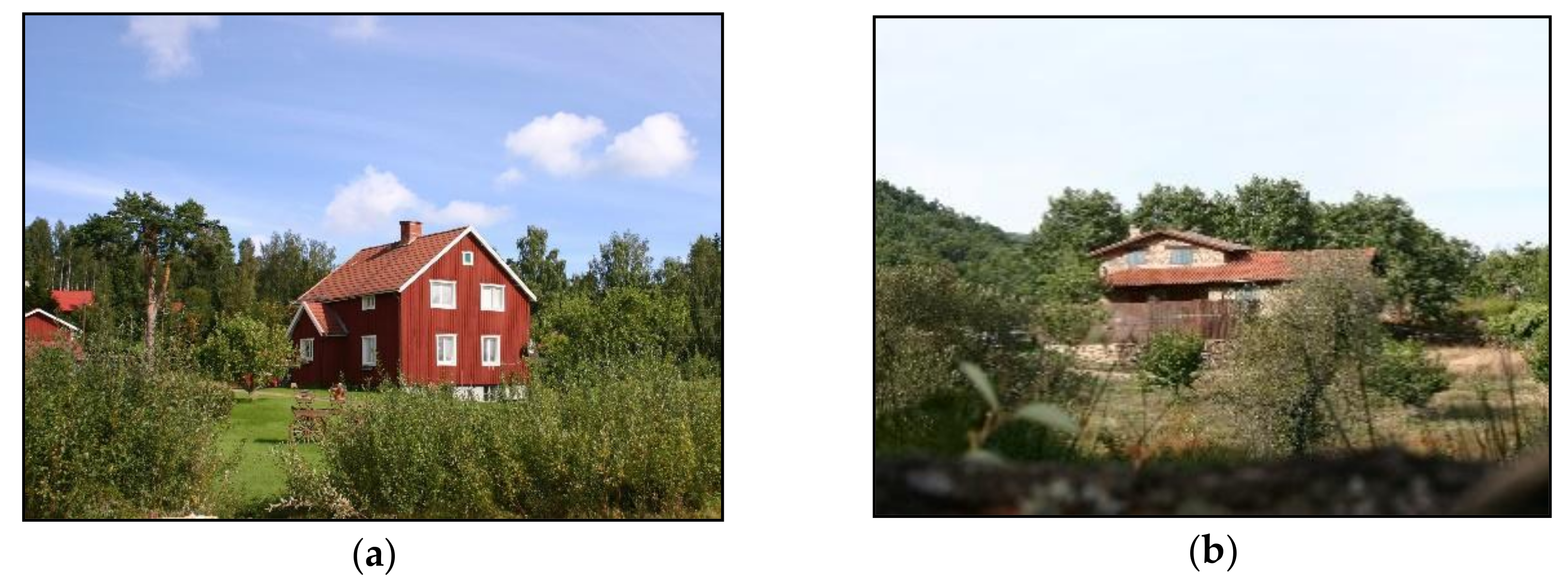
2.1.1. Spanish Pilot Area

• Physical environment:
Ambroz Valley enjoys a large natural diversity due to its wide range in altitude (400–2100 m). This provides optimum growing conditions for sustainable mature woodland, from high mountain and Atlantic woodland (Sweet chestnut (Castanea sativa), Pyrenean oak (Quercus pyrenaica), Holm oak (Ilex aquifolium), and yew (Taxus baccata)) to Mediterranean woodland, comprising of holm oak and old cork oak woods, areas under crops, and irrigated flat-bottomed valleys.
• Built environment:
The traditional mountain Mediterranean house represents the dominant architectural style in the pilot area [66]. The two main examples of this style are stoned and half-timbered homes, which are generally two storeys with a gabled roof [67]. Wood framing has traditionally been destined to the construction of the upper floors away from moisture and xylophages, using the lower floor’s masonry as the mainstay of the entire building. Framing is limed in some homes and is visible in others. New construction in rural areas tend to imitate these stiles, where the presence of stone and wood is generally accepted (Figure 2b).

2.1.2. Swedish Pilot Area

• Physical environment:
The vegetation of Norrland results from the dominance of mixed transitional woodlands giving way to taiga. These require a milder climate and soil that remains unfrozen for most of the year, always accompanied by undergrowth of grasses, ferns and moss. The dominant tree species are Sessile oak (Quercus petraea) on its northernmost boundary, and Norway spruce (Picea abies) at its southern limit, both intermixed with Scots pine (Pinus sylvestris) in the driest areas.
• Built environment:
The traditional Swedish rural home is also a two-storey building with occasional wood cladding on the façades. Several colors of façade are used, although white and red are the most common [68,69]. Falu (or falun) red is a dye that is still used to paint the walls a deep red, and is well-known in the countryside and rural areas for its use on wooden cottages and barns. The gabled roof of Swedish buildings presents a larger angle of inclination than Spanish houses due to extreme winter climatic conditions (Figure 2a).

2.1.3. Photo Capture and Case Selection

A field search of rural buildings in woodlands’ natural masses was conducted in both study areas. Potential cases from this fieldwork were selected for designing a public poll. The objective was to select buildings in the natural rural environments where the methodology of this research could be applied, and these were isolated rural houses with enough surrounding tree vegetation to allow digital modification in different height ratios.
Additional criteria were as follows:
  • Selection of the most representative vegetation and building combinations in both experimental areas, which complied with physical and built descriptions above.
  • Optimal visibility and access for image capturing. Dense urban cores were avoided.
  • Image capturing where the buildings filled some 30–50% of the image. This condition guaranteed full visibility of buildings as well as an acceptable amount of the surrounding landscape [10], allowing building scenes to be comparable with their most immediate setting (Figure 2a,b).
  • Buildings set in sky-sensitive locations: i.e., overshooting the skyline, or close to it.
  • Images captured in the sunny days of spring and early summer. Negative conditions such as rain, excessive cloudiness, fog, or midday sunlight were avoided [70,71].
Finally, each building and vegetation element inventoried was measured using the VERTEX Laser Hypsometer (height of building, height of adjacent vegetation). UTM coordinates were also taken for recording all cases in a Geographic Information System database.

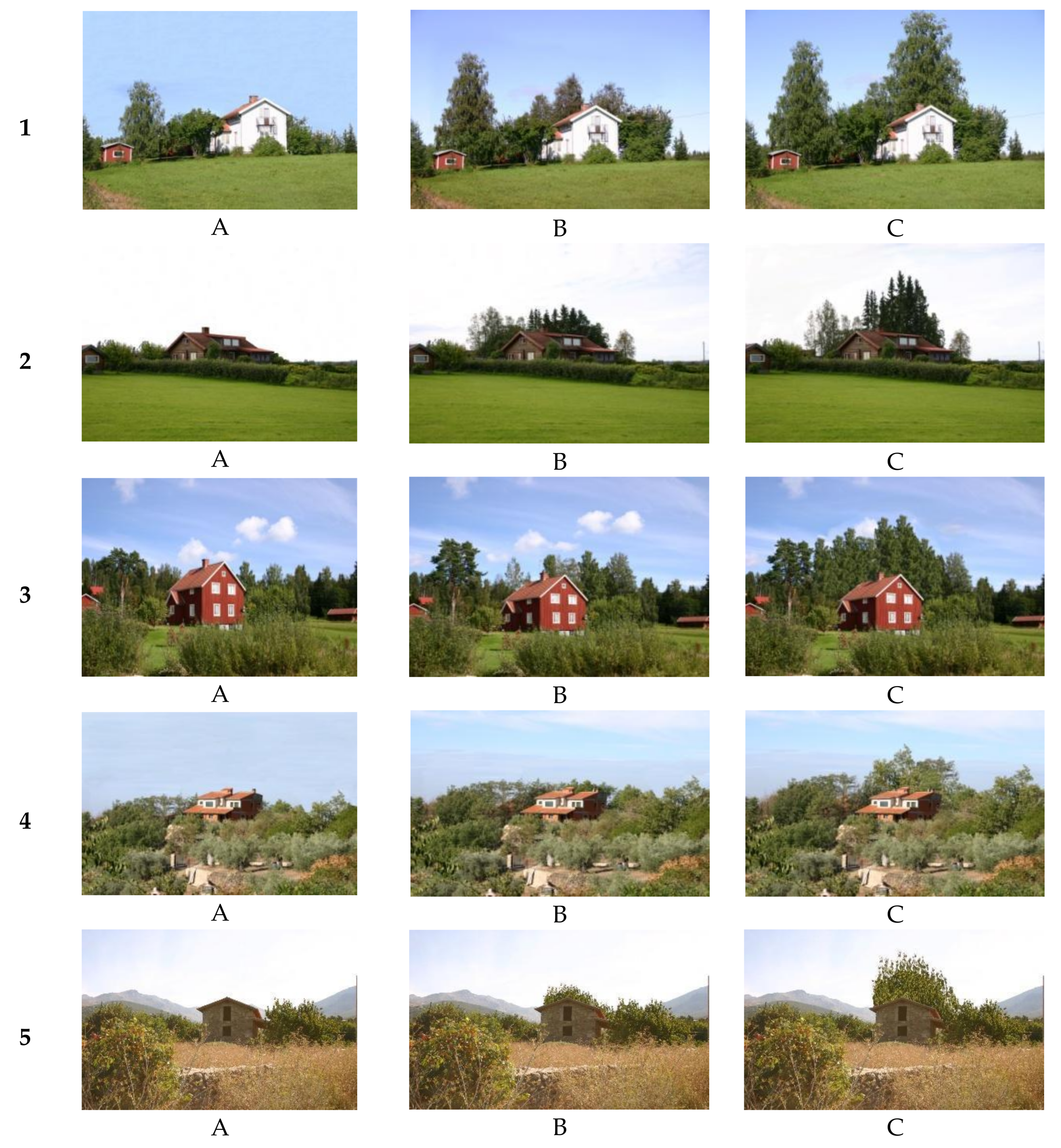
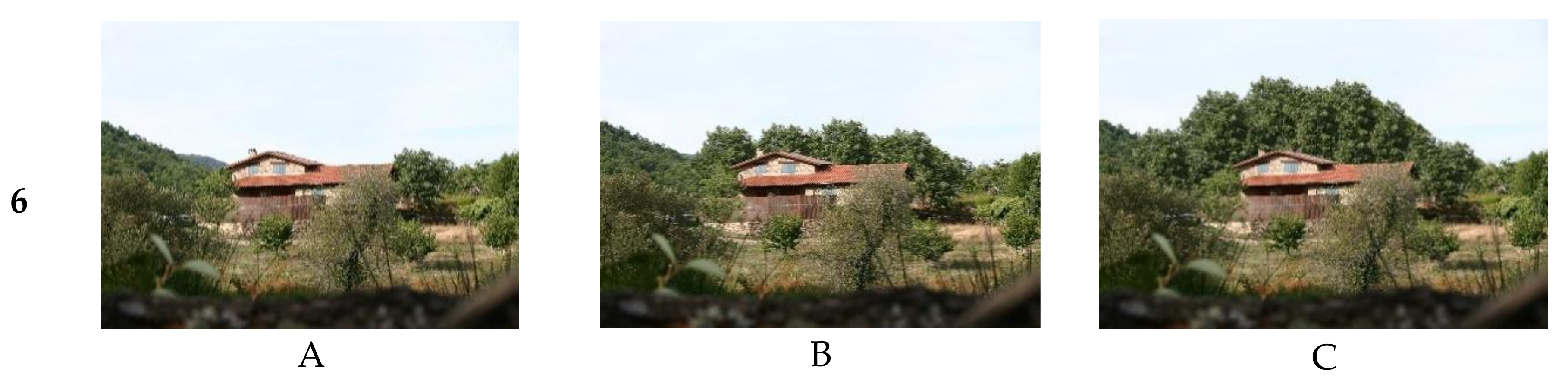
2.2. Visual Stimuli and Experimental Design of the Survey

Following the criteria laid down above, six scenarios were selected—three from Spain, and three from Sweden. This small sample size has been previously validated [53]. The rule of the golden section in regard to position of the horizon was ever complimented, since the horizon line was never placed in the lower third of the photograph (Figure 3) [72].
Three simulations were prepared from each original scenario by means of computer image treatment with Adobe Photoshop CS6® software [73]. Eighteen scenarios were obtained in total for evaluating visual stimuli (Figure 3), and they were modified by varying the height of the vegetation behind the building. The process never modified the building in the original picture, and the objective was to change the sharpness of the lines of the building against the skyline by changing the vegetation in the background. Changes in the colour of the sky, which is otherwise mutable by itself, have previously proved irrelevant [49] and were not performed.
The diverse vegetation vs. building height ranges of modification were laid out according to the Weber-Fechner Law (WFL) [56]. WFL describes the relationship between the magnitude of a physical stimulus and its perceived intensity, and is considered to be an important principle in psychophysics. According to this principle, the sensory system is able to notice differences as soon as the basic physical stimulus changes for more than a constant proportion of its actual magnitude [74,75,76].
An expert panel, constituted by landscape architects, planners, geographers, and ecologists, performed a prior evaluation of different height ratios according to the WFL. Ratios of about 50% were found to render significant changes, and the following were selected for the study on the basis of it (Figure 3):
1)
The vegetation did not exceed the height of the building’s eaves (A);
2)
The vegetation exceeded 0% to 50% of the building’s height (B);
3)
The vegetation exceeded 100% of the building’s height (C).

2.3. Measurement of the Height Ratio

Photographic resolution of the digital analysis fell into the range of 100 to 150 dpi. For pictures 10 × 15 in size, the number of pixels corresponding to these resolutions ranged from 393 × 591 to 591 × 886 pixels. These proportions were suitable for comparing the building with the surroundings and for appreciating details in the building [53]. The total height of buildings, and height ratios in relation to vegetation, were measured in terms of pixels by Adobe Photoshop CS6® [73].

2.4. Survey Procedure

A survey with the eighteen scenarios was performed for testing people’s preferences in relation to height­–ratio thresholds between the building and background vegetation (Figure 3). There was an adequate number of pictures per interviewee for keeping a correct visual attention until the end of the questionnaire, and for achieving consistent results [37,77,78,79,80]. Images were shown at random to the respondents in a face-to-face interview [81,82,83,84,85], and a member of the research group was always present during each poll [84].
Every interviewee was requested to complete a questionnaire, which consisted of two parts. The first part collected demographic and educational data from the participant (gender, age, country of origin, and educational background). The second part involved evaluation of the image sets, posing a question for each scenario, such as: “How would you rate the integration of the building in this scene?” Response options were arranged on a semantic scale according to the five-point Likert test, from very bad = 1, to very good = 5. A bipolar rating scale was selected from previous research, since semantic differential scales have already been successfully used to measure visual preferences [86]. Though scales with more intervals can be used [87], they have not been proven to help participants improve their evaluation [84].
Surveys were carried out in Spanish and in English.

2.5. Participants

Seventy-six individuals participated in the survey. Forty-four were students from Extremadura University of Spain and 32 from Gävle University of Sweden. The majority of Spanish participants (32) were less than 26 years old, of whom 25 were men and 17 were women. All students from Sweden were young in age, and 18 were men and 15 were women.

2.6. Statistical Analysis

Students’ valuations of each scenario was the dependent variable in this study. The mean value of this variable (onward: Rating Average (RA)) was calculated for each photograph, since its ordinal character from 1 to 5 allowed a continuous analysis of it [88]. Height–ratio between vegetation and buildings (HR) (cases A, B, or C, Figure 3), and the country of origin of the respondent (CO), were the independent variables (factors) considered in the analysis. Mean preference ratings were analyzed by using a two-way Analysis of Variance (ANOVA) factorial design: 2 (CO) × 3 (HR). The latter variable had a repeated measures analysis within subjects, and CO data comprised the analysis between subjects.
A posteriori pair-comparison of mean values per level of a factor (CO or HR) were performed by the Bonferroni test at a significance level of p ≤ 0.05 (post-hoc statistics). Two tests were made for comparing averages of scores per level of HR: one for Spanish respondents, and another for Swedish respondents. Additionally, post-hoc analysis was made comparing averages of scores per CO of the respondents by grouping responses according to their function at the HR level. Thus, three tests were performed in total—one per group of cases A, B, or C.
In statistics, the effect size is a measure of the strength of a phenomenon. The Cohen’s d index was also used in the statistical analysis of the results of the study, which estimated the effect size of the differences found between two levels of a factor (e.g., HR). Thus, we thought it may be able to indicate whether two scenarios were significantly different from each other, and by how much [89]. Moreover, this eventual effect can be numerically comparable with results from other studies by using the d index “d”. For Cohen’s d, an effect size up to 0.2 might be considered a “small” effect, around 0.5 a “medium” effect, and 0.8 to infinity a “large” effect; d > 0.2 is accepted as being a good threshold for distinguishing significant differences from non-significant ones in environmental visual assessments [90].
The sample size (n = 76) was assumed to be good enough for this study as it was at least able to detect effect sizes over 0.2 at significant thresholds of power analysis [(0.75 = 1 − β; β = 0.25); α = 0.05] [91].
All statistical analyses was carried out using the software SPSS 19® [92].

3. Results

3.1. Preliminary Results of ANOVA

The ANOVA analysis yielded a significant effect of CO on the dependent variable RA (Table 1). HR variation also had a significant influence on RA (responses from participants differed significantly in function of the HR level) (A to C, Figure 3). In addition, there was some interaction between HR and CO factors (HR was not assessed in the same levels by Spanish and Swedish respondents) (Table 2).

3.2. Rating of Images

The influence of HR on participants’ evaluations was also analyzed separately within each group of origin. Univariate analysis revealed significant differences for RA values in function of the HR level, and showed a strong effect size in both samples (Spanish group: F(2, 784) = 3.829, p < 0.022, d = 0.2; Swedish group: F(2, 568) = 47.899, p < 0.001, d = 0.82).

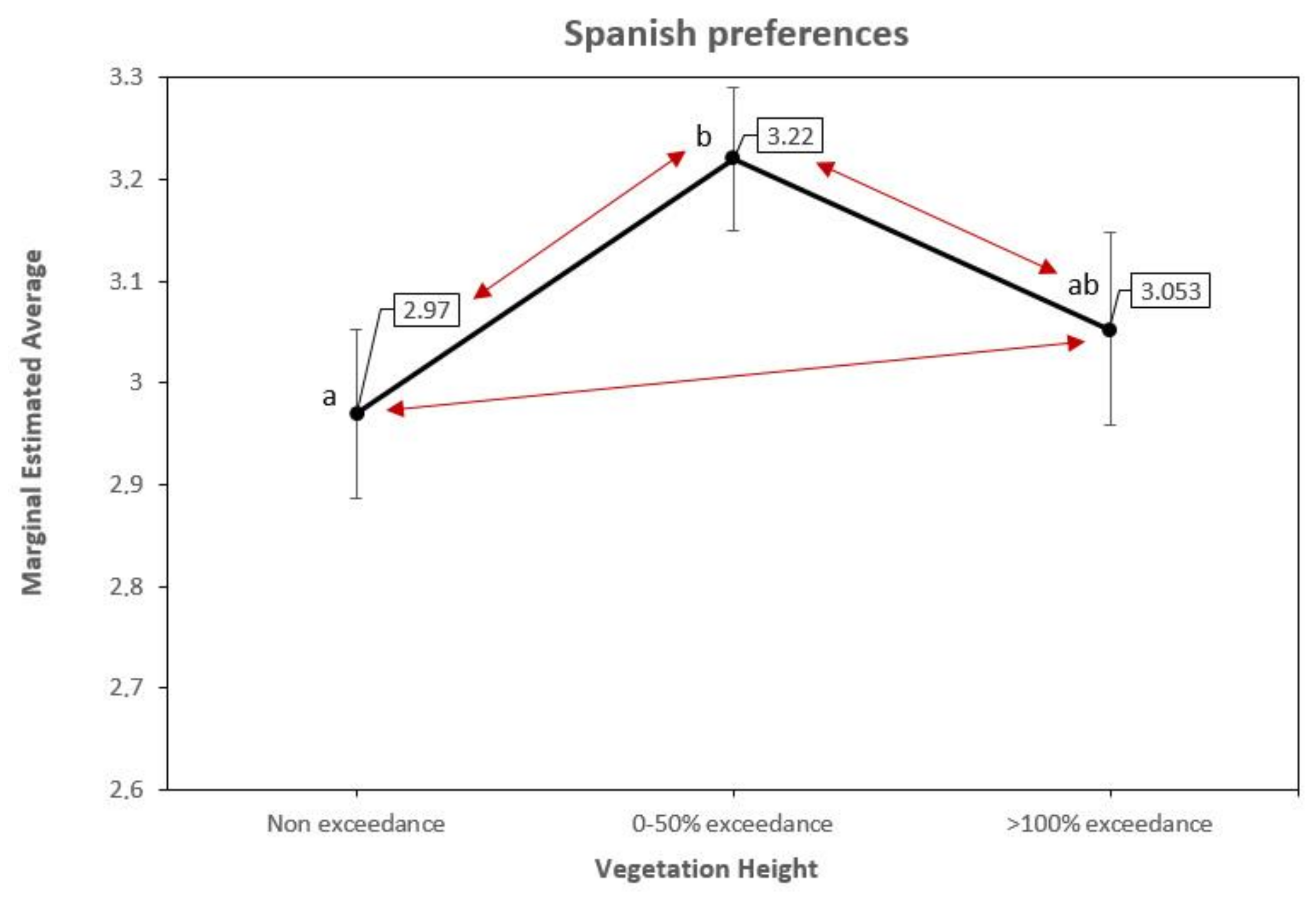
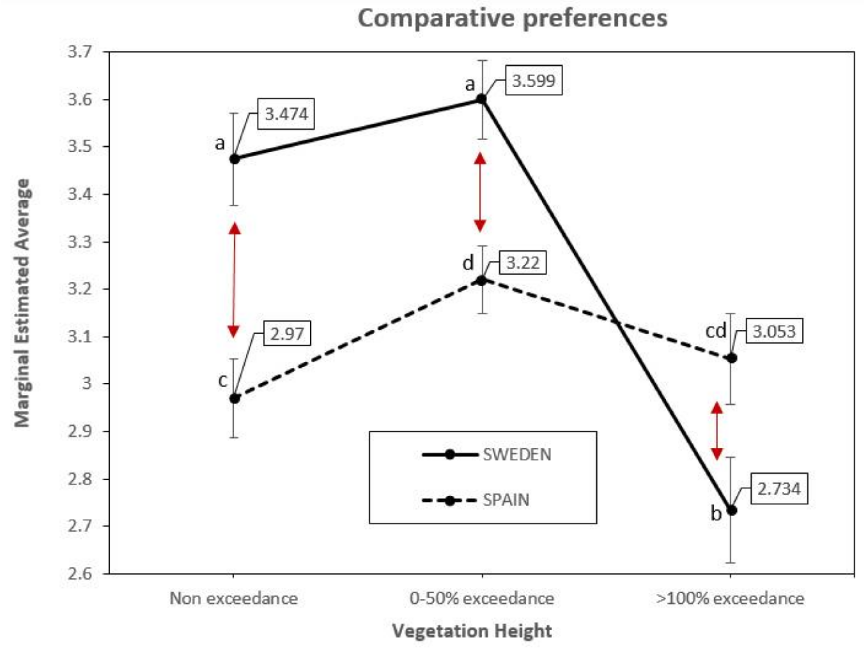
3.2.1. Spanish Preferences

Spanish participants considered on average that vegetation height exceeding 0 to 50% of building height (cases B of HR, Figure 3) provided the most integrated solution for the building, although the differences were statistically significant just in comparison to cases A. Images with vegetation exceeding over 100% of the building height (cases C of HR, Figure 3) were rated at the middle of the scale and did not render statistically significant differences in pairwise comparisons with cases A or B (Figure 4).

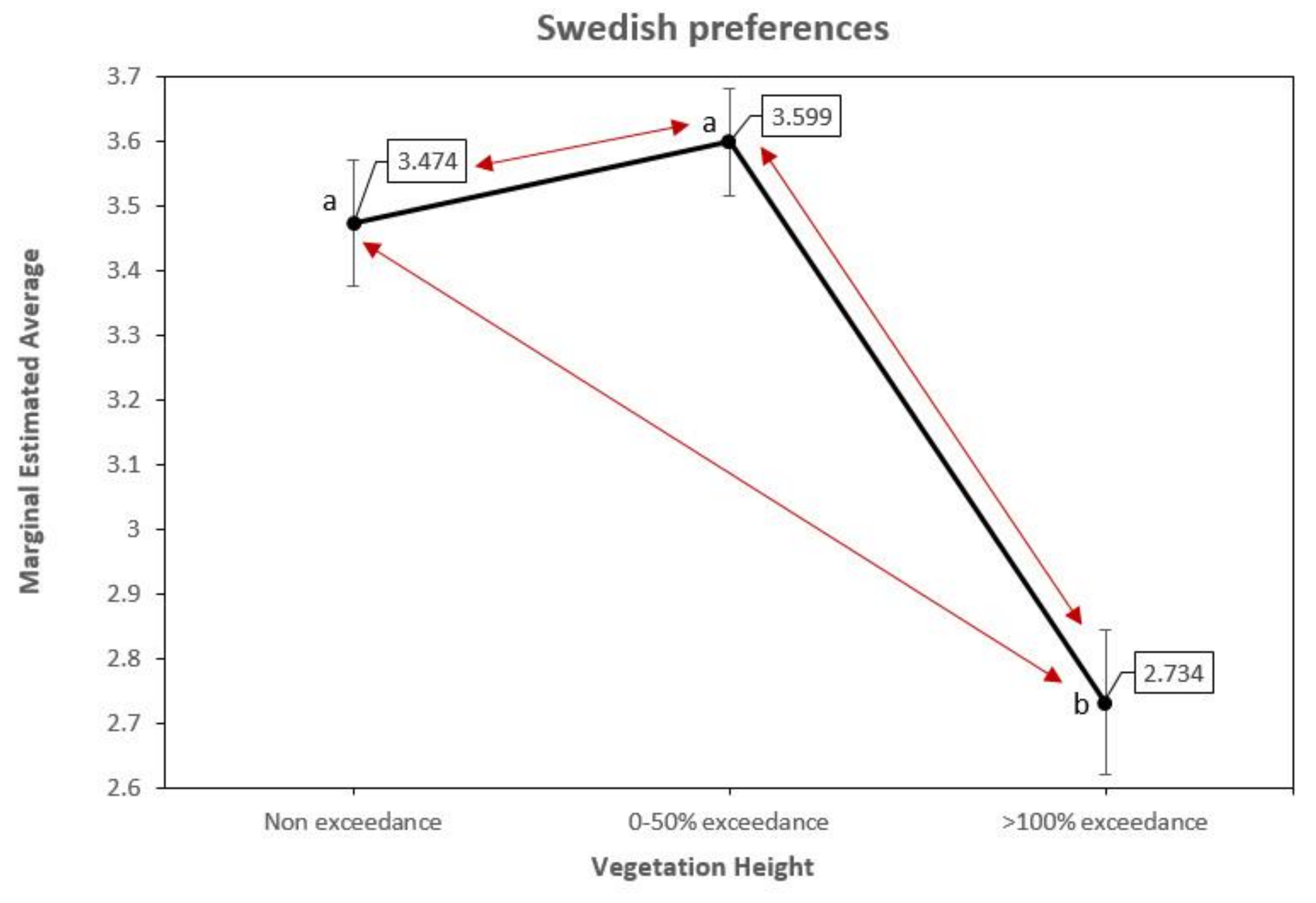
3.2.2. Swedish Preferences

RA values from Swedish participants displayed the same pattern observed among the Spaniards in regard to HR, with vegetation height exceeding 0 to 50% of the building height (cases B of HR, Figure 3) obtaining the highest score. Differences in this case were statistically significant just in comparison with cases C. Vegetation exceeding the building height over 100% (cases C of HR, Figure 3) displayed the lowest value on the rating scale, and the difference was statistically significant in pairwise comparisons with both cases A and B (Figure 5). Images A and B rendered comparable values in terms of statistics, though a weak upward trend to scoring better images B was appreciated.

3.3. Conjoint Analysis

Figure 6 shows a comparison between the RA values obtained in regard to CO among Swedish and Spanish participants. A significant interaction between CO and HR influencing the RA of the images was observed, and was of special significance for level C of HR variation. This effect was already found in the MANOVA analysis (Table 2).
Univariate analysis of the paired-cases comparison (Bonferroni test) was also performed, and revealed that both samples showed a similar pattern of responses up to level B of HR. Swedish RA values were, however, significantly higher than the Spanish ones (arrows in red, levels A and B). After reaching a maximum score at level B, both graphics went down at level C of HR, where the fall was worst for the Swedish group. The interaction found in the responses (Table 2) was therefore drawn at this level, indicating that the highest HR variation of vegetation was much worse among the Swedish participants than the Spaniards.

4. Discussion

4.1. Contribution of the Study

Growing awareness of the recreational potential of rural areas, coinciding with urban sprawl in the late 20th century and with the improvement of communications, has promoted recent human movement from urban to rural areas [93]. Consequently, many such areas in Europe are experiencing a disordered increase in the building of second-residence houses, which is quite often discordant with the local landscape [94,95]. Sweden and Spain share an intermediate place in terms of urban pressure on rural areas in comparison with countries from Central and Eastern Europe, and this circumstance made them suitable for the purpose of the investigation and justified their selection. On the other hand, their disparities in regard to their natural environment and human culture also made them appropriate for achieving the second objective of the study. No studies analyzing HR variations between buildings and their natural background elements or surroundings, and its effect on visual appeal, have been published to date. Therefore, the research approach of the present study can be considered original and innovative.
Although some authors question the validity of the photographic method for landscape assessment research and express doubts as to whether a photo can represent a complex scene or whether it can reliably evaluate attributes in the studio which are not perceptible via photos, such as sound, smell, and shades of color [96], most research vouches for the effectiveness of this technique [72,97,98,99]. In addition, infographic simulation starting from a photographed scene allows the comparison and evaluation of different scenarios [48,100,101,102,103,104,105]. Therefore, the experimental approach used in the present investigation can be defended as being valid and suitable.
Extreme levels of HR (A and C) rendered comparable statistical patterns of response among the Spanish participants, and intermediated levels (B) recorded the best RA values, also leading to significantly better results than the absence of vegetation in the background planes of the building. Such a solution seems, therefore, adequate for buildings overshooting the skyline in Spanish landscapes. On the other hand, images with vegetation exceeding more than 100% of the building height (C) obtained the worst RA value in the Swedish sample, which was significantly worse than those from both A and B image sets. This alternative should, therefore, be avoided for buildings overshooting the skyline in Swedish landscapes.
In spite of the interaction found between CO and HR variables, RA values followed in both CO samples showed a tendency to draw an inverted U-shaped curve reaching a maximum at intermediate HR values. Previous studies have found a significant correspondence between the degree of complexity of a facade in terms of materials or ornaments (independent factor) from absence to full coverage, and the preferences of the observers (dependent variable). All of them also registered a positive linear correspondence just up to a certain threshold, identifying too an inverted U-shaped correspondence [106,107]. A maximum threshold-point in the degree of variation of a factor, above which visual acceptance decreased in all cases, was ever found. In regard to height ratios, other studies suggested that the more contrasting the height of the building was with its surroundings, the worse was its visual acceptance. Using a sample of about 30 university students, Nasar and Stamps [56] investigated the visual effect of increasing building heights in relation to neighbor buildings in urban contexts, and concluded that an increment of 75% resulted in a sharp decrease of RA values of acceptance. Highly-contrasted scales in landscape planning have also been found unsuitable for a good visual integration, especially when the building height exceeded the horizon [52,53,59,108].
The present investigation contributes, therefore, to improving the knowledge on landscape planning by searching for a pattern or trend of visual responses to increments of a variable, which in this case is the height of the vegetation set in the background of a building. Like for other kinds of variables [56,107], an inverted U-shaped relationship between people’s preferences and vegetation height­–ratio increments was found. Vegetation may improve the integration of buildings into the landscape [49,50,52], and the present study provides, for the first time, a quantization of this effect which may be used fruitfully in planning activity.

4.2. Weaknesses of the Study

Current literature supports the sample size used in this study [109], and university students were also proven to be suitable subjects for the purposes of this kind of investigation [56,57,77,78,106,110,111]. Similar population samples were used successfully in prior studies [43,77,78,111], among others. Empirical tests suggest, in addition, that studies of environmental preferences using dependent variables of semantic scales require about 30 respondents for getting reliable findings (r > 0.90) [109]. However, sampling methods in social research is an ever-controversial issue, and caution must be taken when generalizing the results obtained with a particular sample to other population groups [112,113]. In this field of science, reliable statistical analysis of the dependent variable per crosses of social variables (such as gender, age, education background, and even profession), which guarantee a tolerated error of sampling, often implies a considerable increase of the sampling size per social variable, which also increases the costs of polling [112,113]. Taking all these issues into account, we consider that the findings of the present investigation are reliable enough to be accepted as a valid and useful approximation to the problem studied.

4.3. Future Research Recommendation

Differences found in the study between Swedish and Spanish participants may have been due to cultural and emotional factors, as suggested by other investigations in the field [61,62,63]. For example, tree species characteristic of each country may have played a role in the explanation of these differences, such as how the Swedish tended to reject images with vegetation strongly dominating the background of the building much more than the Spaniards. Further research is needed to confirm this point and perhaps identify other eventual causes.

4.4. Implication of the Results

The need to minimize visual impacts of buildings into the landscape was imposed by society’s growing awareness of environmental respect, and is a conservation that has arisen in recent years [48,114,115]. However, legislation is very vague in terms of the visual integration of buildings into the environment. Criteria proposed by present planning rules are not necessarily the most appropriate, and there is seldom an efficient follow-up of rule compliance.
One option for integrating buildings into the rural landscape is to analyze their visual relationship with the setting and to highlight vegetation as the main element of it [52,54,116,117], and the results from the present investigation represent a step forward in the evaluation of the vegetation scale. This may be applied to buildings from rural settings to minimize their scale impact, and could help planners and designers in figuring out the optimal design. The use of vegetation screens in the background that do not exceed one-half of the height of the building facilitates a simple and quantified criterion that could be used by engineers and architects for improving the integration of buildings into the rural landscape without increasing costs, and this may easily be integrated into the specific building regulations of Sweden and Spain in the future.

5. Conclusions

In summary, our study of the variations of height ratios between buildings and background vegetation by using digital image processing of selected photographs and public preference surveys conducted in Sweden and Spain has identified an optimal threshold value for visual acceptance of around 50%. This threshold provides a quantitative criterion for improving the integration of buildings into the rural landscape that may be incorporated into the regulations on edification in rural settings from both countries. However, some significant differences between Swedish and Spanish observers were recorded in regard to the acceptance of some extreme scenarios. Cultural and emotional factors might account for them, and new investigations may identify additional elements for further improvement.

Author Contributions

Formal analysis, J.G.-V., M.J.M.-P., J.H.-B. and L.G.-M.; Funding acquisition, J.H.-B. and L.G.-M.; Investigation, J.G.-V., M.J.M.-P., J.H.-B. and L.G.-M.; Methodology, J.G.-V., M.J.M.-P., J.H.-B. and L.G.-M.; Project Administration, J.H.-B.; Supervision, M.J.M.-P., J.H.-B. and L.G.-M.; Writing—original draft, J.G.-V.; Writing—review & editing, J.G.-V., M.J.M.-P., J.H.-B. and L.G.-M.

Funding

This article has been funded by the Ministry of Science and Innovation, (Proyect BIA2007-61166) and the government of Extremadura (Ref. GR18176).

Acknowledgments

Publication of this article has been possible thanks to the funding Ministry of Science and Innovation, Plan Nacional de I+D+I project reference BIA2007-61166, as well as the funding of the Government of Extremadura and the European Regional Development Fund (ERDF), reference GR18176.

Conflicts of Interest

The authors declare no conflict of interest.

References

  1. Sanders, R.A. Urban vegetation impacts on the urban hydrology of Dayton Ohio. Urban Ecol. 1986, 9, 361–376. [Google Scholar] [CrossRef]
  2. Akbari, H.; Pomerantz, M.; Taha, H. Cool surfaces and shade trees to reduce energy use and improve air quality in urban areas. Sol. Energy 2001, 70, 295–310. [Google Scholar] [CrossRef]
  3. Nowak, D.J.; Crane, D.E. Carbon storage and sequestration by urban trees in the USA. Environ. Pollut. 2002, 116, 381–389. [Google Scholar] [CrossRef]
  4. Dimoudi, A.; Nikolopoulo, M. Vegetation in the urban environment, microclimatic analysis and benefits. Energy Build. 2003, 35, 69–76. [Google Scholar] [CrossRef]
  5. Escobedo, F.J.; Kroeger, T.; Wagner, J.E. Urban forests and pollution mitigation: Analyzing ecosystem services and disservices. Environ. Pollut. 2011, 159, 2078–2087. [Google Scholar] [CrossRef] [PubMed]
  6. Roy, S.; Byrne, J.; Pickering, C. A systematic quantitative review of urban tree benefits, costs, and assessment methods across cities in different climatic zones. Urban For. Urban Green. 2012, 11, 351–363. [Google Scholar] [CrossRef]
  7. Tzilkowski, W.M.; Wakeley, J.S.; Morris, L.J. Relative use of municipal street trees by birds during summer in state college. Pennsylvania. Urban Ecol. 1986, 9, 387–398. [Google Scholar] [CrossRef]
  8. Savard, J.P.L.; Clergeau, P.; Mennechez, G. Biodiversity concepts and urban ecosystems. Landsc. Urban Plan. 2000, 48, 131–142. [Google Scholar] [CrossRef]
  9. Davies, Z.G.; Fuller, R.A.; Loram, A.; Irvine, K.N.; Sims, V.; Gast, K.J. A national scale inventory of resource provision for biodiversity within domestic gardens. Biol. Conserv. 2009, 142, 761–771. [Google Scholar] [CrossRef] [Green Version]
  10. Brush, R.G.; Williamson, D.N.; Fabos, J.G.Y. Visual screening potential of forest vegetation. Urban Ecol. 1979, 4, 207–216. [Google Scholar] [CrossRef]
  11. Wherret, J.R. Nature Landscape Scenic Preference: Techniques for Evaluation and Simulation. Ph.D. Thesis, Robert Gordon University, Aberdeen, UK, 1998. [Google Scholar]
  12. Bishop, I.D.; Wherret, J.R.; Miller, D.R. Using image depth variables as predictors of visually quality. Environ. Plan. B 2000, 865–875. [Google Scholar] [CrossRef]
  13. Ulrich, R.S. Human responses to vegetation and landscapes. Landsc. Urban Plan. 1986, 13, 29–44. [Google Scholar] [CrossRef]
  14. Anderson, L.M.; Cordell, H.K. Influence of trees on residential property values in Athens, Georgia (USA), A survey based on actual sales prices. Landsc. Urban Plan. 1988, 15, 153–164. [Google Scholar] [CrossRef]
  15. Dwyer, J.; McPherson, E.; Schroeder, H.; Rowntree, R. Assessing the benefits and costs of the urban forest. J. Arboric. 1992, 18, 227–234. [Google Scholar]
  16. Velarde, M.D.; Fry, G.; Tveit, M. Health effects of viewing landscapes–Landscape types in environmental psychology. Urban For. Urban Green. 2007, 6, 199–212. [Google Scholar] [CrossRef]
  17. Nilsson, K.; Sangster, M.; Gallis, C.; Hartig, T.; De Vries, S.; Seeland, K.; Schipperijn, J. Forest, Trees and Human Health; Springer: Dordrecht, The Netherlands, 2011. [Google Scholar]
  18. Schroeder, H.W.; Cannon, W.N. The aesthetic contribution of trees to residential streets in Ohio towns. J. Arboric. 1983, 9, 237–243. [Google Scholar]
  19. Serpa, A.; Muhar, A. Effects of plant size, texture and colour on spatial perception in public green areas—A cross-cultural study. Landsc. Urban Plan. 1996, 36, 19–25. [Google Scholar] [CrossRef]
  20. Kuo, F.E. The role of arboriculture in a healthy social ecology. J. Arboric. 2003, 29, 148–155. [Google Scholar]
  21. Todorova, A.; Asakawa, S.; Aikoh, T. Preferences for and attitudes towards street flowers and trees in Sapporo, Japan. Landsc. Urban Plan. 2004, 69, 403–416. [Google Scholar] [CrossRef]
  22. Acar, C.; Acar, H.; Eroglu, E. Evaluation of ornamental plant resources to urban biodiversity and cultural changing, A case study of residential landscapes in Trabzon city (Turkey). Build. Environ. 2007, 42, 218–229. [Google Scholar] [CrossRef]
  23. Holm, D. Thermal improvement by means of leaf-cover on external walls—A simultion model. Energy Build. 1989, 14, 19–30. [Google Scholar] [CrossRef]
  24. Krishan, A. Climate Responsive Architecture, a Design Handbook for Energy Efficient Buildings; Tata McGraw-Hill Education: Noida, India, 2001. [Google Scholar]
  25. Gómez-Muñoz, V.M.; Porta-Gándara, M.A.; Fernández, J.L. Effect of tree shades in urban planning in hot-arid climatic regions. Landsc. Urban Plan. 2010, 94, 149–157. [Google Scholar] [CrossRef]
  26. Heisler, G. Energy savings with trees. J. Aboric. 1986, 12, 113–125. [Google Scholar]
  27. Zube, E.H. Themes in Landscape Assessment Theory. Landsc. J. 1984, 3, 104–110. [Google Scholar] [CrossRef]
  28. Arthur, L.M.; Daniel, T.C.; Baster, R.S. Scenic Assessment: An overview. Landsc. Plan. 1997, 4, 109–129. [Google Scholar] [CrossRef]
  29. Coeterier, J.F. Dominant attributes in the perception and evaluation of the Dutch landscape. Landsc. Urban Plan. 1996, 34, 27–44. [Google Scholar] [CrossRef]
  30. Jeong, J.S.; García, L.; Hernández, J. A site planning approach for rural buildings into a landscape using a spatial multi-criteria decision analysis methodology. Land Use Policy 2013, 32, 108–118. [Google Scholar] [CrossRef]
  31. Otero, I.; Casemeiro, M.A.; Ezquerra, A.; Esparcia, P. Landscape evaluation: Comparison of evaluation methods in a region of Spain. J. Environ. Manag. 2007, 85, 204–214. [Google Scholar] [CrossRef] [PubMed]
  32. Daniel, T.C. Whither scenic beauty? Visual landscape quality assessment in the 21st century. Landsc. Urban Plan. 2001, 54, 267–281. [Google Scholar] [CrossRef]
  33. Tassinari, P.; Torreggiani, D. Visual Impact Assessment Methodologies for Rural Building Desgin. CIGR 2006, 8, 1–16. Available online: http://www.cigrjournal.org/index.php/Ejounral/article/view/620 (accessed on 24 July 2018).
  34. Swanwich, C. Society’s attitude to and preferences for land and landscape. Land Use Policy 2009, 26, 62–75. [Google Scholar] [CrossRef]
  35. Kaplan, R.; Kaplan, S.L. The visual environment: Public participation in design and planning. J. Soc. Issues 1989, 41, 59–86. [Google Scholar] [CrossRef]
  36. Svobodova, K.; Vojar, J.; Sklenicka, P.; Filova, L. Presentation matters: Causes of differences in preferences for Agricultural landscapes displayed via photographs and videos. Space Cult. 2017, 21, 259–273. [Google Scholar] [CrossRef]
  37. Purcell, T. Experiencing American and Australian high and popular style houses. Environ. Behav. 1995, 27, 771–800. [Google Scholar] [CrossRef]
  38. Samavatekbatan, A.; Gholami, S.; Karimimoshaver, M. Assessing the visual impact of physical features of tall buildings: Height, top, color. Environ. Impact Assess. 2016, 57, 53–62. [Google Scholar] [CrossRef]
  39. Wang, W.; Wang, W.; Namgung, M. Linking people’s perceptions and physical components of sidewalk environments: An application of rough sets theory. Environ. Plan. B 2010, 37, 234–247. [Google Scholar] [CrossRef]
  40. Cañas, I.; Ayuga, E.; Ayuga, F. A contribution to the assessment of scenic quality of landscapes based on preferences expressed by the public. Land Use Policy 2009, 26, 1173–1181. [Google Scholar] [CrossRef]
  41. Dupont, L.; Ooms, K.; Antrop, M.; Eetvelde, V. Comparing saliency maps and eye-tracking forms maps: The potential use in visual impact assessment base on landscape photographs. Landsc. Urban Plan. 2016, 148, 17–26. [Google Scholar] [CrossRef]
  42. Jeong, J.S.; García, L.; Hernández, J. Integration Building into a rural landscape using a multi-criteria apatial decision analysis in GIS-enabled web environment. Biosyst. Eng. 2012, 112, 82–92. [Google Scholar] [CrossRef]
  43. Ramírez, A.; Ayuga, E.; Gallego, E.; Fuentes, J.M.; García, A.I. A simplified model to assess landscape quality from rural roads in Spain. Agric. Ecosyst. Environ. 2011, 142, 205–212. [Google Scholar] [CrossRef]
  44. Stamps, A.E., III. A paradigm for distinguishing significant from non-significant visual impacts: Theory, implementation, case histories. Environ. Impact Assess. 1997, 17, 249–293. [Google Scholar] [CrossRef]
  45. Wood, G. Thresholds and criteria for evaluating and communication impact significance in environmental statements: See no evil, hear no evil, speak no evil? Environ. Impact Assess. 2008, 28, 22–38. [Google Scholar] [CrossRef]
  46. Sheppard, S.R.J. Visual Simulation: A User’s Guide for Architects, Engineers and Planner; Van Nostrand Reinhold: New York, NY, USA, 1989. [Google Scholar]
  47. Gómez-Orea, D. Evaluación del Impacto Ambiental; Ed Agrícola Española: Madrid, Spain, 1992. [Google Scholar]
  48. Garrido, J.; Montero, M.J.; Hernández, J.; García, L. Use of video and 3D scenario visualization to rate vegetation screens for integrating buildings into the landscape. Sustainability 2017, 9, 1102. [Google Scholar]
  49. García, L.; Montero, M.J.; Hernández, J.; López, S. Analysis of lines and forms in buildings to rural landscape integration. Span. J. Agric. Res. 2010, 8, 833–847. [Google Scholar] [CrossRef]
  50. Smardon, R.C. Perception and aesthetics of the urban environment: Review of the role of vegetation. Landsc. Urban Plan. 1988, 15, 85–106. [Google Scholar] [CrossRef]
  51. Español, I. Las Obras Públicas en el Paisaje: Guía para el Análisis y Evaluación del Impacto Ambiental en el Paisaje; Centro de Estudios de Técnicas Aplicadas: Madrid, Spain, 1998. [Google Scholar]
  52. Hernández-Blanco, J.; García-Moruno, L.; Morán, J.; Juan, A.; Ayuga, F. Estimating visual perception of rural landscapes using GIS: The influence of vegetation. J. Food Agric. Environ. 2003, 1, 139–141. [Google Scholar]
  53. Montero, M.J.; García-Moruno, L.; López-Casares, S.; Hernández Blanco, J. Visual impact assessment of color and scale of buildings on the rural landscape. Environ. Eng. Manag. J. 2016, 15, 1537–1550. [Google Scholar]
  54. Hernández, J.; García, L.; Ayuga, F. Assessment of the visual impact made on the landscape by new buildings: A methodology for site selection. Landsc. Urban Plan. 2004, 68, 15–28. [Google Scholar] [CrossRef]
  55. Zonneveld, I.S.; Forman, R.T.T. Changing Landscapes: An Ecological Perspective; Springer: New York, NY, USA, 1990. [Google Scholar]
  56. Nasar, J.L.; Stamps, A.E., III. Infill McMansions: Style and the psychophysics of size. J. Environ. Psychol. 2009, 29, 110–123. [Google Scholar] [CrossRef]
  57. Li, L.; Homma, R.; Kazuhisa, I. Preferences for a lake landscape: Effects of building height and lake width. Environ. Impact Assess. 2018, 70, 22–33. [Google Scholar]
  58. Grossberg, S.; Pessoa, L. Texture segregation, surface representation and figure ground separation. Vision Res. 1998, 38, 2657–2684. [Google Scholar] [CrossRef]
  59. Krause, C.L. Our visual landscape managing the landscape under special consideration of visual aspects. Landsc. Urban Plan. 2001, 54, 239–254. [Google Scholar] [CrossRef]
  60. Henderson, S.P.B.; Perkins, N.H.; Nelischer, M. Residential lawn alternatives: A study of their distribution, form and structure. Landsc. Urban Plan. 1998, 42, 135–145. [Google Scholar] [CrossRef]
  61. Berlyne, D.E. Aesthetics and Psychobiology; Appleton-Century-Crofts: New York, NY, USA, 1972. [Google Scholar]
  62. Nasar, J.L. Visual preferences in urban street scenes. A cross-cultural comparison between Japan and the United States. J. Cross Cult. Psychol. 1984, 15, 79–93. [Google Scholar] [CrossRef]
  63. Priego, C.; Breuste, J.; Rojas, J. Espacios naturales en zonas urbanas. Analisis comparado de la ciudad alemana de Halle y las chilenas de San Pedro de la Paz y Talcahuano. Rev. Int. Sociol. 2010, 68, 199–224. [Google Scholar] [CrossRef]
  64. Jeong, J.S.; Montero-Parejo, M.J.; García-Moruno, L.; Hernández-Blanco, J. The visual evaluation of rural areas: A methodological approach for the spatial planning and color design of scattered second homes with an example in Hervás, Western Spain. Land Use Policy 2015, 46, 330–340. [Google Scholar] [CrossRef]
  65. Nilsson, B.; Lundgren, A.S. Logics of rurality: Political rhetoric about the Swedish North. J. Rural Stud. 2015, 37, 85–95. [Google Scholar] [CrossRef]
  66. Rubio Masa, J.C. Arquitectura Popular del Extremadura (Vernacular Architecture of Extremadura Region (Spain); Cuadernos Populares n° 8. Consejería de Educación y Cultura; Dirección General de Acción Cultural, Junta de Extremadura: Mérida, Spain, 1985. [Google Scholar]
  67. Maldonado Ramos, L.; Rivera Gámez, D. El Entramado de Madera como Arquetipo Constructivo: De la Arquitectura Tradicional a los Sistemas Modernos. (The Wooden Structures as an Archetype of Construction: From Traditional to Modern Architecture). Actas del IV Congreso Nacional de Historia de la Construcción, Cádiz, 27–29 Enero 2005. Huerta, S., Editor. Madrid: I. Juan de Herrera, SEdHC, Arquitectos de Cádiz, COAAT. Available online: http://www.sedhc.es/biblioteca/paper.php?id_p=839 (accessed on 19 July 2016).
  68. Wingård, C. Renovergingsrad för Äldre hus i Tanum; Rio Kulturkooperativ: Munkedal, Sweden, 2013. [Google Scholar]
  69. Björk, C.; Nordling, L.; Reppen, L. Syggdes Villan Svensk Villaarkitektur fran 1890 till 2010; Svensk Byggtjänst, Göteborgstryckeriet: Mölndal, Sweden, 2015. [Google Scholar]
  70. Bishop, I.D. Determination of thresholds of visual impact: The case of wind turbines. Environ. Plan. B 2002, 29, 707–718. [Google Scholar] [CrossRef]
  71. Grèt-Regemy, A.; Bishop, I.D.; Bebi, P. Predicting the scenic beauty value of mapped landscape changes in a mountainous region through the use of GIS. Environ. Plan. B 2007, 34, 50–67. [Google Scholar] [CrossRef]
  72. Svobodova, K.; Sklenicka, P.; Molnarova, K.; Vojar, J. Does the Composition of Landscape Photographs Affect Visual Preferences? The Rule of the Golden Section and the Position of the Horizon. J. Environ. Psychol. 2014, 38, 143–152. [Google Scholar] [CrossRef]
  73. Córdoba, E.; Córdoba, C.; González, C. Photoshop Cs6. Curso Avanzado; Ed.RA-MA: Madrid, Spain, 2013; Available online: https://www.agapea.com/Enrique-Cordoba-Moreno/PHOTOSHOP-CS6-CURSO-AVANZADO-9788499642543-i.htm (accessed on 24 July 2018).
  74. Weber, E.H. De Pulsu, Resorptione, Auditu Et Tactu. Annotationes Anatomicae et Physiologicae; Koehler: Leipzig, Germany, 1834. [Google Scholar]
  75. Varela, M. Évaluation Pseudo–Subjective de la Qualité d’un Flux Multimédia. Ph.D. Thesis, University of Rennes 1, Rennes, France, 2007. [Google Scholar]
  76. Reichl, P.; Egger, S.; Schatz, R.; D’Alconzo, A. The logarithmic nature of QoE and the Role of the Weber-Fechner Law in QoE assessment. In Proceedings of the 2010 IEEE International Conference on Communications, Cape Town, South Africa, 23–27 May 2010. [Google Scholar]
  77. Stamps, A.E., III. Physical determinants of preferences for residential facades. Environ. Behav. 1999, 31, 723–751. [Google Scholar] [CrossRef]
  78. Akalin, A.; Yildirim, K.; Wilson, C.; Kilicoglu, O. Architecture and engineering students’ evaluations of house façades: Preference, complexity and impressiveness. J. Environ. Psychol. 2009, 29, 124–132. [Google Scholar] [CrossRef]
  79. Hernández, J.; López-Casares, S.; Montero, M.J. Análisis metodológico de la relación entre envolvente y urbanización exterior en construcciones rurales para la mejora de la integración paisajística. Inf. Constr. 2013, 65, 497–508. [Google Scholar] [CrossRef] [Green Version]
  80. Stamps, A.E., III. Advances in visual diversity and entropy. Environ. Plan. B 2003, 30, 449–463. [Google Scholar] [CrossRef]
  81. Pinto-Correia, T.; Barroso, F.; Surová, D.; Menezes, H. The fuzziness of Montado landscapes: Progress in assessing user preferences through photo-based surveys. Agrofor. Syst. 2011, 82, 209–224. [Google Scholar] [CrossRef]
  82. Arriaza, M.; Cañas-Ortega, J.F.; Cañas-Madueño, J.A.; Ruiz-Avilés, P. Assessing the visual quality of rural landscapes. Landsc. Urban Plan. 2004, 69, 115–125. [Google Scholar] [CrossRef]
  83. Paar, P. Landscape visualizations: Applications and requirements of 3D visualization software for environmental planning. Comput. Environ. Urban Syst. 2006, 30, 815–839. [Google Scholar] [CrossRef]
  84. Lange, E.; Hehl-Lange, S.; Brewer, M.J. Scenario-visualization for the assessment of perceived green space qualities at the urban-rural fringe. J. Environ. Manag. 2008, 89, 245–256. [Google Scholar] [CrossRef] [PubMed]
  85. Christopher, J.P.; Christopher, M.R.; Brett, A.B.; Hayden, L. Identifying strengths and weaknesses of landscape visualization for effective communication of future alternatives. Landsc. Urban Plan. 2011, 100, 231–241. [Google Scholar]
  86. Nasar, J.L. Adult viewers’ preferences in residential scenes: A study of the relationship of the environmental attributes to preference. Environ. Behav. 1983, 15, 589–614. [Google Scholar] [CrossRef]
  87. Roth, M. Validating the use of Internet survey techniques in visual landscape assessment-An empirical study from Germany. Landsc. Urban Plan. 2006, 78, 179–192. [Google Scholar] [CrossRef]
  88. Kendrick, J. Social Statistics: An Introduction to Using SPSS, 2nd ed.; Allyn and Bacon: Boston, MA, USA, 2005. [Google Scholar]
  89. Cohen, J. Statistical Power Analysis for the Behavioral Sciences, 2nd ed.; Lawrence Erlbaum Associates Publishers (LEA): New York, NY, USA, 1988. [Google Scholar]
  90. Stamps, A.E., III; Nasar, J.L. Design review and public preferences: Effects of geographical location, public consensus, sensation seeking, and architectural styles. J. Environ. Psychol. 1997, 17, 11–32. [Google Scholar] [CrossRef]
  91. Rosenthal, R.; Rosnow, R.L. Essentials of Behavioral Research: Methods and Data Analysis, 2nd ed.; McGraw Hill: New York, NY, USA, 1991. [Google Scholar]
  92. Norusis, M. IBM SPSS Statistics 19 Guide to Data Analysis: International Edition; Pearson: London, UK, 2012. [Google Scholar]
  93. Dwyer, J.F.; Childs, G.M. Movement of people across the landscape; a blurring of distinctions between area, interests, and issues affecting natural resource management. Landsc. Urban Plan. 2004, 69, 153–164. [Google Scholar] [CrossRef]
  94. Gallent, N.; Tewdwr-Jones, M. Rural Second Homes in Europe: Examining Housing Supply and Planning Control; Ashgate: Aldershot/Hampshire, UK, 2000. [Google Scholar]
  95. Ehrlich, M.V.; Hilber Cristian, A.L.; Schöni, O. Institutional setting and urban sprawl: Evidence from Europe. J. Hous. Econ. 2018. [Google Scholar] [CrossRef]
  96. Palmer, J.F.; Hoffman, R.E. Rating reliability and representation validity in scenic landscape assessments. Landsc. Urban Plan. 2001, 54, 149–161. [Google Scholar] [CrossRef]
  97. Shafer, E.L.; Brush, R.O. How to measure preferences for photographs of natural landscapes? Landsc. Plan. 1977, 4, 237–256. [Google Scholar] [CrossRef]
  98. Stewart, T.R.; Middleton, P.; Downton, M.; Ely, D. Judgments of photographs vs. field observations in studies of perception and judgment of the visual environment. J. Environ. Psychol. 1984, 4, 283–302. [Google Scholar] [CrossRef]
  99. Hull, R.B.; Stewart, W.P. Validity of photo-based scenic beauty judgments. J. Environ. Psychol. 1992, 12, 101–114. [Google Scholar] [CrossRef]
  100. Bishop, I.D.; Leahy, P.N.A. Assessing the Visual Impact of Development Proposals: The Validity of Computer Simulations. Landsc. J. 1989, 8, 92–100. [Google Scholar] [CrossRef]
  101. Tress, B.; Tress, G. Scenario visualization for participatory landscape planning-a study from Denmark. Landsc. Urban Plan. 2003, 64, 161–178. [Google Scholar] [CrossRef]
  102. Dockerty, T.; Lovett, A.; Appleton, K.; Bone, A.; Sünnenberg, G. Developing scenarios and visualizations to illustrate potential policy and climatic influences on future agricultural landscapes. Agric. Ecosyst. Environ. 2006, 114, 103–120. [Google Scholar] [CrossRef]
  103. García, L.; Hernández, J.; Ayuga, F. Analysis of the materials and exterior texture of agro-industrial buildings: A photo-analytical approach to landscape integration. Landsc. Urban Plan. 2006, 74, 110–124. [Google Scholar] [CrossRef]
  104. Ghadirian, P.; Bishop, I.D. Integration of augmented reality and GIS: A new approach to realistic landscape visualization. Landsc. Urban Plan. 2008, 86, 226–232. [Google Scholar] [CrossRef]
  105. Barroso, F.L.; Pinto-Correia, T.; Ramos, I.L.; Surová, D.; Menezes, H. Dealing with landscape fuzziness in user preference studies: Photo-based questionnaires in the Mediterranean context. Landsc. Urban Plan. 2012, 104, 329–342. [Google Scholar] [CrossRef] [Green Version]
  106. Wohlwill, J.F. Amount of stimulus exploration and preference as differential functions of stimulus complexity. Percept. Psychophys. 1968, 14, 307–312. [Google Scholar] [CrossRef]
  107. Wohlwill, J.F. Children’s responses to meaningful pictures varying in diversity: Exploration time vs. preference. J. Exp. Child Psychol. 1975, 20, 341–351. [Google Scholar] [CrossRef]
  108. Zacharias, J. Preferences for view corridors through the urban environment. Landsc. Urban Plan. 1999, 43, 217–225. [Google Scholar] [CrossRef]
  109. Stamps, A.E., III. Bootstrap investigation of respondent sample size for environmental preference’. Percent. Mot. Skills 1992, 75, 220–222. [Google Scholar] [CrossRef]
  110. Daniel, T.C.; Boster, R.S. Measuring Landscape Aesthetics: The Scenic Beauty Estimation Method; USDA Forest Service Research Paper RM-167; Rocky Mountain Forest and Range Experiment Station: Fort Collins, CO, USA, 1976. [Google Scholar]
  111. Imamoglu, Ç. Complexity, liking and familiarity: Architecture and non-architecture Turkish students’ assessments of traditional and modern houses facades. J. Environ. Psychol. 2000, 20, 5–16. [Google Scholar] [CrossRef]
  112. Denscombe, M. The Good Research Guide. For Small-Scale Social Research Projects, 5th ed.; McGraw-Hill Education: New York, NY, USA, 2014. [Google Scholar]
  113. De Vaus, D. Surveys in Social Research, 6th ed.; Routledge, Taylor and Francis Group: London, UK; New York, NY, USA, 2014. [Google Scholar]
  114. Schmind, W.A. The emerging role of visual resource assessment and visualization in landscape planning in Switzerland. Landsc. Urban Plan. 2001, 54, 213–221. [Google Scholar] [CrossRef]
  115. Tassinari, P.; Torreggiani, D.; Stefano, B. Dealing with agriculture, environment and landscape in spatial planning: A discussion about the Italian case study. Land Use Policy 2013, 30, 739–747. [Google Scholar] [CrossRef]
  116. Smardon, R.C. Prototype Visual Assessment Manual; State University of New York: Syracuse, NY, USA, 1979. [Google Scholar]
  117. García, L.; Hernández, J.; Ayuga, F. Analysis of the exterior color of agro industrial buildings: A computer aided approach to landscape integration. J. Environ. Manag. 2003, 69, 93–104. [Google Scholar] [CrossRef]
Figure 1. Location of experimental areas: (a) Spanish pilot area; (b) Swedish pilot area.
Sustainability 10 02593 g001
Figure 2. Examples of typical buildings: (a) Swedish pilot area; (b) Spanish pilot area.
Sustainability 10 02593 g002
Figure 3. Mosaic of the eighteen scenarios submitted to survey in both countries. 1 to 3: Swedish cases. 4 to 6: Spanish cases.
Sustainability 10 02593 g003aSustainability 10 02593 g003b
Figure 4. Rating Average (RA) values per HR variation between building and background vegetation (levels A to C) found among Spanish participants. Different letters indicate significant differences; identical letters indicate similarity (Bonferroni Test; univariate analysis in direction of red arrows: (F(2, 784) = 3.829, p < 0.022, d = 0.2).
Sustainability 10 02593 g004
Figure 5. RA values per HR variation between building and background vegetation (levels A to C) found among Swedish participants. Different letters indicate significant differences; identical letters indicate similarity (Bonferroni Test; univariate analysis in direction of red arrows: F(2, 568) = 47.899, p < 0.001, d = 0.82).
Sustainability 10 02593 g005
Figure 6. Comparison of RA values per HR (levels A to C) obtained from the Swedish and the Spanish participants. Different letters indicate significant differences; identical letters indicate similarity (Bonferroni Test; univariate analysis in direction of red arrows: Level A’s comparison: F(1, 74) = 15.441, p < 0.001, d = 0.92; Level B’s comparison: F(1, 74) = 12.007, p < 0.001, d = 0.81; Level C’s comparison: F(1, 74) = 4.722, p < 0.033, d = 0.51).
Sustainability 10 02593 g006
Table 1. ANOVA analysis of between-subject effects in regard to the country of origin of the respondent (CO).
Test of Between-Subject Effects
SourceType III Sum of Squares (SS)dfMean Square (MS)FSig. 1d (Cohen) 2
Factor: CO11.823111.8234.5000.0370.493
Error: (E) (*)194.396 (SSE)742.627 (MSE)
1 Significance level was set at 0.05. CO presented significant effects (alpha < 0.05) on the dependent variable (RA). 2 Cohen’s d > 0.2 indicates that these differences are visually important. (*) SSE (Sum of Squared Errors) represents the amount of variance of the dependent variable which cannot be explained by the factor analyzed, and measures the discrepancy between observed and estimated data. Mean Square Error (MSE) measures the average of these deviations. The lesser MSE is respect to the mean squares of the factor analyzed, and the more significant are the differences among the average of the dependent variable per level of factor (null hypothesis rejected).
Table 2. ANOVA analysis of within-subject effects in regard to height–ratio between vegetation and buildings (HR) and HR–CO interactions.
Test of Within-Subject Effects
SourceType III Sum of Squares (SS)dfMean Square (MS)FSig. 1d (Cohen) 2
Factor: HR60.572230.28620.7051.18 × 10−81.058
Interaction: HR-CO43.719221.85914.9441.23 × 10−60.899
Error: (E) (*)216.486 (SSE)1481.463 (MSE)
1 Significant differences (alpha < 0.01) were found for Rating Averages in function of HR variations and for its interaction with CO. 2 Cohen’s d > 0.2 indicates that these differences are visually important. (*) See Table 1 legend for explanation.

