1. Introduction
The number of live swine in China has been ranked the highest in the world. By the end of 2014, the population had reached 466 million, accounting for 58.8% of the worlds swine population (China Statistical Yearbook, 2015). Such a huge amount of agriculture will also generate an alarming amount of pollution emission. According to the data from China’s first national census on pollution sources in 2009, each swine is estimated to produce about 1.8 kg of manure and urine per day (Chinese Ministry of Agriculture, 2009). The whole swine farming industry in China is estimated to produce no less than 250 million tons of manure and urine per year, which is believed to cause a heavy burden on the local ecological environment. Much empirical evidence about the positive correlation between swine farming activities and pollution emission can be found in existing literature [
1,
2,
3,
4]. In contrast, however, we can also find opinions supporting the contribution of increasing farming activities to environmental performance in the industry [
5]. Considering the Chinese government has been committed to promoting targeted policies to control industry pollution over the years, we are motivated to introduce the environmental regulation intensity as another variable to describe the producer’s environmental performance. Although it is generally believed that enhanced regulation intensity will increase producers' production costs and have a negative effect on their economic outcomes [
6,
7], many studies found a positive correlation between pollution reduction and economic performance to a certain degree. For example, it was observed that pollution control could help generate more economic benefits by increasing the survival rate of piglets [
8]. On the other hand, pollution control was found to effectively prevent infectious diseases by decreasing the probability of microbial transmission between animals [
9]. Overviewing related literature, few works have clearly described the correlation between the features of profit, pollution and regulation intensity in Chinas swine farming industry. We will bridge this gap in our current paper and provide the answer to the question: (1) what is the relationship between the producers economic and pollution performances? Considering that none of the above indicators contains only one feature in practice, we try to concisely represent them and the producer's overall performance, in a multi-objective method. The compromise from optimization area will be applied to integrate different features of interest into the dimensions of economic, pollution and overall performance. Based on correlation analysis, a classification scheme and a k-means clustering method will be used to address the relationship between the multi-objective features of those dimensions, as well as the single-objective variables. During the analysis, we were motivated to answer the question: (2) how to derive the feature difference between producers in their economic and environmental outputs, given their overall performance levels, and, in contrast, how to find a producer’s overall performance given its economic and environmental features? From the above data mining implementations, some byproducts can be also derived, including the correlation between farming scale and producers features and the time-space distribution of the producers under different farming scales. The results of our research are considered not only conductive to the government for its industrial planning but also valuable for the social capitals in agricultural investment.
Similar issues to our research were mainly addressed in the research fields of business administration and agricultural economics. The focus of the former was always put on analyzing the producer's behavior, while the latter was usually concentrated on the application of econometric models in describing the mechanism causing the variations in economic factors like pork prices [
10,
11], farming cost [
12,
13] and return of scale [
14,
15]. Little existing literature takes into account the relationship between the features as we proposed in this paper. For methodologies, the authors from the business administration never tried seeking a path from “cause variable → result variable,” but always focused on searching for or building the mediating variables between the two. Although the economists on the other side may have more choices in modelling than the scholars in the business administration area, they are always limited by the data structure. For instance, the method they choose and the result they obtain are largely impacted by the length and width of the data set. Another problem is: since many methods used in the above two areas are based on regression technology or correlation analysis, neither of them are capable of efficiently reducing the dimensionality of the feature set. The popularly used factor analysis and principle component analysis can partially solve the above problem but cannot guarantee the uniqueness when rebuilding new features. In this paper, a compromise approach sourced from multi-objective optimization theory is applied to overcome that limitation, which was not seen in existing related topics to our knowledge. This approach was first proposed by Reference [
16], who essentially extended Nash’s bargaining theory [
17] by introducing an ideal solution into the objective space that can be attained if every player in the game attains their best-ever performance without compromising with the others. That is to say, such compromise method functions on finding the individuals performance relative to the best-performed one such that no other solutions can simultaneously increase all the players benefits. More application cases can be found in the test book by [
18].
This article is organized as follows: Related literature is reviewed in
Section 2, then data reprocessing including the integration of multi-objective features and the correlation analysis for constructing an optimal subset is implemented in
Section 3 to address the answers of question (1). In
Section 4, data mining technologies including classification and clustering are applied on the optimal feature subset to answer question (2);
Section 5 concludes the paper. A simple chart is provided in
Figure 1 for describing the structure of this paper.
2. Literatures Review.
2.1. Relationship between Economic and Environmental Performances of the Swine Farming Industry
Little existing literature has addressed direct discussion on the relationship between the economic outcome and environmental performance of the swine farming industry. Similar works can be found in [
19], where the author conducted a survey on Hawaiian swine farms and found that the production cost was negatively correlated with the increasing efficiency of pollution control. A survey conducted by [
8] on 112 commercial swine farms in the UK shows that pollution negatively affects the economic outcome of the industry since pollution causes disease transmission, resulting in a 12% increase in piglet mortality and increasing farming costs to a certain degree. From another angle, Jaffe et al [
20] states that environmental regulation is bound to increase production cost and bring a negative impact on farmer’s economic benefits. For pollution control, [
21] points out that when the environmental abatement cost increases to a certain extent, the yield will be consequently reduced, which will in turn have negative impact on the pig farm’s income. [
22] explored the factors that affect the ecological farming behavior of pig farmers in China. From the empirical results, the authors found that a farmer’s income has positive correlation with their ecological farming behavior.
2.2 Data Mining in Agricultural Issues
Many experts and scholars have applied data mining technologies in various fields such as medicine, financial, manufacturing, telecommunication, judicial, bioengineering and so forth. [
23,
24,
25,
26]. Data mining can be used to access much valuable information for the decision-making process from different observation angles. In agriculture, [
27] used three classification methods such as support vector machines, random forests and neural networks to predict the origin of rice’s chemical components. Like the scope of our concern in this paper, the study was taken on a macro problem given the data set collected from the Midwest and South regions in Brazil. [
28] applied data mining technologies to recognizing the culling reasons of the cattle breeding industry, based on the farms lifetime performance data. Implementation efficiency of several methods like artificial neural networks and boosted classification trees is compared on a farm-level data set with that of linear discriminant analysis and classification functions. Unlike our current work, the data is collected from the micro-level, that is, the farms. [
29] used different data mining techniques to predict the sugar content of sugarcane. The performance of the models, like random forest support vector regression and regression trees, is compared on a micro-level data set. [
30] developed an image analysis system to estimate the piglet’s weight, based on the application of an algorithm named vector-quantized temporal associative memory (VQTM) on a single-farms data. Unlike these articles, we are concerned with macro issues, for which a nation-level data set is used. Besides, not so many methods for the same purpose—such as classification or clustering—are used in our work, since some easy-to-operate algorithms, whether newly developed or already existing, are found to be effective and efficient for our problem.
2.3 Multivariate Statistics Analysis and Knowledge Formalization
In addition to the above literatures, there are a number of studies focusing on multivariate statistical analysis and k means clustering on animal husbandry, for example, dairy farms, sheep and goat farms and so forth. For instance, Reference [
31] used multivariate analysis to identify and characterize three typological groups in organic dairy sheep farming systems, finding that such systems in Castilla-La Mancha had high heterogeneity; A cluster analysis of 529 automatic milking systems (AMS) in North America, with respect to significant predictors for milk production, identified 6 clusters of production patterns and management characteristics. Each cluster exhibited a unique multivariable production pattern and management style that can be used by the farms to set realistic goals on the comparisons within the other clusters; [
32] addressed a multivariate statistical study to analyze the structure and energy profile of Italian dairy farms, by dividing the local farms in terms of their sizes, mechanization levels, energy profiles and availability of building and facilities. The study found larger farms allowed more technological investments and resulted in more efficient and less utilized power per unit; [
33] used the Multivariate Factor Analysis (MFA) to decompose the correlation matrix of 47 fatty acids and milk production traits measured in 300 Italian Holstein Friesian cows reared in the North of Italy in 23 commercial dairy farms, with the aim of evaluating the feeding regimen and animal effects; [
34] developed and tested an innovative procedure for comprehensive analysis of Automatic Milking System (AMS) with multi-variable time-series, while considering herd segmentation and aiming to support dairy livestock farm management. Compared with the above works, our paper also considers multi-dimension output but focuses more on the development and application of new multi-criteria integration methods in the knowledge discovery process.
Some other studies are interested in finding the factors that impact the performance of agricultural production system. [
35] identified the important management risk factors for preweaning calf mortality in Italian dairy farms. The study showed that herd size did not significantly affect calf mortality but early calf mortality could be strongly reduced by paying more attention to a limited number of operations; [
36] built a model of how strategy driving and restraining forces affect farm performance in a sample of Swedish dairy farms and explored 3 levels of potential driving and restraining forces: external-operational environment, internal environment and micro-social environment. [
37] analyzed the recession of dairy sheep activity of the dry land mixed systems in Spanish Castilla La Mancha, finding that the smallholders and large-scale farms had done a great effort, mainly in planning and organization, to adapt the environment by transforming the structure of the family firm, by changing their life style and modernizing the reproductive techniques; [
38] established a typology that may properly describe and characterize sheep farming systems of the Chios breed in Greece, finding that the structural characteristics for the farming systems are mainly associated with the availability and use of land, capital investment and management skills; [
39] found a way to reduce their condemnation rates and identify significant risk factors for farmers, regarding both financial and food safety concerns.
The factors and the relation between those factors and the dependent variables of researchers’ interest can be also treated as knowledge, which is nowadays considered as a significant source of performance improvement but may be difficult to identify, structure, analyze and reuse properly [
40]. For instance, [
41] developed a support system for knowledge formalization to describe some procedural rules to represent experienced knowledge in the viticulture domain and plant pathology. The authors’ belief in the contribution of using the knowledge modelling for international grape vine growing is much similar to our motivation of using data mining technique to help the macro decision-makers improve the planning of swine farming industry in country wide; Also [
40] proposed a framework to manage and generate knowledge from information on past experiences, in order to support and improve the decisions-making process on maintenance of overhead cranes. In our paper, we will also carry out knowledge discovery, from which the result will be used as the base for data mining.
2.4 Comments
Topics on exploring the relationship between the economic and environmental performances of the swine farming industry were popularly discussed from the areas of business administration and agricultural economics, rather than a data mining perspective. Related mining technologies was always published for micro-level problems in agricultural production but rarely seen for macro issues in livestock industry. Our paper is raised here to bridge the above gaps from an interdisciplinary perspective.
3. Data and Preprocessing
In this section, we will first describe the data and then introduce the theoretical background and implementation method for the compromise approach.
3.1. Data Sources and Variable Selection
The data we use throughout this paper is mainly collected from the China Statistic Yearbook, China Environmental Statistical Yearbook, National Agricultural Product Cost and Benefit Information (2006–2015) and The First National Census on Pollution Sources-Hand Book for the Pollution Coefficients of Livestock and Poultry Feeding Industry (2009) and reported in average meaning. The sample crosses over 10 years, from 2005 to 2014 due to some new statistical caliber that was reported to be applied after 2005 (We have no specific information about such new caliber.) Considering there are four farming scales, including big (more than 1000 heads), middle (100–1000 heads), small (30 to 100 heads) and backyard (0 to 30 heads) reported for each year but not every object has a 10-year length, a Cartesian product is used to integrate time and farming scale as a new variable (named TS for abbreviation). We then have 1059 objects (rows), each of which contains information regarding year, farming scale, geographic region and the other 42 variables that represent the producer’s performance in different dimensions.
Table A1 and
Table A2 in
Appendix A exhibit the original and reconstructed data sets respectively. In the following parts, we will first introduce the selection of interesting variables from the whole data set and then the selected ones in compromise fashion. Later we will uniformly use “features” to replace “variables” in order to comply with the popularly used data mining expression, unless there are some special expression requirements. The variables used for constructing the compromise feature will be correspondingly named as “components” or “component features”.
3.2. Variable Selection of Producer’s Environmental Performance
We select variables from the feature set that can accurately measure the producer’s performances of interest. For measuring the environmental performance, we consider using two features including pollution emission and environmental regulation intensity. For the latter, we hold the belief that more intense regulation means better organized management for pollution control. Specifically, in later analysis, the relationship between these two features will be also discussed. The data sample of pollution emission is calculated as follows: it is collected over two phases during the feeding cycle of a pig, denoted as “conservation period” and “fattening period.” There are seven contaminants related to pollution emission including manure, urine, chemical oxygen demand, surplus nitrogen, surplus phosphorus, copper and zinc that are recorded in terms of daily average over each feeding cycle per each pig. The total volume for each period is derived by multiplying the average number with the number of pigs and the cycle lengths (i.e., the number of days). The final value of pollution emission is derived by summing the volumes of both periods.
According to the practice, the first period starts from the birth of the piglet and will last for about 70 days. The rest of the lifespan, that is, from 70 days to slaughter, is included in the second period. The corresponding formulation is specifically listed as follow:
Since the impact of environmental regulation from different regions on the local swine farming industry is one of our major concerns, we try to keep such information from the current data sample as much as possible. Related features include (1) pollution charges/GDP, (2) R&D/GDP, (3) closed petition cases/total number of petition cases, (4) penalized pollution cases, (5) investment in pollution abatement/GDP, (6) size of environmental protection personnel and (7) number of environmental protection affiliation, among which the R&D specially refers to the research and development expenses of environmental regulation.
3.3. Variable Selection on Producer’s Economic Performance
We choose the profit of main product and profit of 50 kg product rather than yield revenue or cost to represent the producer’s economic performance, since their directional significance is more obvious than the others.
3.4. Compromise Approach and Its Implementation Method
We consider using the compromise approach to integrate different features that measure similar indicators of the industry. The application of such a method in this paper can help reduce the complexity of feature representation before correlation analysis. Related introduction can be found in the textbook by Reference [
18] and more in depth discussion about compromise solution theory can be found in Reference [
42] and Ilias Diakonikolas’s PhD thesis [
43]. The specific procedure of using such an approach is described below in
Table 1:
According to [
43], if a decision maker in Step 2 cannot simultaneously reach the optimal value in each dimension, the ideal point can be defined as a “utopia point,” referring to an unreachable solution. In Step 4, Euclidean distance is used to measure the relative goodness between different objects without loss of generality.
Using compromise idea to integrate different features does not only provide a new way for multi-criteria analysis but also brings low correlation between the single- and multi-dimension features. Based on this characteristic, not only the components but also the constructed MO (multi-objective) features in different dimensions can be used to formulate the producer’s features of our interested dimensions. Take three decision-makers A, B and C for example: their 2-D features can be denoted by vectors yA = {4, 2}, yB = {1, 1} and yC = {3, 3} respectively; let the first element be profit and second pollution. Intuitively, assume that the two criteria are conflict with each other—we take the maximum profit and minimum pollution as the optimum and thus project yop = {4, 1} onto the features space as the ideal point. Then the distance vector that measures the real performance of the three decision-makers should be [1, 3, ].
Taking our real case as an example (shown in
Figure 2a,b), Hebei and Shanxi are the champions in 2013 and 2005 respectively (marked by Hebei-2013 and Shanxi-2005 for following discussion), in terms of profit and regulation intensity they received. The former is collected from the value of the main product and the latter is denoted by the pollution fees charged by the government to the producers. Except for these two regions, none of the others are dominant in both dimensions, even if performing well in a single criterion. From the multi-objective optimization point of view, we have the following theorem according to [
18].
Theorem 1. More than two conflicting features of the same producer (e.g., a region in our specific problem) cannot be projected onto the coordinates of the ideal point, unless the producer’s output is singular in each dimension.
Proof of Theorem 1. Taking 2-D space as a case, let y1 and y2 be a pair of conflict features and let the ideal point be denoted by pI = [maxo oy1, maxo oy2 ]. If pI is derived from the same producer, [maxo oy1, maxo oy2] contradicts the confliction of the objectives, since as one criterion reaches the maximum, the other cannot unless both of them are singular–singularity makes the solution equal to the ideal point. Thus Theorem 1 is proved. For 3-D or higher dimension space, the result can be easily extended. □
The compromise approach in existing literature is usually used in the fields of industrial engineering and management science but rarely in agricultural production. In addition to this approach, some other methods such as multivariate regression (MVR) and principal factor analysis (PFA) can be also used for concisely representing the features and reducing the dimensions. However, the MVR method requires sufficient data points to ensure the accuracy of fitting function and always meets the problems of multicollinearity between different features. In terms of the PFA method, the correlation between its multi-objective features and the components should theoretically be larger than the correlation from the compromise method, since the method of constructing new features in FPA method mainly relies on linear expression. Moreover, one cannot also ensure the uniqueness of such reconstructed multi-objective features since it cannot be guaranteed that all the features can be linearly represented as a single one. Corresponding evidence from our data sample is numerically shown in
Section 3.7.
3.5. Construction of Compromise Multi-Objective Features
Before measuring the correlation between the economic and environmental performances (including the features of profit, pollution emission and environmental regulation intensity), their corresponding MO features need to be first constructed such that the components in each MO feature measures the same indicator as that MO feature points at. For example, it is more convenient to integrate manure and urine into the MO pollution feature since each of them can be independently treated as one of the indicators in measuring pollution emission—even if not very comprehensively. In order to build a feature to measure the overall performance of the producer in different interested dimensions, all the components from all the above MO features can be integrated as a single one through the compromise method (Note that we do not directly build the TMO feature on the other three MO features, that is, PMO, FMO and RMO, since sequentially using the compromise approach may bring larger error to the TMO feature.). Following the logic of
Section 3.2, we list the reconstructed MO features in
Table 2 where the first column shows the compromise MO features, with a new name beneath. The second column lists the components that consist of the MO feature in the first column. We use TMO to denote the overall performance feature and report it in the last row of the table.
The correlation analysis between each two MO features and the correlation between the MO features and their components will be implemented next.
Remark 1. Note that one advantage of using the compromise approach is that we can use it to integrate as many dependent variables as possible into a single one in the regression model.
3.6. Feature Selection
Feature selection generally follows correlation analysis in data preprocessing [
44] and Langley, 1997). It is always used for searching a minimum optimal subset in which the features are slightly correlated with each other. For achieving this objective, redundant features in the original data sample have to be removed with respect to some efficient evaluation criterion on the correlation of the features. In order to retain as much information about the features of the swine producer as possible, we set the redundancy threshold as 0.900. Related principles in feature selection can then be described as: (1) When the correlation between features is not smaller than the threshold, consider deleting one of them; (2) When the correlation between each two features in a feature subset that has more than two features is greater than or equal to the threshold, consider removing one feature from the subset.
3.7. Correlation Analysis of the Compromise Features
The correlation between the MO features is derived next, with the correlation analysis between these features and their components. The former is expected to provide us with the information regarding the producer’s performance on its MO criteria, while the latter can help quantitatively measure the contribution of the components to their MO feature. If such contribution is too large, redundancy would be detected. The corresponding results are shown in
Table 3 as follows, showing that the TMO feature has positive correlation of 0.743, 0.712 and 0.212 with the RMO, PMO and FMO features, respectively. This indicates that the producer’s environmental performance, including regulation intensity and pollution emission, has a larger impact to the producer’s overall performance than the economic feature. Such a conclusion is made on the basis of compromise theory, since a larger FMO/RMO/PMO value indicates a larger distance of the actual regulation intensity/profit/pollution emission from the most intense regulation/maximum profit/minimum pollution emissions. In other words, the actual performance of the local swine farming industry gains lower profit and generates larger pollution while facing less regulation intensity. According to the threshold we set before, all of them, including the MO features and their components can be maintained for data mining analysis.
Specifically, in the above result, we find that the higher the FMO feature, the higher the PMO but the lower the RMO will be. This, to some extent, suggests that enhanced environmental regulation intensity will on one hand reduce pollution emission but on the other prevent the producers from adopting more economical farming strategies. By neglecting the impact from the regulation intensity, the positive correlation between RMO and PMO can be detected. It indicates that the economic and environmental criteria of the industry are not completely contradictory.
Another interesting finding comes from our analysis of the correlation between the component features of the RMO and PMO features through different years. The result reported in
Table A2 of
Appendix A shows that they did not show any significant correlation between each other until 2007 (colored by gray in the table). However, after this year, the correlation is significantly larger than before. It is difficult for us not to associate this phenomenon with the 2008 Beijing Olympic Games, since in this year the government shut down many small and medium-scaled pig farms and promoted standardized breeding activities. This has played an important role in simultaneously increasing farming efficiency and reducing pollution emission.
Remark 2. From the above analysis, we find that the PMO feature positively correlates with the RMO feature but negatively correlates with FMO. It seems counter-intuitive but can be reasonably explained. We could, on one hand, attribute this result to the specific data structure we built before or the correlation between the random errors in different features; on the other hand, the positive correlation between the PMO and RMO features can be majorly attributed to farming style—for example the farmers were reported as always using promotional feed to reduce the length of the feeding period, whereas the negative correlation occurred when the government decision was introduced.
The correlation between the TMO feature with the components belonging to the other three MO features is shown in
Table 4. The result indicates that applying the compromise approach is appropriate for further data mining analysis when we set the TMO feature as the target label since it is slightly correlated with the other MO features such as FMO, PMO and RMO, as well as most of their components. This advantage can also be exhibited when using principal factor analysis as a comparison, since the result shown in
Table A4 of
Appendix A shows that there is a total of six integrated features (loaded factors) extracted from the original data set. If we adjusted the method to generate a single factor, there would be a lot of information lost.
3.8. Correlations between Time-Scale(TS) Index and the Other Features
Consider a new feature, TS, obtained in reconstructing the new data structure. A novel approach developed by [
45] issued for calculating the correlation between this discrete feature and the others of continuous type. The core framework of the approach is listed in
Appendix B. Its effectiveness and efficiency is depicted in [
46,
47], in comparison with some other methods. The result between the mixed-type features of our problem is reported in
Table 5, in which the features of yield, total cost, average price, direct expenses, FMO, PMO and RMO are found redundant to the TS feature but not redundant to the TMO feature, according to the redundancy definitions from [
48,
49,
50]. As a byproduct of this paper, the above result indicates that the producer’s overall performance is neither evidently differentiated by farming scale, time period nor geographic region. High correlation between the FMO and TS index indicates that different producers of different farming scales in different regions and different time periods faced evidently different regulation intensity. Also, as Reference [
19] found, the correlation between the economic and environmental performances are affected by farm’s scale. Other related research can be found from the existing literature from [
2,
5,
3] and so forth.
3.9. Correlation Between Continuous Features
The correlation between continuous features is numerically reported in
Table 6, from which we: (1) consider removing the average price due to its strong correlation with not only the main product yield here but also the TS index as we analyzed before; (2) consider arbitrarily retaining the cost of main product based on its representativeness within the industry, (3) keep the main product profit as a counter-part to the main product cost and remove the direct expenses and the cost of 50 kg products since the main product profit is highly correlated with the last two features.
In order to classify the dataset on the features’ similarity, the TS variable is ignored in the optimal set due to the difficulty of measuring the distance from such a discretized feature to the others. For the FMO, PMO and RMO features, we consider retaining them all in the optimal subset along with their components except phosphorus, since phosphorus has more than a 0.9 correlation with the PMO feature. We consider leaving the TMO feature in the optimal subset, because it can not only measure the producer’s overall performance but can be also treated as a target label in classification.
3.10. Comparison with Expert Knowledge Formalization
Expert knowledge formalization has been popularly discussed for years, as we reviewed in
Section 2. In our paper, the knowledge of our interest is extracted from industrial statistics material rather than existing expert knowledge base such as industrial information systems. Correspondingly, the feature selection work can be essentially treated as a knowledge discovery process. Its major difference with expert knowledge formalization is the way we follow or the methods we use to build the knowledge base. Expert knowledge formalization focuses more on experience, whereas knowledge discovery via data mining concentrates more on the application of different methods, especially statistics, due to the difficulty of information extraction. In our paper, not only the statistics tool such as correlation analysis is used but also some multi-feature integration method sourced from multi-objective optimization theory has been taken into consideration. In future, we hope that the dataset that we build in this article or the related methods could be used by other colleagues. Also, we expect related expert knowledge could be externally obtained to support our future research.
4. Classification and Clustering on China’s Swine Farming Industry
In this section, all the objects in the data set will first be classified into high- and low-TMO classes by treating the TMO feature as the target label. Then, objects of the same set will be clustered in spite of the target.
In classification, the TMO feature will be sorted in ascending, descending and random orders, to compare the corresponding results. Inter-class difference between the producers economic and environmental features is expected to be detected against different overall performances. In contrast, the clustering result is hopefully capable of predicting the producer’s overall performance given its economic and environmental features. Additionally, the time-space distribution of different TMO groups, as one of the byproducts of this paper, can also be obtained.
4.1. Classification
In order to distinguish between producers with different overall performances in terms of their economy and environmental features, we use TMO as the target label. Since it is difficult to find related theoretical support for such classification from existing literature, especially for a specific agricultural problem, an iterative scheme is proposed below from (1) to (6). The algorithm is specifically stated as follows, in which the Silhouette coefficient [
51] (SC scores for abbreviation) is applied to measure the classifying quality between high- and low-TMO groups. Correspondingly, the pseudo codes are listed in Algorithm 1.
- (1)
Sort objects by their TMO feature in ascending/descending/random order;
- (2)
Classify the first two objects (i.e., the first two lines) into the low/high-TMO (use LMO for abbreviation hereinafter) group, while the rest to the high/low-TMO (use HMO for abbreviation hereinafter) group;
- (3)
Use the Silhouette Coefficient (SC) to measure the classification quality;
- (4)
Move one more object from the following group into the upper group and repeat (3);
- (5)
Repeat (4) until the upper group contains all the objects except the last one, stop iteration;
- (6)
Compare the SC scores through all the above classification patterns, choosing the largest one (s) to be the threshold for grouping the high- and low-TMO classes.
| Algorithm 1 Classification on the TMO feature with iterated quality measurement. |
Step 1 sortation
Rearrange the TMO feature in ascending/descending/random order and index the object by n;
Step 2 iteration
while 2 ≤ n ≤ Pop − 1 (Pop denotes the object number in total)
for each k between 1 and n:
{k, k ≤ n} ← LMO/HMO class;
{l, n + 1 ≤ l ≤ Pop} ← HMO/LMO class;
calculate the sum of dist (k, k’) for each k, where dist ( ) denotes the Euclidean distance between two points and k, k’ LMO/HMO but k = k0;
S (k) = S (k) + dist (k, k’)/(n − 1);
for each between n + 1 and Pop
calculate the sum of dist (k, ) of each k with all in HMO/LMO;
R (k)= (S (k) + dist (k, k’))/(Pop-n);
a (n) ← S (k)/n;
b (n) ← R (k)/n;
SC (n) ← (b (n) − a (n))/max{b (n),a (n)}
Step 3 comparison
Choose the highest value of SC that is, Silhouette Coefficient as the classification threshold (s) for the HMO/LMO and LMO/HMO groups. |
The ranking process included in the beginning of the algorithm can be carried out by adding several sentences if we use some mathematic solver, such as MATLAB and so forth. Examples are shown in
Box 1 as follow.
Box 1. Automatic ascending and descending ranking modulars (of MATLAB fashion).
Ascending ranking: sort rows (dataset, j), in which “dataset” denotes the matrix that has to be sorted, while j denotes the index of the column against which we rank the whole matrix. For instance, as we list all the features starting from TMO from left to right in the table, j is equal to 1, so and so forth;
Descending ranking: sortrows (dataset, −j), in which −j means we rank the matrix against TMO label under descending order.
Obviously, using Algorithm 1 only needs few steps in preprocessing for the original dataset. Another advantage is that there are few parameters need to be adjusted in the experiment. Instead, the result as we tested in the previous subsections, was dependent on the order of the target feature.
4.1.1. Results on Ascending and Descending TMO
The results from ascending and descending ordered data samples are graphically represented in
Figure 3a,b respectively. Corresponding SC scores are shown in
Figure 3c,d accordingly, which indicate that the classifying quality is affected by the sorting of the class label: in the ascending case, HMO and LMO can always be efficiently departed since the SC score is always positive no matter how many objects will be contained in each of the classes. However, in the descending case, the classifying result is not unique since the SC score always varies around zero.
Recalling the distribution of TMO feature, we state that the average distance between objects with low TMO features is relatively small compared to the average distance between objects with higher-valued TMO features. This situation can be also graphically depicted in
Figure 4a which shows that as iteration moves forward, adding new objects into the LMO class will not change the relative size of the intra-distance in this class and the inter-distances between the LMO and HMO classes. On the contrary,
Figure 4b shows that adding a new object from the LMO class to HMO class may not keep such relative sizes.
4.1.2. Extension: Result on Randomly Sorted TMO
In order to detect the performance of Algorithm 1 under randomly sorted target feature, we firstly randomly generate a number between 1 and 1059, without repeat, for each object in the original dataset and then rank the dataset in ascending (or descending) order against the TMO feature. The result, which is graphically shown in
Figure 5 as follow, indicates that the randomly sorted target feature testifies the classification of the HMO and LMO groups under the cases with ascending and descending sorted target labels. Since the SC score through each iteration step has small difference between each other. That is to say, the distance between each two objects has not very significant difference from the distance between any other two, as we disrupt the order of the target label.
4.1.3. Computation Time on Varied Scales
In order to detect the computation capacity under different problem scales, we have used ten cases with 100, 200, …, 900 and 1000 objects respectively and changed the dimension size into six levels, including 5, 10, …, 25 and 30, following the column order of the original dataset. The result reported in
Table 7, under randomly sorted target feature, shows that the computation time is non-linearly dependent on the increase of either the object number or the dimension size. By varying the object number, we also find that, which is neglected to report below, the computation resource is consumed more in calculating the inter-distance than that in the intra-distance. For instance, when the object number is 200, the computation time for intra- and inter-distances are 117.93 s and 791.42 s respectively. However, as we increase the dimension size, the computation time does not necessarily increase.
The comparison between the above cases with different object numbers shows that our algorithm has an acceptable level of computation time, although it costs several hours in the worst case. Based on the variation of dimension size, on the contrary, we find the result is fairly much more in terms of the computation time.
4.1.4. Summary
In summary, the above result indicates that the objects classified into the HMO group have larger intra-class distance than the objects classified to the LMO group. In other words, the producers with higher overall performance are less distinguishable from each other than the producers with worse overall performance. The extension case under randomly sorted target feature also testifies the above conclusion, since the SC score through each step of the iteration has small difference between each other. It indicates that the distance between each two objects has not very significant difference from the distance between any other two, as we disrupt the order of the target label. The experiment on the variation of the sample size shows that our method is much more robust to different dimension sizes in terms of the computation efficiency. Although the computation time increases sharply with the increment of the object number, it is still acceptable from the practical point of view.
4.2. Time-Space Distribution of Classification under Ascending-Ordered Target Label
The classification result for the ascending-ordered target label is intuitive in that we can choose each object as the threshold between the HMO and LMO groups. However, determining the threshold against a descending-ordered TMO feature is not that easy, since the result is not unique: (1) we can choose the first two objects—the backyard producer from Qinghai province in 2005 and 2006 to form a HMO class, since the corresponding SC score is the largest through the whole SC series; (2) or we can choose the first 69 objects to classify as the HMO group since the SC cores are all positive until the 70th objects—the backyard producer from Shanxi province in 2005; (3) or we can select the 849th object—the small producer from Hebei province in 2010 as the threshold since the SC value is the largest (0.01886) from the 70th object to the last, that is, 1059th one. That is to say, the average intra-distance between the objects above the threshold is smaller than the inter-distance from objects above the threshold to the others below. Obviously from classification patterns (1) and (2) we can hardly find informative insights due to the limitation of the object number. Thus, we prefer to classify the data sample using the third threshold. In other words, we can choose the last 160 (1059–849) objects as the LMO group, leaving the remaining 849 objects as the HMO group. Then, as a byproduct of this paper, this result can be geographically depicted in
Figure 6 for the LMO group. From this description, we can find valuable information regarding the time-space distribution of the producers. For instance, the eastern and north-eastern provinces, one of the southern provinces and three of the mid-western provinces in China are classified as performing good in terms of their overall performance. Among these regions, the Shandong and Jiangxu provinces are especially good since they have dominated the others in terms of number of years. On the contrary, the western regions have much fewer years of high-level performance. For instance, the Guizhou province did well in 2008 but only in 2008. Interestingly, we find that Beijing as the capital of China is not clustered into the LMO class, which means it may be dominated by the other regions on behalf of multidimensional measurement.
4.3. Classified Difference in Economic and Environmental Features
In order to observe the difference in economic and environmental performances of the producers given their different overall performance levels, the median of the LMO and HMO classes are graphically depicted in
Figure 7. The result shows that regardless of the average feeding days (LD), piglet weight (PW) and labor cost per head (LC), which are not directly related to our topic, most of the pollution sources and environmental criteria largely determine the classification result. Specifically, among the above features, the contribution from the environmental features like urine (UN), nitrogen (N), phosphorus (P), number of environmental systems (NO), environmental specialists (NH), number of closed petition cases (CP) and R&D/GDP (RPR) to the producer’s overall performance is larger than the others. Based on the above results, we state that the environmental features of different scaled producers from different regions in different years can be inferred from their overall performance. In next subsection, we find an efficient method for inferring the producer’s overall performance from its economic and environmental features.
4.4. Clustering
Since the TMO feature consists of different economic and environmental features, the classification result reflects the producer’s characteristics in these two dimensions. From another point of view, we are interested in grouping the producers of similar features when the target label is abandoned. Such an outcome is expected to be useful for inferring the producer’s overall performance based on their economic and environmental features. Considering the ease of implementation and popularity, a k-means method is used in clustering. The result is listed in
Table 8 where the efficiencies of clustering 2 to 6 groups are reported. For practical purposes, the cluster results of two to three groups will be our main concern in the following analysis.
4.4.1. Results of Two and Three Clusters
In the result of two clusters, the distance from each object to the two clusters are plotted in
Figure 8a, in which the 45° line denotes the indifference boundary on which the object has the same distance to both clusters. Specifically, cluster 1 mainly consists of the objects with lower TMO value, while cluster 2 mainly contains the objects with higher TMO values. The sizes of the two clusters are found not consistent with the counterpart of the classification result (508 and 551 versus 851 and 208 in HMO and LMO respectively), which implies that there are more objects (about 551−208 = 343) that can be classified to the LMO group due to their similarity between each other in terms of their features except the TMO label. The time-space distribution is compared with the counterpart of the classification result in
Figure 8b. It shows that more regions are clustered into the LMO cluster regardless of years.
To form a reference, we have also shown the result of three clusters in
Figure 9a,b. When using a t-test to detect the mean difference of the TMO values between the clusters, we find the result is different. In other words, this step has testified the effectiveness of the k-means method from the statistics point of view. A similar comparison is also carried on the economic and environmental performances, which also show significant difference in the features of profit, pollution as well as regulation intensity among the three clusters. Another interesting finding is that the regional distribution shown in
Figure 8b is not only highly consistent with the classification result but shows a certain similarity with the layout report from the China’s central government regarding the advantageous regions of the pig farming industry (2008–2015). For instance, the “advantageous regions” in the report include Jiangsu, Zhejiang, Fujian, Guangdong, Liaoning, Jilin, Heilongjiang, Hebei, Anhui, Shanxi, Shandong, Henan, Hubei, Hunan, Guangxi, Chongqing, Sichuan, Yunnan and Guizhou, while our result (i.e., the good performance producers) are distributed in 12 of the above regions, accounting for about 63.2% of the total.
The central values of the above clusters are depicted in
Figure 10a and
Figure 9b in which
Figure 9a shows the result of two-cluster case while 9b shows the result of three-cluster case. Compared to the former case, the output quantity, yield and total cost in the latter case has a larger effect on clustering result. Besides this, the pollution features have a more significant difference with each other in the three-cluster case relative to the result of two-cluster case. On the other hand, the effect of the profit and regulation features on the grouping result has little difference through both cases. In summary, the features of pollution emission and regulation intensity have a strong impact on the grouping result no matter whether we use classification or clustering.
Remark 3. So far the dependency between the feature difference and the group difference is the expert knowledge that we have obtained. This information can be easily transferred into other industries, to support similar clustering task in the target domain, especially when the original data structure is similar to the current one. On the other hand, the knowledge formulation process in our source domain has a better compatibility in transfer learning. Since the methods we used, including the statistics tool and multi-criteria integration approach, do not only have straightforward theoretical understanding but can be also easily implemented in structured dataset. For instance, correlation between any two features, even including the mix type of continuous and discrete (nominal), can be measured; and the compromise method is capable of integrating many different labels into a single one, as long as we have appropriate data form and so forth. The knowledge concerning about the relation between the significantly varied features and the grouping labels can be directly transferred into other industries, like broiler farming or dairy breeding and so forth. For instance, we can use compromise approach to integrate different output variables as a target label and classify the objects against such target label, so and so forth.
4.4.2. Validation Test on Clustering of Two Groups
In order to verify the validity of the k-means method in clustering, an out-of-sample test is taken by using the first 800 objects in the ascending-ordered data sample as the training set and the rest as the test set. During the learning process, the training set generates a clustering device in which the LMO group is denoted by a number, say, “1” (We can arbitrarily customize the group index in software) and the HMO group is denoted by “2.” The corresponding result is reported in
Figure 11a, from which we find the test error rate is very low when comparing the predicted result with the classification result (of LMO or HMO). For further cross validation, we randomly choose nine splitting points, including 285, 381, 508, 582, 720, 804, 836, 889 and 910, to separate the data sample against the randomly sorted TMO feature (Some software such as Excel can be used to accomplish this task since some number generation function is testified following uniform distribution.). From the result of the test rate error shown in
Figure 10b, we consider the k-means clustering method to be capable of efficiently inferring the producer’s overall performance according to their other features. Based on the previous analysis in the above subsections, we believe that the application of our clustering method can help find the contribution of the producers’ economic and environmental features to their similarity in overall performance.
5. Conclusions
In this paper, some typical problems raised in Chinas pig farming industry were discussed from a data mining perspective. In order to overcome the limits of traditional methods from administration management and economics in representing multiple variables, a compromise approach was used to integrate different features of interest for concisely representing the producer’s performance in terms of the aspects of economy, environment and overall. As environmental regulation intensity was introduced into the correlation analysis as a pollution indicator, we found it strongly correlated with the producer’s overall performance. When ignoring the regulation feature, the economic measurements such as profit of the main swine product were found to be negatively correlated with the farming pollution. The above two findings indicate that: enhancing regulation intensity can, to some degree, help reduce pollution emissions but discourages the producer from pursuing more economically efficient production methods; and when we do not consider the government's implementations, pollution control is beneficial for the producer's economic outcomes. Correlation analysis on the features of profit and different pollution sources through different years shows evident impact of some historical event, for example, the Olympic Games, on the efficiency of the governments pollution regulation. In either classification or clustering, the groups of higher and lower overall performances can be efficiently divided. The classification result shows that the environmental performances largely determine the producer’s overall performance but the economic features contribute less. The overall performance, on the other hand, is found better in some specific regions including the eastern and north-eastern provinces, one of the southern provinces and three of the mid-western provinces in China. For the object similarity derived by averaging the features in the class center, we find it is larger in the worst-performing class than that in better-performing one. Our k-means clustering result shows a wider geographic distribution for the producers of different farming scales in different time periods in 2-cluster case when compared with the counterpart of the classification result. Significant difference in economic and environmental performances of the producers without any information about their overall performances can be obviously detected in the result. In 3-cluster case, the pattern of the best-performing group is, on one hand, found largely consistent with the higher-performing group in classification result and on the other, more than 63% consistent with the layout planning report from the Chinas central government regarding the advantageous regions in the swine farming industry. In the centers of each group, we find the pollution emission and regulation intensity have a larger impact on the clustering result on both 2- and 3-cluster cases compared to the profit. In cross-validation, we find that clustering the objects into two groups is more efficient for predicting the producer’s overall performance on its other features. Also, an out-of-sample experiment on the test error rate under randomly chosen splitting training samples shows the efficiency of our clustering method. During the above analysis, expert knowledge formulization and our knowledge discovery process is compared, in terms of the related knowledge concerning of the classification efficiency and the factors that may affect the clustering groups. From the aspect of transfer learning, the ease of implementing the underlying knowledge and related data mining rules from source task and target task is discussed.
As a pioneer work in applying data mining technologies to the agricultural problem of macro level, we believe that our result can, on one hand, help the government make better plans for regulating the pollution of the swine farming industry, and, on the other hand, reveal valuable information about the correlation between the economic and environmental performances for the producers. Also, we can provide constructive material for the social capital and international trading enterprises in investing in related industries.
Author Contributions
Individual contributions of the authors of this paper are specified as follow: Conceptualization, D.H. and H.L.; Methodology, Q.M., D.H. and H.L.; Software, Q.M.; Validation, Q.M., D.H. and L.F.; Formal Analysis, Q.M. and H.L.; Investigation, D.H. and X.W.; Resources, L.F. and X.W.; Data Curation, L.F.; Writing-Original Draft Preparation, Q.M. and D.H.; Writing-Review and Editing, Q.M., D.H. and H.L.; Supervision, Project Acquisition and Administration: Q.M. and X.W.
Funding
This research was funded by the National Social Science Fund of China [grant NO: 17AGL018], the National Science Found of China [grant NO: 71633002]; Guangdong Planning Office of Philosophy and Social Science [grant NO: GD15CYJ104], the Department of Science and Technology of Guangdong Province [grant NO: 2016A070705054].
Acknowledgments
The authors would like to sincerely thank the associate professor Lianxi Wang from Guangdong University of Foreign Studies, who provided us with many valuable ideas during writing and revision. During the revision, we would like also to thank the reviewers who provided us with valuable comments to help us make the article more comprehensive.
Conflicts of Interest
The authors declare no conflict of interest.
Appendix A
Table A1.
Original data set (without normalization).
Table A1.
Original data set (without normalization).
| Large Scale | Middle/Small/Backyard Scale |
|---|
| Year | Region | Q (kg) | Y (U) | TC (U) | NP (U) | CRP (%) | (39 Columns Left) |
|---|
| 2005 | Beijing | 90.8 | 758.79 | 826.3 | −67.51 | −8.16 | … |
| 2005 | Tianjin | 101.2 | 853.53 | 758.6 | 94.93 | 12.51 | … |
| 2005 | Hebei | 96.1 | 822.54 | 690.19 | 132.35 | 19.18 | … |
| … | … | … | … | … | … | … | … |
| 2006 | Beijing | 92 | 699.62 | 742.75 | −43.13 | −5.8 | … |
| 2006 | Tianjin | 101.5 | 788.21 | 703.35 | 84.86 | 12.07 | … |
| … | … | … | … | … | … | … | … | … | |
Table A2.
Reorganized data set (normalized).
Table A2.
Reorganized data set (normalized).
| | Region | Q | Y | TC | NP | CRP | (39 Columns Left) |
|---|
| TS | Unit | Kg | Yuan | Yuan | Yuan | % | … |
| L5 | Beijing | −0.2636 | −0.3658 | −0.2446 | −0.1554 | 0.1698 | … |
| L5 | Tianjin | −0.1227 | −0.3138 | −0.2829 | −0.0476 | −0.0165 | … |
| … | … | … | … | … | … | … | … |
| M5 | Beijing | −0.2107 | −0.3591 | −0.2797 | −0.1061 | −0.1028 | … |
| M5 | Tianjin | −0.0942 | −0.3122 | −0.2853 | −0.0429 | −0.0090 | … |
| … | … | … | … | … | … | … | … |
| S5 | Beijing | 0.1862 | 0.0072 | −0.2524 | 0.3043 | 0.4615 | … |
| S5 | Tianjin | −0.1024 | −0.3804 | −0.2971 | −0.1115 | −0.1105 | … |
| … | … | … | … | … | … | … | … |
| D5 | Hebei | 0.0453 | −0.2854 | −0.2439 | −0.0590 | −0.0397 | … |
| D5 | Shanxi | −0.0427 | −0.3110 | −0.1652 | −0.1822 | −0.1921 | … |
| … | … | … | … | … | … | … | … |
| L6 | Beijing | −0.2473 | −0.3983 | −0.2919 | −0.1392 | −0.1523 | … |
| L6 | Tianjin | −0.1186 | −0.3497 | −0.3142 | −0.0543 | −0.0198 | … |
| … | … | … | … | … | … | … | … |
Table A3.
Correlation analysis on profit and pollution emission of 2005–2014.
Table A3.
Correlation analysis on profit and pollution emission of 2005–2014.
| Year and Features | EX | UR | COD | N | P | Cop | Zn |
|---|
| 2005 | | | | | | | |
| NP of MP | 0.079 | −0.091 | 0.033 | −0.011 | 0.004 | 127 | −0.141 |
| NP of 50 kg | 0.066 | −0.102 | 0.017 | −0.013 | 0.011 | −0.119 | −0.175 |
| 2006 | | | | | | | |
| NP of MP | −0.032 | 0.004 | 0.04 | 0.102 | 0.012 | −0.034 | −0.019 |
| NP of 50 kg | −0.043 | −0.01 | 0.014 | 0.091 | 0 | −0.051 | −0.048 |
| 2007 | | | | | | | |
| NP of MP | −0.138 | 0.253 ** | 0.244 * | 0.137 | 0.215 * | 0.137 | 0.301 ** |
| NP of 50 kg | 0.137 | 0.189 | 0.197 * | 0.15 | 0.209 * | 0.079 | 0.19 |
| 2008 | | | | | | | |
| NP of MP | −0.016 | −0.293 ** | −0.032 | −0.135 | −0.113 | 0.02 | 0.051 |
| NP of 50 kg | −0.034 | −0.373 ** | −0.091 | −0.158 | −0.145 | −0.027 | −0.043 |
| 2009 | | | | | | | |
| NP of MP | −0.091 | −0.164 | −0.065 | −0.013 | −0.042 | −0.133 | 0.009 |
| NP of 50 kg | −0.099 | −0.193 * | −0.087 | −0.019 | −0.053 | −0.152 | −0.017 |
| 2010 | | | | | | | |
| NP of MP | −0.051 | −0.068 | −0.079 | −0.168 | −0.036 | −0.036 | 0.06 |
| NP of 50 kg | −0.064 | −0.085 | −0.096 | −0.167 | −0.05 | −0.048 | 0.025 |
| 2011 | | | | | | | |
| NP of MP | −0.105 | −0.086 | −0.131 | −0.281 ** | −0.046 | −0.099 | −0.062 |
| NP of 50 kg | −0.125 | −0.137 | −0.18 | −0.299 ** | −0.079 | −0.124 | −0.018 |
| 2012 | | | | | | | |
| NP of MP | −0.178 | −0.301 ** | −0.232 ** | −0.271 ** | −0.207 * | −0.113 | −0.199 * |
| NP of 50 kg | −0.188 | −0.313 ** | −0.244 * | −0.272 * | −0.212 * | −0.128 | −0.215 * |
| 2013 | | | | | | | |
| NP of MP | −0.198 * | −0.360 ** | −0.271 ** | −0.293 ** | −0.219 * | −0.175 | −0.109 |
| NP of 50 kg | −0.214 * | −0.371 ** | −0.285 ** | −0.294 ** | −0.226 * | −0.198 * | −0.119 |
| 2014 | | | | | | | |
| NP of MP | −0.233 * | −0.223 * | −0.259 ** | −0.241 * | −0.166 | −0.275 ** | −0.043 |
| NP of 50 kg | −0.236 * | −0.209 * | −0.252 ** | −0.225 * | −0.155 | −0.290 ** | −0.061 |
| 05–07 | | | | | | | |
| NP of MP | 0 | −0.008 | 0.024 | −0.018 | −0.008 | 0.043 | −0.009 |
| NP of 50 kg | −0.007 | −0.027 | 0.005 | −0.02 | −0.017 | 0.025 | −0.042 |
| 08–14 | | | | | | | |
| NP of MP | −0.110 ** | −0.162 ** | −0.133 ** | −0.152 ** | −0.105 ** | −0.102 ** | −0.048 |
| NP of 50 kg | −0.116 ** | −0.175 ** | −0.144 ** | −0.151 ** | −0.111 ** | −0.113 ** | −0.066 |
Table A4.
Factor analysis on multiple features.
Table A4.
Factor analysis on multiple features.
| Eigenvalues | EQS |
|---|
| factors | Total | % of Var | Cul | Total | % of Var | Cul |
|---|
| NP of MP | 4.897 | 30.605 | 30.605 | 4.897 | 30.605 | 30.605 |
| NP of 50 KG | 2.192 | 13.698 | 44.304 | 2.192 | 13.698 | 44.304 |
| EX | 2.117 | 13.228 | 57.532 | 2.117 | 13.228 | 57.532 |
| UP | 1.670 | 10.437 | 67.969 | 1.670 | 10.437 | 67.969 |
| COD | 1.068 | 6.677 | 74.646 | 1.068 | 6.677 | 74.646 |
| N | 1.031 | 6.441 | 81.087 | 1.031 | 6.441 | 81.087 |
| P | 0.832 | 5.201 | 86.288 | | | |
| Cop | 0.720 | 4.502 | 90.791 | | | |
| Zn | 0.537 | 3.355 | 94.146 | | | |
| NO | 0.359 | 2.246 | 96.392 | | | |
| NH | 0.248 | 1.551 | 97.942 | | | |
| CR | 0.153 | 0.954 | 98.896 | | | |
| CP | 0.096 | 0.600 | 99.496 | | | |
| PR | 0.066 | 0.411 | 99.907 | | | |
| IR | 0.011 | 0.066 | 99.973 | | | |
| RDR | 0.004 | 0.027 | 100.00 | | | |
Appendix B
Firstly, let the continuous feature vector be X, discrete feature be Y and
denotes the ith element belonging to group j. Then, their correlation can be calculated by the following formulation in which
denotes the number of the continuous features in group i; and r denotes the number of discrete features. Thus
denotes the sum of all the continuous numbers belonging to r groups;
denotes intra-group mean, M
0 is the mean of all the numbers in a feature; and S
T denotes the sum of squared deviations, which is basically derived 606 by adding the inter-group squared deviation sum S
Inter and intra-group deviation sum S
Intra.
subject to
References
- Mcbride, W.D.; Key, N. Economic and Structural Relationships in U.S. Hog Production. SSRN Electron. J. 2003, 2, 1–4. [Google Scholar] [CrossRef]
- Gao, C.; Zhang, T. Eutrophication in a Chinese Context: Understanding Various Physical and Socio-Economic Aspects. Ambio 2010, 39, 385–393. [Google Scholar] [CrossRef] [PubMed]
- Janet, L. China’s Growing Hunger for Meat Shown by Move to Buy Smithfield, World’s Leading Pork Producer. Available online: http://www.earthpolicy.org/data highlights/2013/highlights39 (accessed on 6 June 2013).
- Burkholder, J.A.; Libra, B.; Weyer, P.; Heathcote, S.; Kolpin, D.; Thorne, P.S.; Wichman, M. Impacts of Waste from Concentrated Animal Feeding Operations on Water Quality. Environ. Health Perspect. 2007, 115, 308. [Google Scholar] [CrossRef] [PubMed]
- Kliebenstein, J.; Larson, B.; Honeyman, M.; Penner, A. A Comparison of Production Costs, Returns and Profitability of Swine Finishing Systems; Iowa State University Press: Ames, IA, USA, 2003; Volume 40, pp. 1222–1229. [Google Scholar]
- Becker, R.; Henderson, J.V. Effects of air quality regulation on decisions of firms in polluting industries. Popul. Stud. 1997, 31, 43–57. [Google Scholar]
- Becker, R.A.; Pasurka, C., Jr.; Shadbegian, R.J. Do environmental regulations disproportionately affect small businesses? Evidence from the Pollution Abatement Costs and Expenditures survey. J. Environ. Econ. Manag. 2012, 66, 523–538. [Google Scholar] [CrossRef]
- Kilbride, A.L.; Mendl, M.; Statham, P.; Held, S.; Harris, M.; Cooper, S.; Green, L.E. A Cohort Study of Preweaning Piglet Mortality and Farrowing Accommodation on 112 Commercial Pig Farms in England. Prev. Vet. Med. 2012, 104, 281–291. [Google Scholar] [CrossRef] [PubMed]
- Gilchrist, M.J.; Greko, C.; Wallinga, D.B.; Beran, G.W.; Riley, D.G.; Thorne, P.S. The Potential Role of Concentrated Animal Feeding Operations in Infectious Disease Epidemics and Antibiotic Resistance. Environ. Health Perspect. 2007, 115, 313. [Google Scholar] [CrossRef] [PubMed]
- Peng, Y.; Wang, G.; Kou, G.; Shi, Y. An empirical study of classification algorithm evaluation for financial risk prediction. Appl. Soft Comput. 2011, 11, 2906–2915. [Google Scholar] [CrossRef]
- Key, N. Decomposition of Total Factor Productivity Change in the U.S. Hog Industry. J. Agric. Appl. Econ. 2008, 40, 137–149. [Google Scholar] [CrossRef]
- Nguyen, T.L.T.; Hermansen, J.E.; Mogensen, L. Environmental costs of meat production: The case of typical EU pork production. J. Clean. Prod. 2012, 28, 168–176. [Google Scholar] [CrossRef]
- MacDonald, J.M.; ODonoghue, E.J.; McBride, W.D.; Nehring, R.; Sandretto, C.; Mosheim, R. Profits, Costs, and the Changing Structure of Dairy Farming; U.S. Department of Agriculture, Economic Research Service: Washington, DC, USA, 2007.
- Hsiao, C.K.; Yang, C.C. Performance measurement in wastewater control- pig farms in Taiwan. WIT Trans. Ecol. Environ. 2007, 103, 467–474. [Google Scholar]
- Adhikari, B.; Harsh, S.; Cheney, L. Factors Affecting Regional Shifts of U.S. Pork Production; Agricultural and Applied Economics Association: Seattle, WA, USA, 2003; pp. 1–62. [Google Scholar]
- Yu, P.L. A class of solutions for group decision problems. Manag. Sci. 1973, 19, 936–946. [Google Scholar] [CrossRef]
- Nash, J.F. The bargaining problem. Econometrica 1950, 18, 155–162. [Google Scholar] [CrossRef]
- Ehrgott, M. Multicriteria Optimization, 2nd ed.; Springer: Berlin/Heidelberg, Germany, 2005. [Google Scholar]
- Sharma, K.R.; Leung, P.; Zaleski, H.M. Economic Analysis of Size and Feed Type of Swine Production in Hawaii. Swine Health Prod. 1997, 5, 103–110. [Google Scholar]
- Jaffe, A.B.; Peterson, S.R.; Portney, P.R.; Stavins, R.N. Environmental Regulation and the Competitiveness of U.S. Manufacturing: What Does the Evidence Tell Us? J. Econ. Lit. 1995, 33, 132–163. [Google Scholar]
- Larue, S.; Latruffe, L. Agglomeration Externalities and Technical Efficiency in French Pig Production. Working Papers SMART-LERECO. 2009. Available online: https://ageconsearch.umn.edu/bitstream/210403/2/WP%20SMART-LERECO%2009-10.pdf (accessed on 28 June 2018).
- Han, C.Y.; Qi, Z.H.H.; Zhang, D.M.; Li, X.R. Research on Influence Factors of Pig Farmers’ Ecological Farming Behavior: Based on the TPB and SEM. Asian Agric. Res. 2016, 8, 19–27. [Google Scholar]
- Liou, D.M.; Chang, W.P. Applying data mining for the analysis of breast cancer data. Methods Mol. Biol. 2015, 1246, 175–189. [Google Scholar] [PubMed]
- Kamsu-Foguem, B.; Rigal, F.; Mauget, F. Mining association rules for the quality improvement of the production process. Expert Syst. Appl. 2013, 40, 1034–1045. [Google Scholar] [CrossRef]
- Zarsky, T. Governmental Data Mining and Its Alternatives; Social Science Electronic Publishing: Rochester, NY, USA, 2011; Volume 116, pp. 285–330. [Google Scholar]
- Siemens, G.; Baker, R.S.J.D. Learning analytics and educational data mining: Towards communication and collaboration. In Proceedings of the International Conference on Learning Analytics & Knowledge, Vancouver, BC, Canada, 29 April–2 May 2012; pp. 252–254. [Google Scholar]
- Barbosa, R.M.; de Paula, E.S.; Paulelli, A.C.; Moore, A.F.T.; de Souza, J.O.; Batista, B.L.; Campiglia, A.D.; Barbosa, F., Jr. Recognition of organic rice samples based on trace elements and support vector machines. J. Food Compos. Anal. 2016, 45, 95–100. [Google Scholar] [CrossRef]
- Adamczyk, K.; Zaborski, D.; Grzesiak, W.; Makulska, J.; Jagusiak, W. Recognition of culling reasons in Polish dairy cows using data mining methods. Comput. Electron. Agric. 2016, 127, 26–37. [Google Scholar] [CrossRef]
- De Oliveira, M.P.G.; Bocca, F.F.; Rodrigues, L.H.A. From spreadsheets to sugar content modeling: A data mining approach. Comput. Electron. Agric. 2017, 132, 14–20. [Google Scholar] [CrossRef]
- Wongsriworaphon, P.; Arnonkijpanich, B.; Pathumnakul, S. An approach based on digital image analysis to estimate the live weights of pigs in farm environments. Comput. Electron. Agric. 2015, 115, 26–33. [Google Scholar] [CrossRef]
- Toro-Mujica, P.; García, A.; Gómez-Castro, A.; Perea, J.; Rodríguez-Estévez, V.; Angón, E.; Barba, C. Organic dairy sheep farms in south-central Spain: Typologies according to livestock management and economic variables. Small Rumin. Res. 2012, 104, 28–36. [Google Scholar] [CrossRef]
- Todde, G.; Murgia, L.; Caria, M.; Pazzona, A. A multivariate statistical analysis approach to characterize mechanization, structural and energy profile in Italian dairy farms. Energy Rep. 2016, 2, 129–134. [Google Scholar] [CrossRef]
- Conte, G.; Serra, A.; Cremonesi, P.; Chessa, S.; Castiglioni, B.; Cappucci, A.; Bulleri, E.; Mele, M. Investigating mutual relationship among milk fatty acids by multivariate factor analysis in dairy cows. Livest. Sci. 2016, 188, 124–132. [Google Scholar] [CrossRef]
- Bonora, F.; Benni, S.; Barbaresi, A.; Tassinari, P.; Torreggiani, D. A cluster-graph model for herd characterisation in dairy farms equipped with an automatic milking system. Biosyst. Eng. 2018, 167, 1–7. [Google Scholar] [CrossRef]
- Zucali, M.; Bava, L.; Tamburini, A.; Guerci, M.; Sandrucci, A. Management risk factors for calf mortality in intensive Italian dairy farms. Ital. J. Anim. Sci. 2013, 12, 162–166. [Google Scholar] [CrossRef]
- Hansson, H. Strategy factors as drivers and restraints on dairy farm performance: Evidence from Sweden. Agric. Syst. 2007, 94, 726–737. [Google Scholar] [CrossRef]
- Rivas, J.; Perea, J.; Angón, E.; Barba, C.; Morantes, M.; Dios-Palomares, R.; García, A. Diversity in the dry land mixed system and viability of dairy sheep farming. Ital. J. Anim. Sci. 2015, 14, 179–186. [Google Scholar] [CrossRef]
- Gelasakis, A.I.; Valergakis, G.E.; Arsenos, G.; Banos, G. Description and typology of intensive Chios dairy sheep farms in Greece. J. Dairy Sci. 2012, 95, 3070–3079. [Google Scholar] [CrossRef] [PubMed]
- Deschamps, J.B.; Calavas, D.; Mialet, S.; Gay, E.; Dupuy, C. A preliminary investigation of farm-level risk factors for cattle condemnation at the slaughterhouse: A case-control study on French farms. Prev. Vet. Med. 2013, 112, 428–432. [Google Scholar] [CrossRef] [PubMed]
- Ruiz, P.P.; Foguem, B.K.; Grabot, B. Generating knowledge in maintenance from Experience Feedback. Knowl. Based Syst. 2014, 68, 4–20. [Google Scholar] [CrossRef]
- Kamsu-Foguem, B.; Flammang, A. Knowledge description for the suitability requirements of different geographical regions for growing wine. Land Use Policy 2014, 38, 719–731. [Google Scholar] [CrossRef]
- Busing, C.; Goetzmann, K.S.; Matuschke, J. Compromise Solutions in Multicriteria Combinatorial Optimization. Online Report. 2011. Available online: http://www.redaktion.tu-berlin.de/fileadmin/i26/download/AG_DiskAlg/FG_KombOptGraphAlg/preprints/2011/Report-019-2011.pdf (accessed on 28 June 2018).
- Diakonikolas, I. Approximation of Multiobjective Optimization Problems. Ph.D. Thesis, Columbia University, New York, NY, USA, 2011. [Google Scholar]
- Blumm, A.; Langley, A. Selection of relevant features and examples in machine learning. Artif. Intell. 1997, 97, 245–271. [Google Scholar] [CrossRef]
- Jiang, S.Y.; Wang, L.X. Efficient feature selection based on correlation measure between continuous and discrete features. Inf. Process. Lett. 2016, 116, 203–215. [Google Scholar] [CrossRef]
- Yu, L.; Liu, H. Efficient feature selection via analysis of relevance and redundancy. J. Mach. Learn. Res. 2004, 5, 1205–1224. [Google Scholar]
- Hall, M. Correlation based feature selection for discrete and numeric class machine learning. In Proceedings of the Seventeenth International Conference on Machine Learning, Stanford University, Stanford, CA, USA, 29 June–2 July 2000; Morgan Kaufmann Publishers: San Fransisco, CA, USA, 2000. [Google Scholar]
- Koller, D.; Sahami, M. Toward optimal feature selection. In Proceedings of the Thirteenth International Conference on Machine Learning, Bari, Italy, 3–6 July 1996; pp. 284–292. [Google Scholar]
- Liu, H.; Motoda, H. Feature Selection for Knowledge Discovery and Data Mining; Springer Science and Business Media: Boston, NY, USA, 1998; pp. 121–135. [Google Scholar]
- Guyon, I.; Elisseef, F.A. An introduction to variable and feature selection. J. Mach. Learn. Res. 2000, 3, 1157–1182. [Google Scholar]
- Han, J.W.; Kamber, M. Data Mining Concept and Techniques, 2nd ed.; Morgan Kaufmann: San Francisco, CA, USA, 2006. [Google Scholar]
Figure 1.
Structure of this paper.
Figure 1.
Structure of this paper.
Figure 2.
2-D optimal objective in net profit and pollution charges of China’s pig farming industry. (a) 2013; (b) 2005.
Figure 2.
2-D optimal objective in net profit and pollution charges of China’s pig farming industry. (a) 2013; (b) 2005.
Figure 3.
Iteration result of Algorithm 1. (a) iteration result with ascending TMO; (b) iteration result with descending TMO; (c) Silhouette Coefficient of (a); (d) Silhouette Coefficient of d.
Figure 3.
Iteration result of Algorithm 1. (a) iteration result with ascending TMO; (b) iteration result with descending TMO; (c) Silhouette Coefficient of (a); (d) Silhouette Coefficient of d.
Figure 4.
Graphical explanation of the iteration results derived from both ascending and descending TMO. (a) ascending TMO; (b) descending TMO.
Figure 4.
Graphical explanation of the iteration results derived from both ascending and descending TMO. (a) ascending TMO; (b) descending TMO.
Figure 5.
Iteration result of Algorithm 1 under randomly sorted target label.
Figure 5.
Iteration result of Algorithm 1 under randomly sorted target label.
Figure 6.
Time-space distribution in LMO(Low multi-objective performance) class.
Figure 6.
Time-space distribution in LMO(Low multi-objective performance) class.
Figure 7.
Average feature values of the HMO and LMO classes. (a) Regulation MO, Pollution MO and Profit MO contained; (b): No MO features contained.
Figure 7.
Average feature values of the HMO and LMO classes. (a) Regulation MO, Pollution MO and Profit MO contained; (b): No MO features contained.
Figure 8.
Distance scatter of the HMO and LMO clusters and the corresponding geographical distribution of the LMO cluster. (a) two-clustering scatter chart for the HMO and LMO classes; (b) geographical distribution of the LMO cluster.
Figure 8.
Distance scatter of the HMO and LMO clusters and the corresponding geographical distribution of the LMO cluster. (a) two-clustering scatter chart for the HMO and LMO classes; (b) geographical distribution of the LMO cluster.
Figure 9.
Distance scatter of three-clustering result and the corresponding geographical distribution of LMO cluster. (a) three-clustering scatter chart for three-clustering; (b) geographical distribution of the LMO cluster.
Figure 9.
Distance scatter of three-clustering result and the corresponding geographical distribution of LMO cluster. (a) three-clustering scatter chart for three-clustering; (b) geographical distribution of the LMO cluster.
Figure 10.
Central features of two and three clusters. (a). result from two-cluster case; (b). result from three-cluster case.
Figure 10.
Central features of two and three clusters. (a). result from two-cluster case; (b). result from three-cluster case.
Figure 11.
Out-of-sample test for two-clustering on 800 training samples and 200 test points. (a) 800 training samples and 200 test points; (b) 10 folds cross-validation with randomly chosen splitting points.
Figure 11.
Out-of-sample test for two-clustering on 800 training samples and 200 test points. (a) 800 training samples and 200 test points; (b) 10 folds cross-validation with randomly chosen splitting points.
Table 1.
Implementation of compromise.
Table 1.
Implementation of compromise.
| Step | Implementations |
|---|
| 1 | Let be the objective (feature) vector where k is the index and m denotes the number of the objective’s dimension; |
| 2 | Search the best value (maximum or minimum) in and store it as ; |
| 3 | Use to form a new vector , which can be projected to a point in the objective space, the ideal point; |
| 4 | Derive the distance of the actual performance to the ideal point; |
| 5 | List the distance vector obtained by Step 4 as the performance feature for the decision maker. |
Table 2.
Compromise features of regulation degree, pollution and profit in multi-objective (MO) features.
Table 2.
Compromise features of regulation degree, pollution and profit in multi-objective (MO) features.
| MO Features and New Name | Features in Original Data Files |
|---|
Breeding Profit
Profit MO (RMO) | ave profit, ave profit for 50-kg products |
Emission Pollution
Pollution MO (PMO) | excrement, urine, chemical oxygen demand, nitrogen, phosphorus, C, Z |
Regulation Intensity
Regulation MO (FMO) | pollution charges = GDP, No of closed petition cases = No of total petition cases,
Number of penalized pollution cases, pollution abatement investment = GDP;
No of environmentalists, No of environmental systems, R&D = GDP |
Total Performance
Total MO (TMO) | All the components of Breeding Profit, Pollution Emission and Regulation Intensity |
Table 3.
Correlation between MO features.
Table 3.
Correlation between MO features.
| TMO | FMO | PMO | RMO | | |
|---|
| TMO | 1 | 743 ** | 712 ** | 212 ** | |
| FMO | 743 ** | 1 | 126 ** | −0.082 ** | |
| PMO | 0.712 ** | 0.126 ** | 1 | 0.121 ** | |
| RMO | | 212 ** | −0.082 ** | 0.121 ** | 1 |
Table 4.
Correlation between TMO and the other features.
Table 4.
Correlation between TMO and the other features.
| Features | NP of MP | NP of 50 kg | EX | UR | COD | N | P | Cop | Zn |
|---|
| Correlations | −0.2078 | 0.0000 | 0.6239 | 0.6770 | 0.6473 | 0.5959 | 0.6733 | 0.4559 | 0.2771 |
| Features | NO | NH | CR | CP | PR | IR | RDR | | |
| Correlations | −0.6513 | −0.5910 | −0.1364 | −0.3650 | −0.1543 | −0.0560 | −0.4861 | | |
Table 5.
Correlation analysis on TS and the other features.
Table 5.
Correlation analysis on TS and the other features.
| Q | Y | TC | NP | CPR | AP | TC (50 kg) | NP (50 kg) | UL | FD | DE |
|---|
| 0.202 | 0.828 | 0.814 | 0.573 | 0.521 | 0.910 | 0.8264 | 0.599 | 0.351 | 0.120 | 0.794 |
| IE | LC | FL | LD | PW | CON | ARC | RC | EX | UR | COD |
| 0.280 | 0.537 | 0.266 | 0.349 | 0.007 | 0.122 | 0.065 | 0.111 | 0.060 | 0.109 | 0.110 |
| N | P | Cop | Zn | TMO | FMO | PMO | RMO | | | |
| 0.050 | 0.069 | 0.056 | 0.048 | 0.025 | 0.995 | 0.710 | 0.681 | | | |
Table 6.
Correlation matrix for high correlated features (numerical).
Table 6.
Correlation matrix for high correlated features (numerical).
| | Y | NP | TC | CPR | AP | TC (50 kg) | NP (50 kg) | DE |
|---|
| Y | 1 | 0.865 | 0.343 | 0.160 | 0.954 | 0.826 | 0.315 | 0.885 |
| NP | 0.865 | 1 | −0.175 | −0.334 | 0.788 | 0.963 | −0.202 | 0.945 |
| TC | 0.343 | −0.175 | 1 | 0.938 | 0.396 | −0.181 | 0.995 | −0.033 |
| CPR | 0.160 | −0.334 | 0.938 | 1 | 0.229 | −0.332 | 0.950 | −0.224 |
| AP | 0.954 | 0.788 | 0.396 | 0.229 | 1 | 0.830 | 0.389 | 0.819 |
| TC (50 kg) | 0.826 | 0.963 | −0.181 | −0.332 | 0.830 | 1 | −0.192 | 0.909 |
| NP (50 kg) | 0.315 | −0.202 | 0.995 | 0.950 | 0.389 | −0.192 | 1 | −0.061 |
| DE | 0.885 | 0.945 | −0.033 | −0.224 | 0.819 | 0.909 | −0.061 | 1 |
Table 7.
Extension experiment on modified object number and dimension size.
Table 7.
Extension experiment on modified object number and dimension size.
| Object Number | Computation Time (S) | Dimension Size | Computation Time (S) |
|---|
| 100 | 237.63 | 5 | 15,243.33 |
| 200 | 909.35 | 10 | 16,161.33 |
| 300 | 2043.23 | 15 | 16,259.33 |
| 400 | 3337.18 | 20 | 15,470.33 |
| 500 | 4671.82 | 25 | 16,910.33 |
| 600 | 6008.55 | 30 | 15,044.33 |
| 700 | 7600.32 | | |
| 800 | 8345.78 | | |
| 900 | 10,299.45 | | |
| 1000 | 14,788.56 | | |
Table 8.
K-means clustering result.
Table 8.
K-means clustering result.
| Cluster NO. | Object No. in Each Cluster | Sum of Squared Errors | Iteration Times | Modeling Time (seconds) |
|---|
| 2 | 563 (53%), 496 (47%) | 551.18 | 28 | 0.03 |
| 3 | 289 (27%), 481 (45%), 289 (27%) | 481.71 | 14 | 0.02 |
| 4 | 252 (24%), 364 (34%), 173 (16%), 270 (25%) | 448.07 | 16 | 0.04 |
| 5 | 202 (19%), 236 (22%), 168 (16%), 161 (15%), 292 (28%) | 413.34 | 21 | 0.05 |
| 6 | 60 (6%), 214 (20%), 138 (13%), 168 (16%), 275 (26%), 204 (19%) | 386.21 | 67 | 0.14 |
© 2018 by the authors. Licensee MDPI, Basel, Switzerland. This article is an open access article distributed under the terms and conditions of the Creative Commons Attribution (CC BY) license (http://creativecommons.org/licenses/by/4.0/).


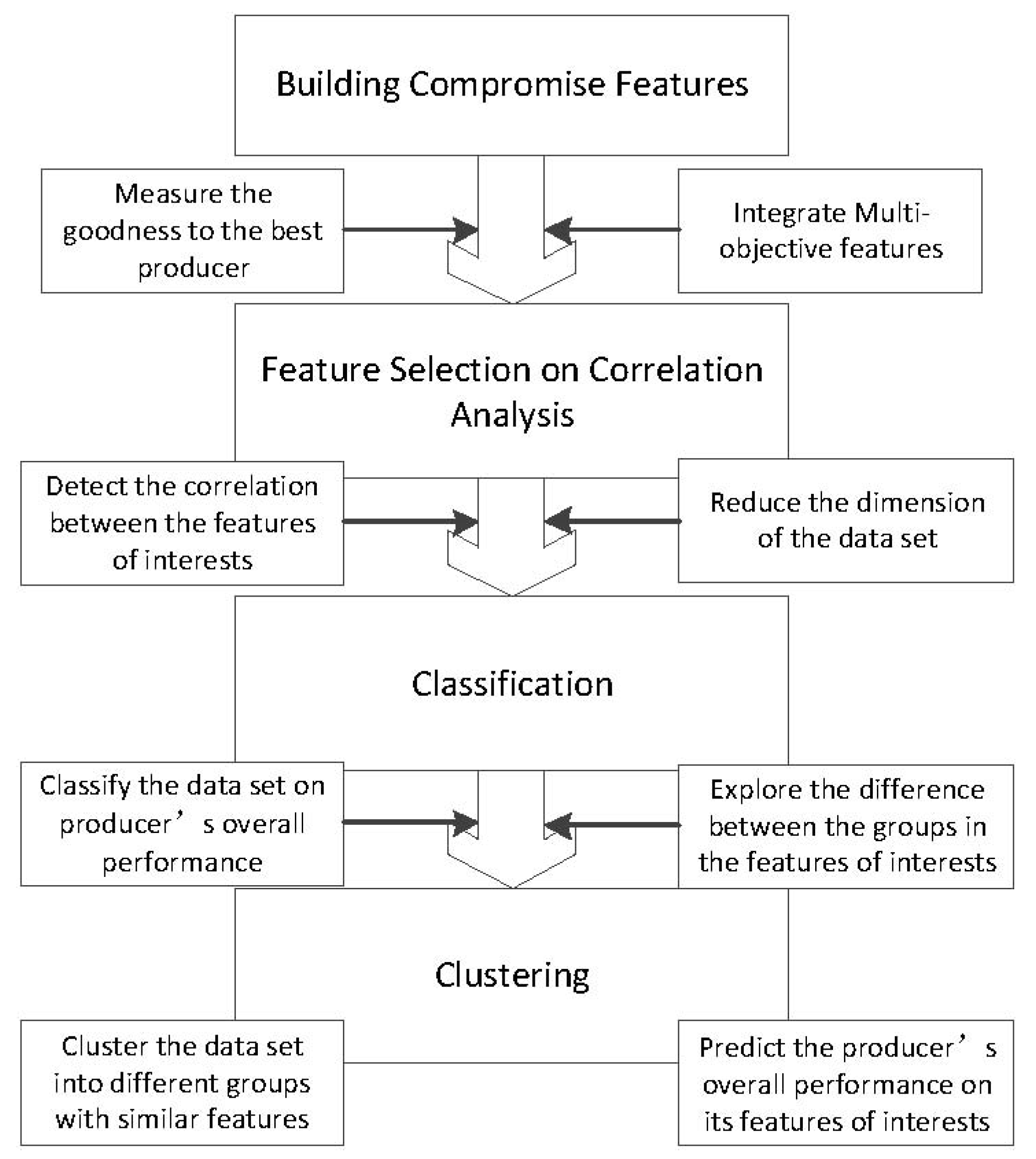
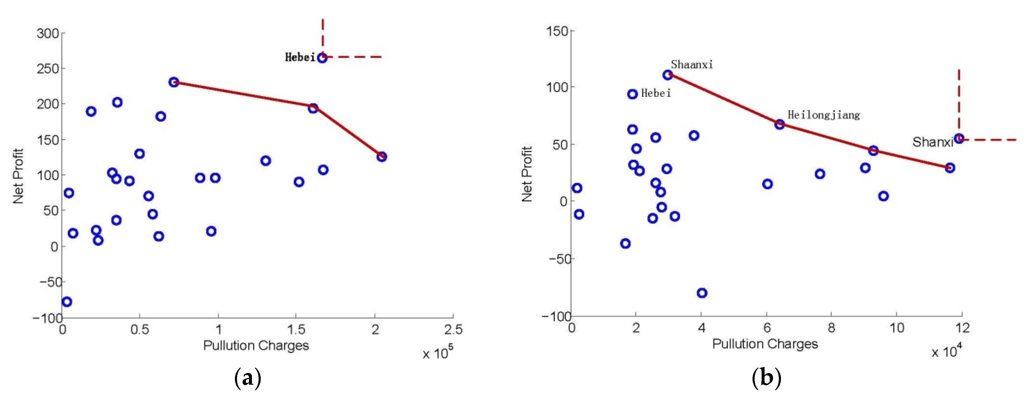
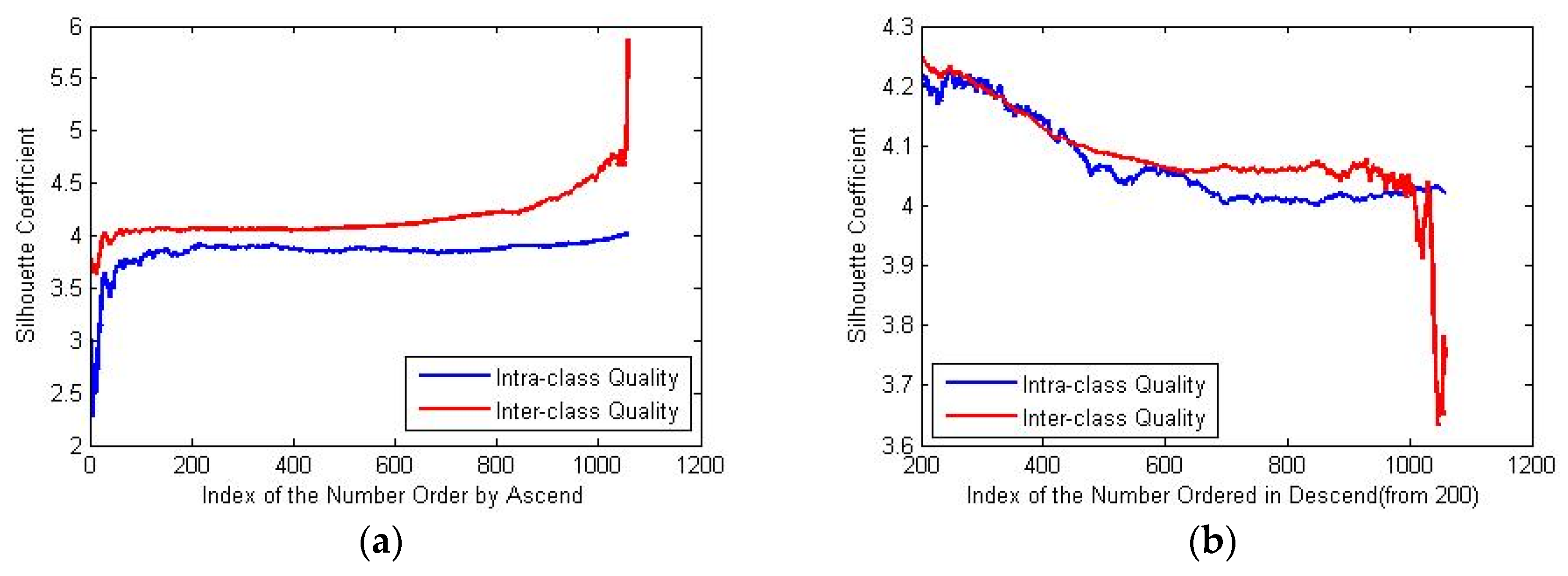
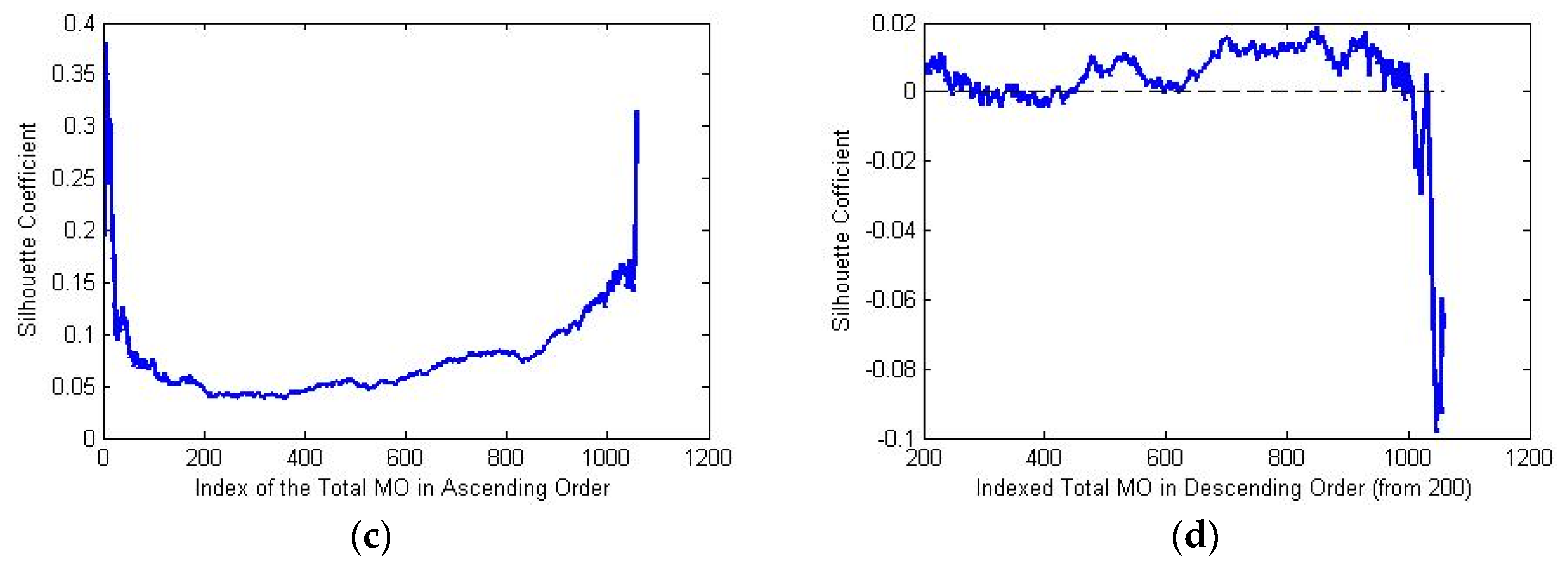
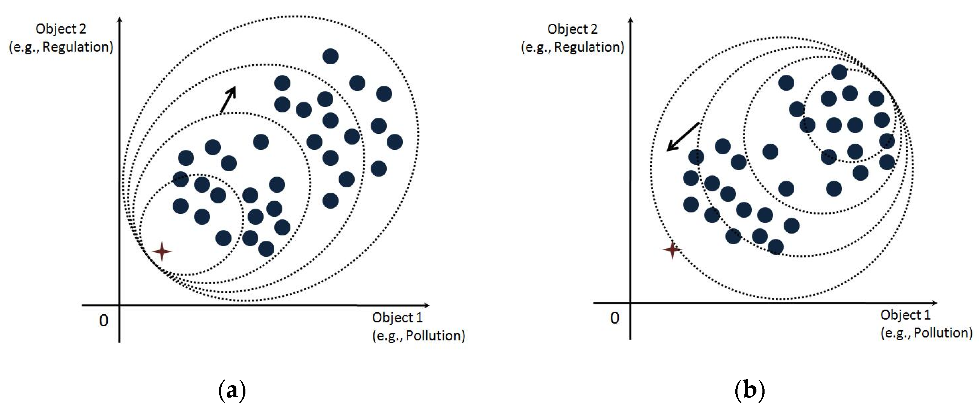
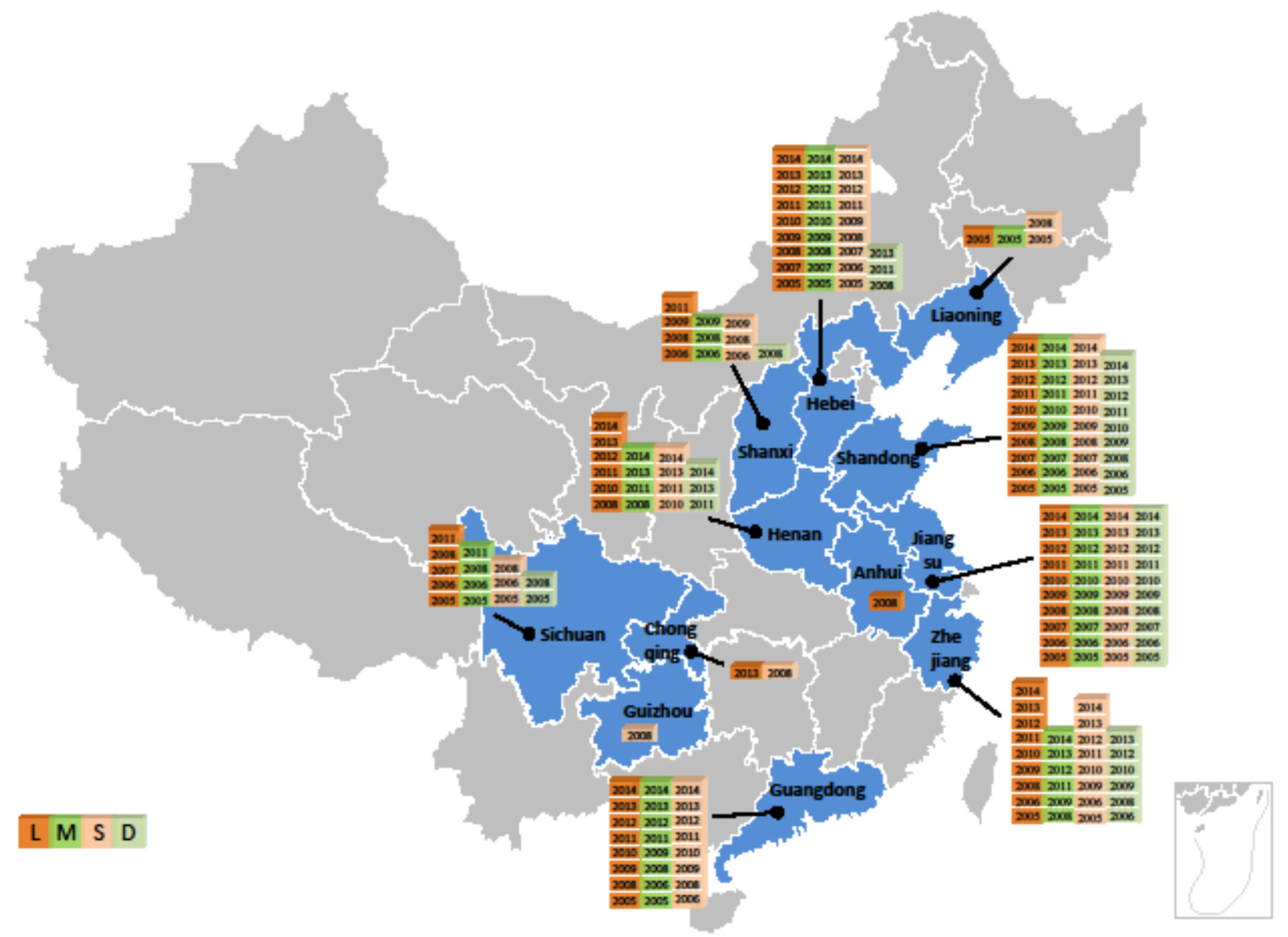
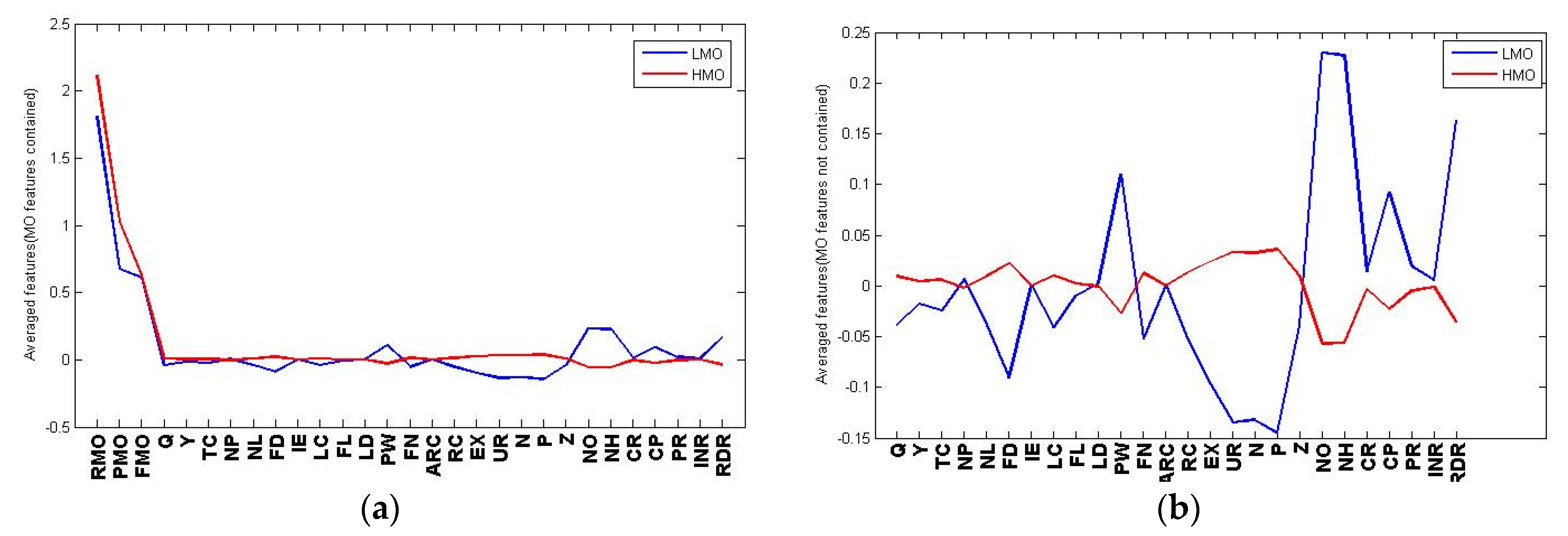
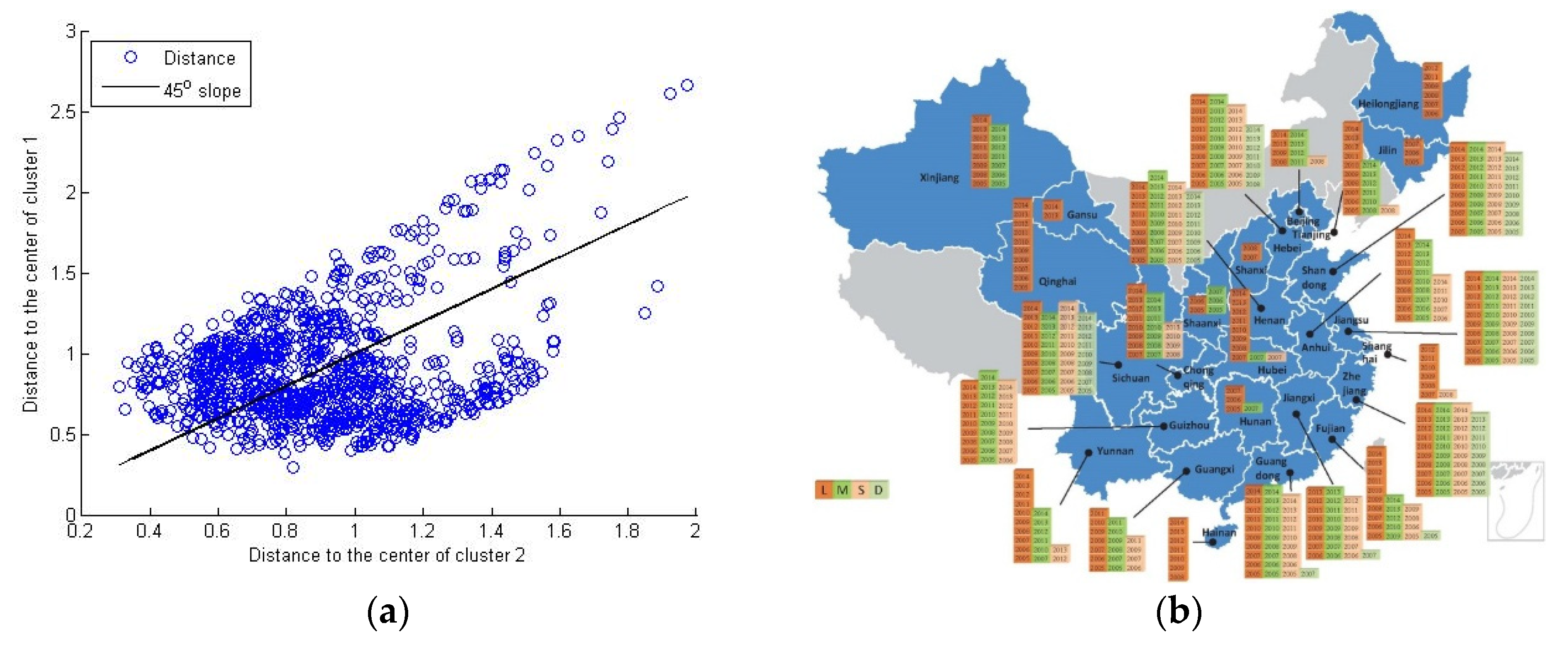
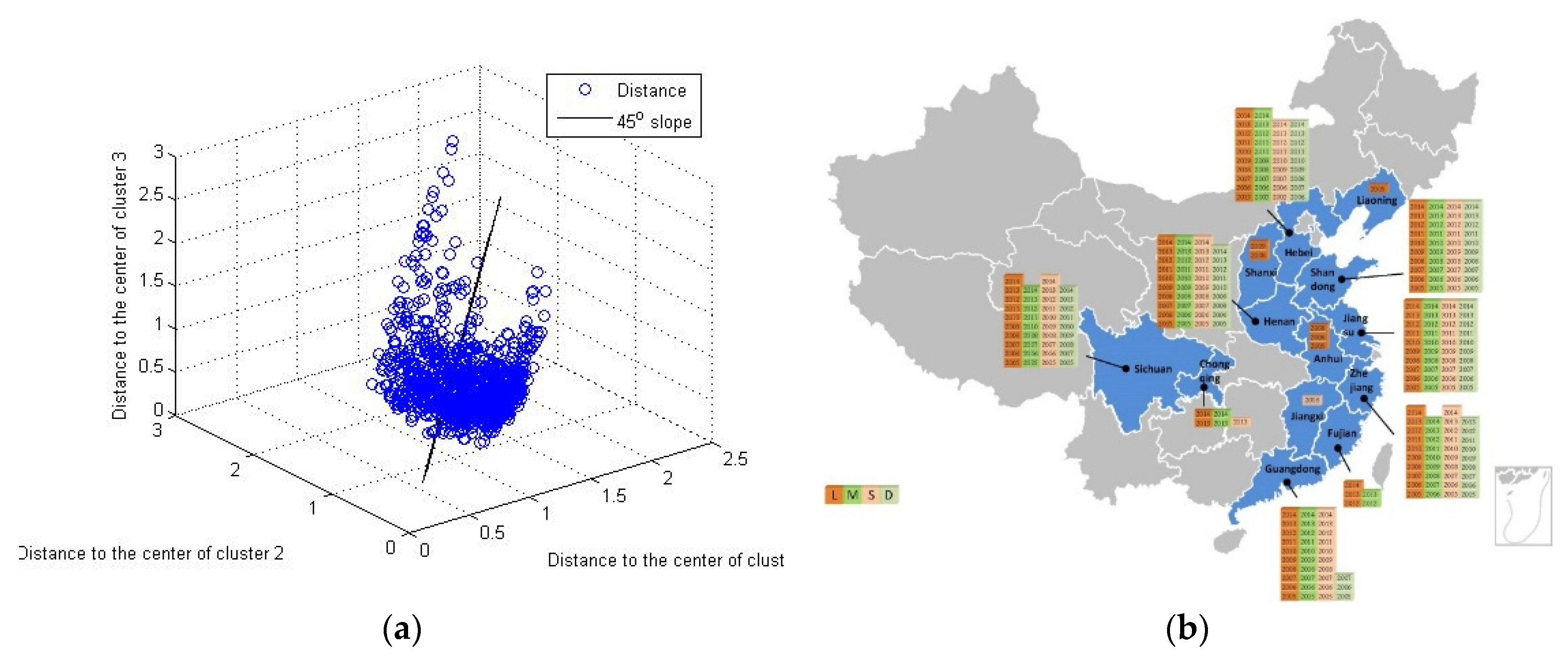
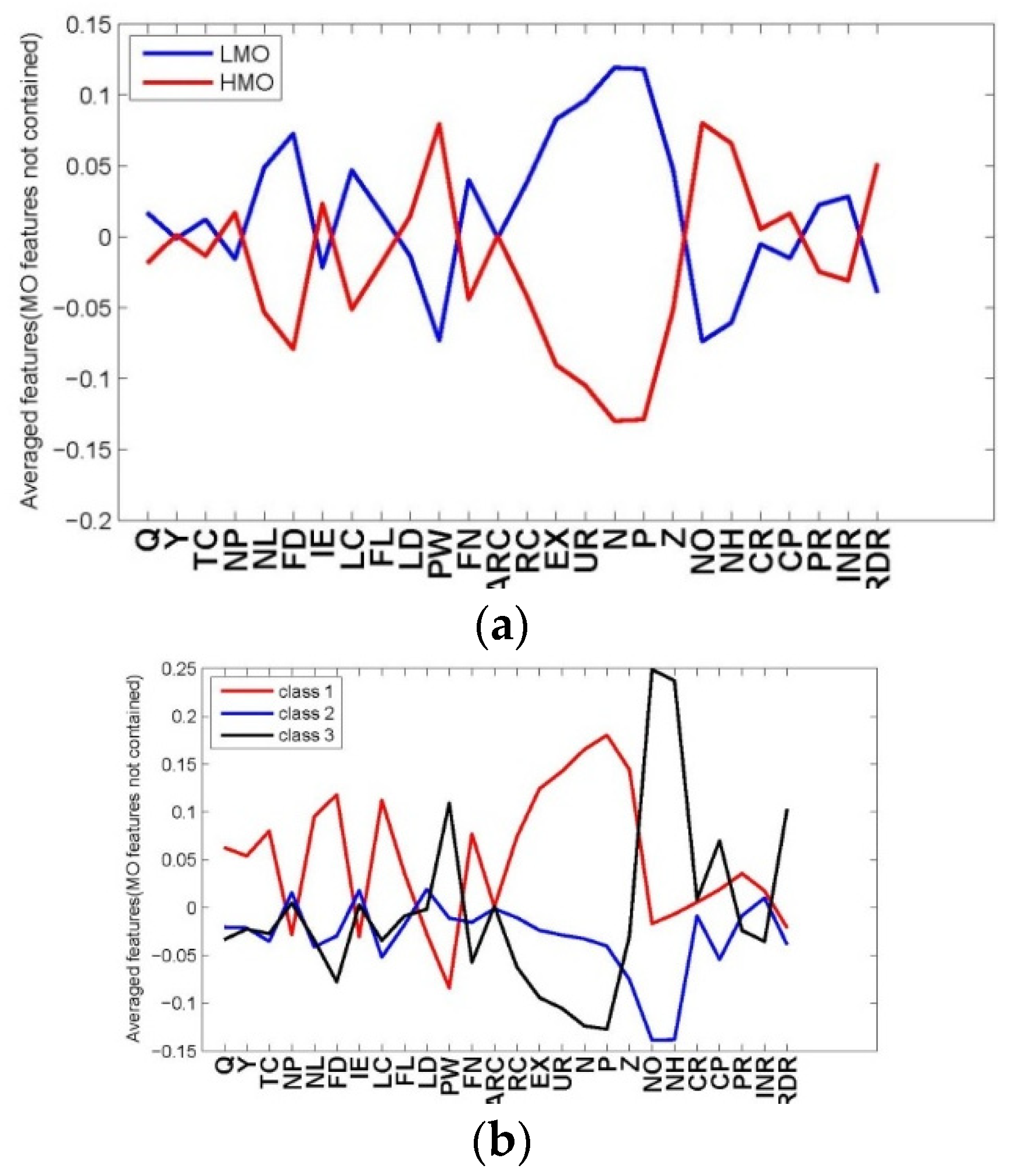


