Cropping System Diversification: Water Consumption against Crop Production

Abstract

This research reports on two pepper species cultivated in a pilot plot and protected under white shade nets during the 2014, 2015 and 2016 growing seasons. The goal of the study was to compare crop yield, water productivity, and economic productivity between sorghum and corn as extensive crops (ECs), and habanero peppers and bell peppers as intensive crops (ICs). The average values of crop yield, water productivity, and economic productivity were 4.8 Mg (Tons) ha⁻¹, 1.1 kg m⁻³, and 722.00 USD ha⁻¹ for sorghum; and 7.0 Mg ha⁻¹, 1.2 kg m⁻³, and 1390.00 USD ha⁻¹ for corn. Average values of 45.0 Mg ha⁻¹, 7.3 kg m⁻³, and 85,900.00 USD ha⁻¹; and 72.5 Mg ha⁻¹, 10.4 kg m⁻³, and 66,390.00 USD ha⁻¹ were obtained for habanero peppers and bell peppers, respectively—both were cultivated during 2014, 2015 and 2016. According to the climate conditions of this region, crop water requirements for pepper crops are 41.66% higher than for grain crops; nevertheless, the on-farm water application efficiencies are 92% and 58% respectively. Consequently, 11.97% more water is used for ICs than for ECs. The economic profitability for farmers was 72 times higher for intensive crops than for extensive crops.

1. Introduction

The green revolution brought with it mass production of staple cereals (wheat, rice, and corn) to solve the problem of feeding a growing population [1,2]. Worldwide, countries have devoted natural resources to cropping those grains, at times without proper planning to avoid indiscriminate losses of biodiversity [3,4,5]. Despite the profit gained from agricultural development in the last 65 years, problems such as a lack of equity, stability, and sustainability still remain major concerns for Latin American farmers. The advance of scientific knowledge focused on agricultural purposes (crop genetics, water-use efficiency, fertilizers, technological devices, intelligent algorithms, and so forth), as well as prices becoming more affordable to consumers, are without doubt intrinsic benefits of advances made during this time. However, land-use change, soil degradation, soil salinity, chemical pollution, groundwater depletion, and climate change emerge as the consequences of irrational cultivation [6,7,8,9,10,11].

While agriculture can improve the health, economics, and energetic aspects of society, it may also result in critical consequences for the environment, either through emissions of greenhouse gas or reduction in the quantity and quality of water and soil [12,13,14,15]. According to several studies [16,17,18], higher rates of damage to the environment tend to occur in regions with low per capita income. Such negative impacts are, in part, attributable to agriculture because of its use by governments as an economical mechanism to reduce rural poverty, mainly in developing countries [19,20]. Land-use change from non-agricultural land to agricultural land has several effects, such as a destabilized soil structure which modifies the regimes of stream and hortonian flow in the watersheds and increases soil erosion [13]. In terms of groundwater extraction, irrigated agriculture is the principal user of this water source, inducing an excessive exploitation of the aquifers and degrading groundwater-dependent ecosystems in the process [12]. Along these lines, several authors (e.g., Wang and Qiu [21]) have reported that agriculture is responsible for more than 70% of deforestation. Framework and index approaches have been developed for assessing environmental sustainability in agriculture [14,15,22], in an effort to implement policies to reduce agricultural pollution.

Mexico, as member of the United Nations (UN), signed an agenda in 2015 to address the end of poverty, pursuit of equity, and protection of the planet [23]. Among the 17 Sustainable Development Goals to be achieved by 2030 [24], Goal 1 (end poverty in all its forms everywhere), Goal 2 (end hunger, achieve food security and improved nutrition, and promote sustainable agriculture), and Goal 15 (sustainably manage forests, strike down desertification, halt and reverse land degradation, and halt biodiversity loss) are of particular interest for this study. Undeniably, agriculture can contribute to decreasing poverty and hunger, however it is imperative to carry it out using sustainable practices in order to reduce the irrational use of natural resources inherent to this economic activity. Diversification of cropping systems is a suitable alternative for farmers to increase their incomes in developing countries; furthermore, it plays an important positive role for the environment. Monocultures are the implicit target of crop diversification, which is an upcoming strategy that aims to improve the diversity of agricultural landscapes [25]. Monoculture agriculture is highly commercialized and a dominant system being adopted by developing countries [26]; nevertheless, it is widely accepted that monocultures have a deleterious effect on ecological conditions, placing higher pressure on biodiversity while being vulnerable to declining yields of crops [27,28,29]. Crop diversification refers to the shift from the dominance of one or just a few crops to the cultivation of a larger number of species [27]. Crop diversification offers several advantages over monocultures, such as soil fertility benefits, less damage from pests, drought mitigation, increasing the overall yield, and improving water and nutrient-use efficiencies [26,30,31]. Likewise, diversification can be an effective strategy for food and nutrition security, employment generation and the diminuition of poverty, by impacting agricultural growth [32].

Around 22.0 Mha are farmed annually in Mexico, from which 15.6 Mha is rainfed land while irrigation is applied to 6.4 Mha. The Mexican Northeast Bajo Río Bravo Irrigation District (RBID), one of the most important in the country, has historically been covered by almost 200,000 ha of sorghum (Sorghum bicolor L. Moench) crop (93% of the sowing surface) in the spring–summer season. During the fall–winter season, 7000 ha is established with corn (Zea mays L.) crop. In the past 25 years, the severity of droughts has increased in the Río Bravo watershed (a basin shared between the USA and Mexico), affecting agricultural production and livestock survival, with strong social and economic consequences for the region. These issues result in insufficient water to satisfy crop water requirements; as a consequence, alternatives have emerged to attempt to mitigate the phenomenon. Examples include the improvement of water-use efficiency, as well as productive reconversion privileging intensive crops over extensive ones.

This research reports on two pepper species cultivated in a pilot plot, protected under white shade nets, during 2014, 2015 and 2016. The goal of the study was to analyze the crop yield, water productivity, and economic productivity of sorghum and corn as extensive crops (ECs), compared with habanero peppers (Capsicum annum L.) and bell peppers (Capsicum chinense Jacq.) as intensive crops (ICs), in order to evidence differences between the cropping systems regarding water sustainability in terms of efficiency and productivity. The performance indicators of sorghum and corn crops were taken from agricultural statistics provided by the Secretariat of Agriculture, Livestock, Rural Development, Fisheries and Food (SAGARPA) and the National Water Commission of Mexico (CONAGUA). For pepper crops, a detailed study to compute the gross irrigation depth was completed, which included daily estimations of crop water requirements using the Food and Agriculture Organization (FAO) of the United Nations method, and drip irrigation scheduling through CropWat [33].

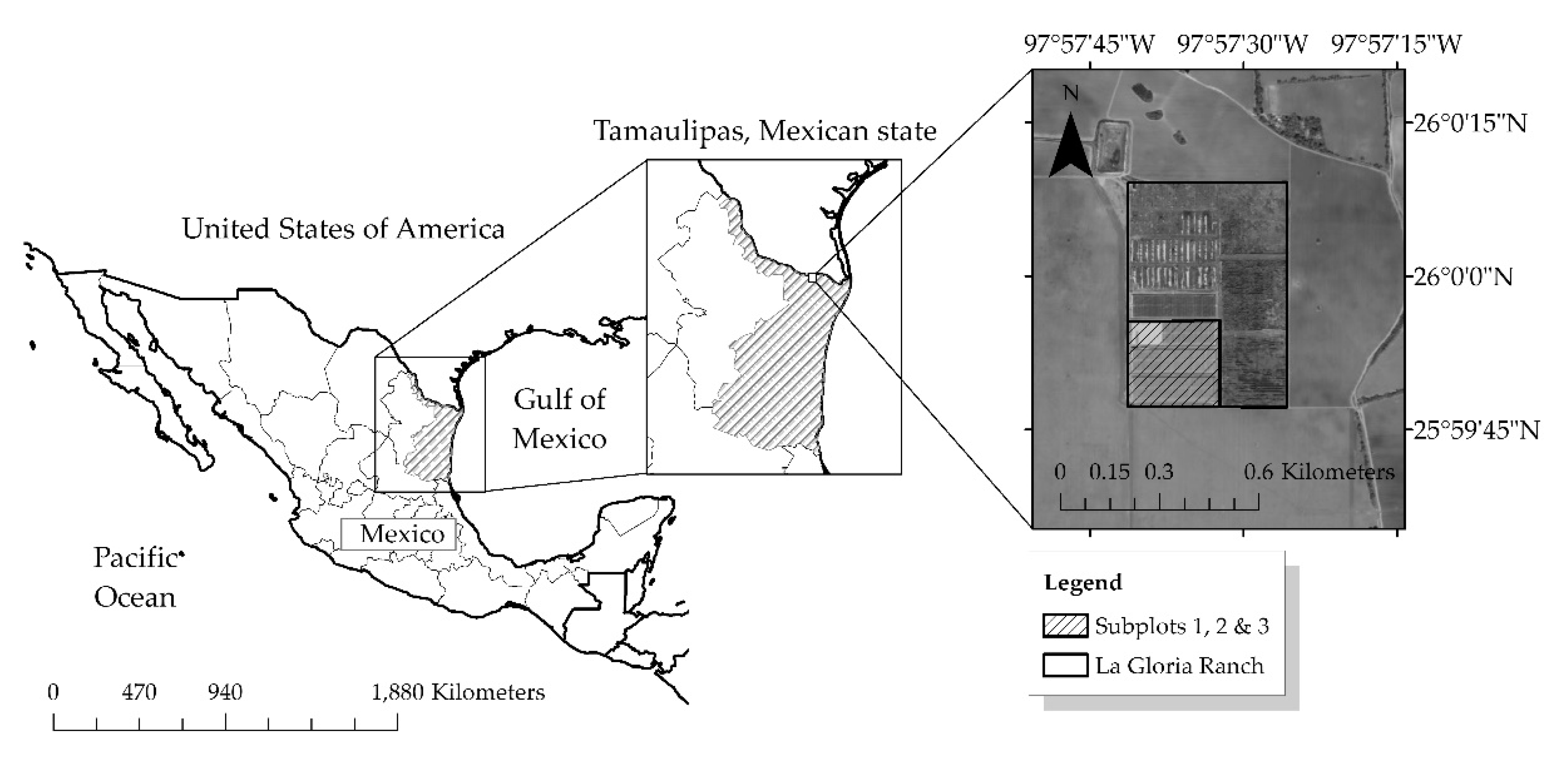
2. Materials and Methods

The experimental work was conducted during the 2014, 2015, and 2016 growing seasons at a commercial farm (La Gloria Ranch) (Figure 1) located in the RBID, 35 km east of the city of Reynosa, Mexico (25°59′54′′ N latitude; 97°57′40′′ W longitude; altitude 20 m above sea level). The soil is clay loam (average texture of 40.7% sand, 35.1% clay, and 24.2% silt) with 2.0% organic matter content, a field capacity of 0.40 m³ m⁻³, and a permanent wilting point of 0.22 m³ m⁻³. Such characteristics were obtained from 18 samples uniformly distributed along an experimental plot of 4.5 ha, established within the previously described commercial farm to depths of 0.30 m and 0.60 m (

Table 1. Soil properties following the Mexican norm NOM-021-RECNAT-2000.

Subplot	Sample	Depth	Granulometry			Texture	OMC	Soil Hydraulic Properties
		(cm)	Sand	Clay	Silt		(%)	Saturation	FC	PWP
			(%)	(%)	(%)			(%)	(m3 m−3)	(m3 m−3)
1	1	00–30	42.60	32.68	24.72	Clay Loam	1.8	51.25	0.38	0.21
		30–60	47.32	34.45	20.00	Sandy Clay Loam	1.9	53.03	0.40	0.20
	2	00–30	42.70	35.28	22.02	Clay Loam	1.8	52.24	0.37	0.22
		30–60	45.16	36.23	18.61	Sandy Clay	2.2	54.12	0.41	0.23
	3	00–30	41.15	34.16	24.69	Clay Loam	1.9	51.36	0.39	0.21
		30–60	44.19	34.53	21.28	Clay Loam	2.1	52.36	0.38	0.21
2	1	00–30	42.60	32.68	24.72	Clay Loam	2.2	51.25	0.38	0.21
		30–60	45.19	32.68	22.13	Sandy Clay Loam	1.9	52.24	0.38	0.20
	2	00–30	41.00	35.12	23.88	Clay Loam	2.1	52.94	0.40	0.23
		30–60	43.00	34.28	22.72	Clay Loam	2.0	52.66	0.39	0.22
	3	00–30	39.67	33.20	27.13	Clay Loam	1.9	52.73	0.39	0.22
		30–60	44.19	34.11	21.70	Clay Loam	2.1	52.55	0.39	0.21
3	1	00–30	38.96	32.68	28.36	Clay Loam	2.3	53.73	0.41	0.22
		30–60	31.32	47.04	21.64	Clay	2.1	55.10	0.46	0.28
	2	00–30	35.15	33.19	31.66	Clay Loam	1.8	53.00	0.39	0.22
		30–60	34.19	35.11	30.70	Clay Loam	2.0	53.44	0.41	0.23
	3	00–30	38.13	36.19	25.68	Clay Loam	1.9	53.32	0.40	0.23
		30–60	36.15	38.23	25.62	Clay Loam	1.9	53.77	0.42	0.24

OMC is the organic matter content; FC is the field capacity; PWP is the permanent wilting point.

). The texture and hydraulic parameters were performed following the Mexican norm NOM-021-RECNAT-2000, which establishes the methodology to classify agricultural soils [34]. The climate is semiarid with minimum and maximum mean monthly temperatures of 10.5 °C (December) and 34.6 °C (August), respectively. The average annual precipitation is approximately 697.0 mm, of which 40% occurs between September and October. Regarding evaporation, the mean yearly value is around 1750.0 mm—2.5 times higher than the rainfall rate.

The experimental plot was divided into three subplots (60 × 250 m) under the same agronomic conditions (e.g., fertilization depending on the requirements of each type of pepper). All subplots were netted to protect crops from environmental hazards and pests. Two experimental plots were sown with bell peppers, while the other one was sown with habanero peppers. The distance between rows was 0.80 m, and the average seedling density was approximately 45,000 plants ha⁻¹. Both pepper crops were suggested by the National Research Institute for Forestry, Agriculture, and Livestock of Mexico (INIFAP) as cultivars suited for irrigated land in that region of Mexico. Automated weather stations (Vantage Pro2 Davis Instruments) located inside every subplot were used to measure daily rainfall, daily average wind speed at 2 m above the ground surface, daily average relative humidity, daily minimum and maximum air temperatures, and daily total solar radiation. These data were used to estimate reference evapotranspiration (ET₀) by the United Nations Food and Agriculture Organization (FAO) Penman–Monteith method [35].

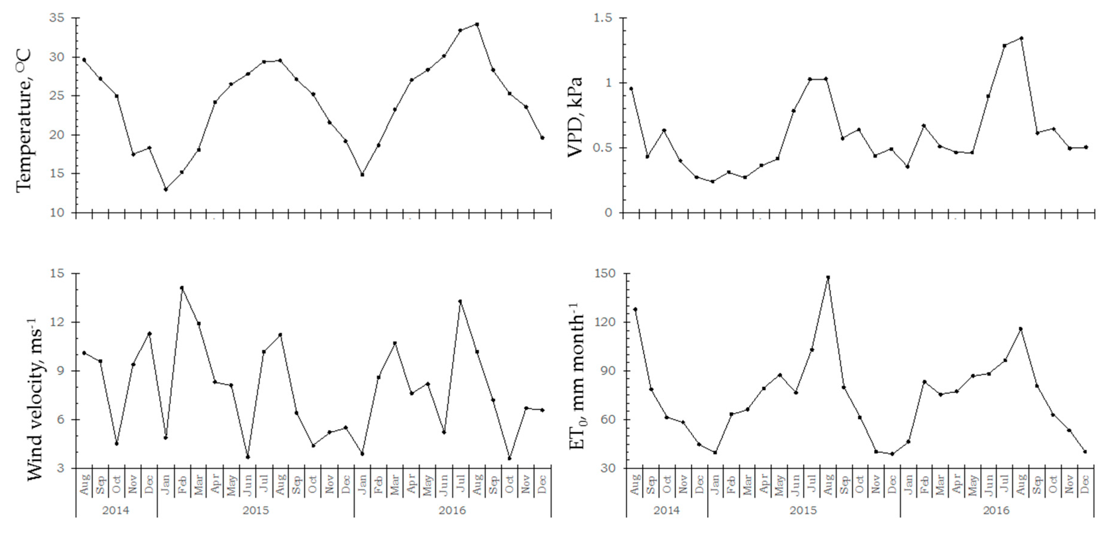
2.1. Net Corn Crop Water Requirements (CWR) and Irrigation Scheduling

A drip irrigation system was installed to irrigate the 1.5 ha subplots during all three spring–summer seasons. Net crop (habanero pepper and bell pepper) water requirements were computed as follows:

$$\mathrm{CWR}={\mathrm{ET}}_{\mathrm{c}}-\mathrm{PEF}$$

(1)

where CWR (mm) is the water required by the crop to compensate for the loss of water through evapotranspiration; ET_c (mm) is the crop evapotranspiration (Equation (2)); and PEF (mm) is the effective precipitation. Equation (1) was applied on a weekly basis. The values for ET_c and PEF were estimated as follows:

$${\mathrm{ET}}_{\mathrm{c}}={\displaystyle \sum }_{\mathrm{i}=\mathrm{t}}^{\mathrm{T}}{\mathrm{K}}_{\mathrm{ci}}{\mathrm{ET}}_{0\mathrm{i}}$$

(2)

where ET_0i (mm) is the reference evapotranspiration for day i; K_ci is the crop coefficient for day i; t is the first day of the considered period; and T is the last day of the considered period. To estimate the crop coefficients, the FAO methodology was followed. The FAO proposed defining four phenological stages (initial, development, midseason, and late stages), estimating three Kc values (initial season, Kc_ini; midseason, Kc_mid; and late season, Kc_end), and connecting straight line segments through each of the four growth stages [35]. Horizontal lines are drawn through Kc in the initial and midseason stages, whereas diagonal lines are drawn from Kc_ini to Kc_mid during the course of the development stage and from Kc_mid to Kc_end during the course of the late-season stage. The Kc length of the stages recommended by Allen et al. [35] were used in this paper to estimate Kc. The Kc values for the initial season, midseason, and late season were Kc_ini = 0.60, Kc_mid = 1.05, and Kc_end = 0.90, respectively, with lengths of 30 d for the initial stage, 40 d for the development stage, 110 d for the midseason stage, and 30 d for the late stage.

$$\begin{gathered} \mathrm{PEF}=0.75\mathrm{P}\mathrm{if}\mathrm{P}>0.2{\mathrm{ET}}_{0\mathrm{s}} \\ \mathrm{PEF}=0.00\mathrm{if}\mathrm{P}\le 0.2{\mathrm{ET}}_{0\mathrm{s}} \end{gathered}$$

(3)

where P (mm) is the precipitation for the considered period, and ET_0s (mm) is the reference evapotranspiration for the considered period. The irrigation gross depth (IGD; mm) was calculated as follows:

$$\mathrm{IGD}=\frac{\mathrm{CRW}}{{\mathrm{E}}_{\mathrm{a}}}$$

(4)

where E_a is the application efficiency. For all seasons, irrigation water was applied by a drip irrigation system with 0.20 cm spacing between the emitters. Model 6000 Aqua-traxx tape, manufactured by The Toro Company (El Cajon, CA, USA), was used in the experiment. The system operated at 55 kPa of hydraulic pressure. For pressures between 55 kPa and 70 kPa, when driplines were used, six preliminary experimental tests were performed to determine the coefficient of uniformity (CU) and the low-quarter distribution uniformity (DU) [36,37] of the water application under two different emitter discharges (0.75 L/h, and 0.85 L/h), following the criteria outlined by Merriam and Keller [38]. CU values of 93%, 92%, 96%, 94%, 96% and 93%, and DU values of 89%, 90%, 96%, 92%, 90%, and 90%, were obtained for the emitter discharges. Taking into account the CU and DU indicators, an average application efficiency of 92% was claimed by the tape producer. Regarding the E_a used for corn and sorghum, CONAGUA [39] carried out a study to modernize the RBDI; among the main findings, an average application efficiency of 58% was established. This value was taken into account to quantify the irrigation gross depth for both of the extensive crops that were analyzed.

2.2. Statistical Analysis

Levene’s test was used to assess the equality of variances (homoscedasticity) between average values in ICs and ECs in three performance indicators (grain yield, water productivity and economic productivity). Once the homoscedasticity was evaluated, the Student’s t-test was performed; the t-test compares two means and evaluates how significant the differences are. The null hypothesis assumed that the values between ICs and ECs are similar; otherwise, the alternative hypothesis establishes that those values are different. All statistical analyses were performed in SPSS Statistics 17.0^® [40,41,42].

3. Results and Discussion

The meteorological conditions inside of the cover subplots for the 2014, 2015, and 2016 crop seasons are presented in Figure 2, as the averages of the data reported for the three weather stations used in the study. Air temperature averages were 23.5 °C, 23.1 °C, and 25.6 °C for 2014, 2015, and 2016, respectively. The minimum and maximum air temperature values were 17.5 °C and 29.6 °C, respectively, for 2014; 13.0 °C and 29.5 °C, respectively, for 2015; and 14.9 °C and 34.2 °C, respectively, for 2016. The vapor-pressure deficit (VPD) ranged from 0.27–0.95 kPa for 2014, from 0.24–1.03 kPa for 2015, and from 0.36–1.34 kPa for 2016. The averages of these values were 0.54 kPa, 0.55 kPa and 0.69 kPa, respectively. The wind speed was higher for 2014 than 2015 and 2016. The mean monthly values were 9.0 m s⁻¹, 7.8 m s⁻¹ and 7.7 m s⁻¹, although maximum gusts of 13.8 m s⁻¹ (in 2014), 16.8 m s⁻¹ (in 2015), and 13.8 m s⁻¹ (in 2016) were reached. In accordance with these differences in meteorological conditions, there also were some differences between the corresponding estimates of ET₀ (Figure 2). The ET₀ ranged from 44.6–127.9 mm month⁻¹ for 2014, from 38.8–147.6 mm month⁻¹ for 2015, and from 40.1–115.7 mm month⁻¹ for 2016. The average ET₀ values were 74.1 mm month⁻¹ for 2014, 73.6 mm month⁻¹ for 2015, and 75.5 mm month⁻¹ for 2016. The main difference in ET₀ among seasons was observed during July and August, when ET₀ rates were much higher. This difference was mainly attributable to the higher VPD values observed during this time period (Figure 2). The increase in ET₀ and VPD observed for the summer period for each year was caused by higher temperatures recorded during this period. Precipitation in summer is low at the study area, leading to higher temperatures and a slight reduction of the humidity of the air.

The values of the net crop water requirements (CWR, Equation (1)), irrigation gross depth (IGD, Equation (4)), and effective precipitation (PEF, Equation (3)), estimated for each year of experimentation, are presented in

Table 2. Crop water requirements (CWR), irrigation gross depth (IGD), and effective precipitation (PEF) values for the 2014, 2015, and 2016 crop seasons in the RBID Mexican region.

Year	Season	CWR (mm)				IGD (mm)				PEF (mm)
		Corn	Sorghum	Habanero	Bell	Corn	Sorghum	Habanero	Bell
				Pepper *	Pepper *			Pepper	Pepper
2014	FW	409.38	401.75	564.12	639.33	705.83	692.67	613.17	694.92	0
2015	SS	459.02	458.25	—	—	791.41	790.09	—	—	0
	FW	381.33	410.25	574.52	644.51	657.47	707.33	624.48	700.55	318.16
2016	SS	474.96	468.93	—	—	818.9	808.5	—	—	91.25
	FW	399.41	411.76	570.22	640.93	688.64	709.93	619.8	696.66	213.16

FW is Fall-Winter crop season; SS is Spring-Summer crop season; * Differences between CWRs for pepper crops are associated with sown date.

. The CWRs for extensive crops are less than for intensive crops (the average CWR is around 41.66% higher for ICs than ECs). This difference is attributed to the phenological properties of ECs and ICs [35]. However, these conditions change when the application efficiency factor is included to consider water losses during irrigation events; the average value of the IGD was 11.97% higher for ECs than ICs because irrigation methods used to irrigate corn and sorghum were 34% less efficient than those used to irrigate habanero peppers and bell peppers in the experimental subplots [39]. This is consistent with the findings reported by Bautista-Capetillo et al. [43]. In accordance with the noted results, rational agricultural water use requires the execution of technical and economical strategies regarding irrigation methods, in order to increase on-farm efficiency without compromising crop production.

The production of corn and sorghum represents 14.47% and 2.24%, respectively, of the agricultural growth domestic product (GDP), which makes them two of the key crops for economic development in the region. In Mexico, corn production accounts for over two-thirds of the gross value of agricultural production [44,45,46]. Crop yield, water productivity, and the economic productivity of extensive grains were obtained from agricultural and food information provided by the Mexican Government [47] for the period 2014–2016. The average yearly values as the result of the spring-summer and fall-winter crop seasons were 4.8 Mg ha⁻¹, 1.1 kg m⁻³, and 722.00 USD ha⁻¹ for sorghum; and 7.0 Mg ha⁻¹, 1.2 kg m⁻³, and 1390.00 USD ha⁻¹ for corn (

Table 3. Performance indicators for the 2014, 2015, and 2016 crop seasons in the RBID Mexican 234 region for extensive crops (ECs).

Year	Crop Yield		Water Productivity		Economic Productivity
	(Mg ha−1)		(kg m−3)		(US ha−1)
	Sorghum	Corn	Sorghum	Corn	Sorghum	Corn
2014	5.15	7.28	1.14	1.25	731.77	1425.28
2015	4.71	6.99	1.10	1.20	741.45	1370.81
2016	4.65	7.00	1.10	1.20	693.04	1373.75

).

Table 4. Performance indicators for the 2014, 2015, and 2016 crop seasons in the RBID Mexican region for intensive crops (ICs).

Year	Grain Yield		Water Productivity		Economic Productivity
	(Mg ha−1)		(kg m−3)		(US ha−1)
	Habanero	Bell	Habanero	Bell	Habanero	Bell
	Pepper	Pepper	Pepper	Pepper	Pepper	Pepper
2014	41.50	73.60	6.77	10.59	82,625.00	62,560.00
2015	45.80	71.00	7.33	10.13	91,600.00	67,450.00
2016	47.70	72.80	7.70	10.45	83,475.00	69,160.00

shows the same performance indicators, but for habanero peppers and bell peppers, cultivated during the 2014, 2015, and 2016 crop seasons. The average values were 45.0 Mg ha⁻¹, 7.3 kg m⁻³, and 85,900.00 USD ha⁻¹; and 72.5 Mg ha⁻¹, 10.4 kg m⁻³, and 66,390.00 USD ha⁻¹ for habanero peppers and bell peppers, respectively.

Table 5. Results from the Levene’s test for equality of variances.

Performance Indicators	Levene’s Test for Equality of Variances
	F	Significance
Grain Yield	0.215	0.667
Water Productivity	10.774	0.030
Economic Productivity	4.584	0.100

shows the results from the Levene’s test, which indicate that the IC and EC values have equal variances for the grain yield and economic productivity indicators, and different variance for water productivity with 10% significance. Once the homoscedasticity was evaluated, the t-test was performed (

Table 6. Results from the t-test for equality of means.

Performance Indicators	t-Test for Equality of Means
						95% Confidence Interval of Difference
	t	Df *	Sig ** (2-Tailed)	Mean Difference	Std. Error Difference	Lower	Upper
Grain Yield	42.676	4.00	<0.001	51.975	1.21879	48.53359	55.35641
Water Productivity	61.246	2.06	<0.001	7.663	0.12512	7.13964	8.18636
Economic Productivity	37.486	4.00	<0.001	75,088.980	2003.14	69,527.37	80,650.58

* df is degrees of freedom, ** Sig. is significance.

). The results indicate that there are important differences among the means of the three performance indicators with a significance of p < 0.001. To perform the t-test in the water productivity indicator (equal variances not assumed), a correction was done by SPSS.

The performance indicators (grain yield, water productivity, and economic productivity) were significantly (p < 0.001) different between ICs and ECs; approximately 10 times for the crop yield, 9 times for water productivity, and 72 times for economic productivity. It should be noted that pepper yields exceeded the average yield for the climatic conditions of the Tamaulipas region (30.0 Mg ha⁻¹ and 60.0 Mg ha⁻¹ for habanero peppers and bell peppers, respectively) [48,49]. This yield increase is in agreement with results obtained in previous research [43,50,51] where variables that condition the crop growth to satisfy crop water requirements were rigorously monitored. Regarding the productivity extents (Table 3), the quantity of water per unit of produced crop pays better dividends for ICs than ECs, an aspect that by itself stands out as a better use of water resources; however, the economic competitiveness that pepper crops represent in the commercial market compared with grain crops should not be ignored. On the other hand, it is noted that on-farm water application plays a significant role in the sustainability of this natural resource [52,53,54]. Areas cultivated with grain crops that need a certain volume of water have to apply around 42% more water to be assured of adequate development along all crop phenological stages, while for pepper crops only 8% of the water used can be considered as a loss (Table 2). These variances in application efficiency should influence the discussion regarding whether water resources are really being used rationally. Of course, both cropping systems are essential in a developing country such as Mexico, but there are substantial differences between the systems. In particular, consideration should be given to the relationship between the vast expanses of land required to cultivate corn or sorghum in order to generate economic profitability for farmers, with the consequent financial incentive to establish hydraulic and agronomic schemes that contribute to more efficient use of water. In light of these results, agricultural water resource management implies the use of stricter policies to be put into practice by users; nevertheless, their implementation requires the economical, technical, and regulatory support of government.

4. Conclusions

Increases in water requests among various water users demands effective strategies for rationing this resource without compromising the production of commodities. In the Mexican agricultural sector, application efficiency still prevails as one factor of great importance, especially in extensive cropping systems where economic benefits for producers hinder the implementation of infrastructure to irrigate more efficiently. This work reports on the comparison between water consumption and crop production for extensive and intensive agriculture in the Bajo Río Bravo Irrigation District in the northeast of Mexico. According to the climate conditions of this region, crop water requirements for pepper crops (an intensive cropping system) are 41.66% higher than for grain crops (an extensive cropping system); nevertheless, the on-farm water application efficiencies are 92% for pepper crops and 58% for grain crops. Consequently, 11.97% more water is used for corn and sorghum crops than for habanero pepper and bell pepper crops. Despite both cropping systems being indispensable for economic development in Mexico, the economic profitability for farmers was 72 times higher for intensive crops than for extensive crops; an important difference between the average values for three performance indicators was found in accordance with the statistical tests. Because of this, our research provides new information about cropping systems, as well as agricultural performance indicators to contribute to the sustainability of water use.

References

1. Conway, G.R.; Barbier, E.B. After the Green Revolution: Sustainable Agriculture for Development, 1st ed.; Easthscan Publications Ltd.: London, UK, 1990; ISBN 1-85383-035-6. [Google Scholar]
2. Martin-Guay, M.-O.; Paquette, A.; Dupras, J.; Rivest, D. The new Green Revolution: Sustainable intensification of agriculture by intercropping. Sci. Total Environ. 2018, 615, 767–772. [Google Scholar] [CrossRef] [PubMed]
3. Foley, J.A.; DeFries, R.; Asner, G.P.; Barford, C.; Bonan, G.; Carpenter, S.R.; Chapin, F.S.; Coe, M.T.; Daily, G.C.; Gibbs, H.K.; et al. Global Consequences of Land Use. Science 2005, 309, 570–574. [Google Scholar] [CrossRef] [PubMed] [Green Version]
4. Foley, J.A.; Ramankutty, N.; Brauman, K.A.; Cassidy, E.S.; Gerber, J.S.; Johnston, M.; Mueller, N.D.; O’Connell, C.; Ray, D.K.; West, P.C.; et al. Solutions for a cultivated planet. Nature 2011, 478, 337–342. [Google Scholar] [CrossRef] [PubMed] [Green Version]
5. Tilman, D.; Cassman, K.G.; Matsons, P.A.; Naylor, R.; Polasky, S. Agricultural sustainability and intensive production practices. Nature 2002, 418, 671–677. [Google Scholar] [CrossRef] [PubMed] [Green Version]
6. Noya, I.; González-García, S.; Bacenetti, J.; Fiala, M.; Moreira, M.T. Environmental impacts of the cultivation-phase associated with agricultural crops for feed production. J. Clean. Prod. 2018, 172, 3721–3733. [Google Scholar] [CrossRef]
7. Chen, Y.-H.; Wen, X.-W.; Wang, B.; Nie, P.-Y. Agricultural pollution and regulation: How to subsidize agriculture? J. Clean. Prod. 2017, 164, 258–264. [Google Scholar] [CrossRef]
8. Evenson, R.E.; Gollin, D. Assessing the Impact of the Green Revolution, 1960 to 2000. Science 2003, 300, 758–762. [Google Scholar] [CrossRef] [PubMed]
9. Environmental Impacts of Farming. Available online: http://wwf.panda.org/our_work/food/agriculture/impacts/ (accessed on 18 May 2018).
10. Urso, J.H.; Gilberston, L.M. Atom Conversion Efficiency: A New Sustainability Metric Applied to Nitrogen and Phosphorus Use in Agriculture. ACS Sustain. Chem. Eng. 2018, 6, 4453–4463. [Google Scholar] [CrossRef]
11. Capa, D.; Pérez-Esteban, J.; Masaguer, A. Unsustainability of recommended fertilization rates for coffee monoculture due to high N2O emissions. Agron. Sustain. Dev. 2015, 35, 1551–1559. [Google Scholar] [CrossRef]
12. Tweed, S.; Celle-Jeanton, H.; Cabot, L.; Huneau, F.; De Montety, V.; Nicolau, N.; Travi, Y.; Babic, M.; Aquilina, L.; Vergnaud-Ayraud, V.; et al. Impact of irrigated agriculture on groundwater resources in a temperate humid region. Sci. Total Environ. 2018, 613–614, 1302–1316. [Google Scholar] [CrossRef] [PubMed]
13. Ouyang, W.; Wu, Y.; Hao, Z.; Zhang, Q.; Bu, Q.; Gao, X. Combined impacts of land use and soil property changes on soil erosion in a mollisol area under long-term agricultural development. Sci. Total Environ. 2018, 613–614, 798–809. [Google Scholar] [CrossRef] [PubMed]
14. Scharfy, D.; Boccali, N.; Stucki, M. Clean Clean Technologies in Agriculture—How to Prioritise Measures? Sustainability 2017, 9, 1303. [Google Scholar] [CrossRef]
15. Hale, I.L.; Wollheim, W.M.; Smith, R.G.; Asbjornsen, H.; Brito, A.F.; Broders, K.; Grandy, A.S.; Rowe, R. A Scale-Explicit Framework for Conceptualizing the Environmental Impacts of Agricultural Land Use Changes. Sustainability 2014, 6, 8432–8451. [Google Scholar] [CrossRef] [Green Version]
16. Kelly, T.J.; Gîthînji, M. Environmental Degradation and Poverty in Less Industrialized Nations. Front. Norte 1994, 6, 77–90. [Google Scholar]
17. Pretty, J.N.; Morison, J.I.L.; Hine, R.E. Reducing food poverty by increasing agricultural sustainability in developing countries. Agric. Ecosyst. Environ. 2003, 95, 217–234. [Google Scholar] [CrossRef]
18. Pretty, J.N.; Noble, A.D.; Bossio, D.; Dixon, J.; Hine, R.E.; Penning de Vries, F.W.T.; Morrison, J.I.L. Resource-Conserving Agriculture Increases Yields in Developing Countries. Environ. Sci. Technol. 2006, 40, 1114–1119. [Google Scholar] [CrossRef] [PubMed] [Green Version]
19. Cazzuffi, C.; Pereira-Lopez, M.; Soloaga, I. Local poverty reduction in Chile and Mexico: The role of food manufacturing growth. Food Policy 2017, 68, 160–185. [Google Scholar] [CrossRef]
20. Mellor, J.W.; Malik, S.J. The Impact of Growth in Small Commercial Farm Productivity on Rural Poverty Reduction. World Dev. 2017, 91, 1–10. [Google Scholar] [CrossRef]
21. Wang, H.; Qiu, F. Investigating the Impact of Agricultural Land Losses on Deforestation: Evidence from a Peri-urban Area in Canada. Ecol. Econ. 2017, 139, 9–18. [Google Scholar] [CrossRef]
22. Sabiha, N.-E.; Salim, R.; Rahman, S.; Rola-Rubzen, M.F. Measuring environmental sustainability in agriculture: A composite environmental impact index approach. J. Environ. Manag. 2016, 166, 84–93. [Google Scholar] [CrossRef] [PubMed]
23. Imaz, M.; Sheinbaum, C. Science and technology in the framework of the sustainable development goals. World J. Sci. Technol. Sustain. Dev. 2017, 14, 2–17. [Google Scholar] [CrossRef]
24. United Nations (UN); 17 Sustainable Development Goals (SDGs). 2030 Agenda for Sustainable Development; UN Publishing: New York, NY, USA, 2018. [Google Scholar]
25. Mahy, L.; Dupeux, B.E.T.I.; Van Huylenbroeck, G.; Buysse, J. Simulating farm level response to crop diversification policy. Land Use Policy 2015, 45, 36–42. [Google Scholar] [CrossRef]
26. Kasem, S.; Thapa, G.B. Crop diversification in Thailand: Status, determinants, and effects on income and use of inputs. Land Use Policy 2011, 28, 618–628. [Google Scholar] [CrossRef]
27. Monteleone, M.; Cammerino, A.R.B.; Libutti, A. Agricultural “greening” and cropland diversification trends: Potential contribution of agroenergy crops in Capitana (South Italy). Land Use Policy 2018, 70, 591–600. [Google Scholar] [CrossRef]
28. Yang, X.; Chen, Y.; Pacenka, S.; Gao, W.; Ma, L.; Wang, G.; Yan, P.; Sui, P.; Steenhuis, T. Effect of diversified crop rotations on groundwater levels and crop water productivity in the North China Plain. J. Hydrol. 2015, 522, 428–438. [Google Scholar] [CrossRef]
29. Yang, X.; Gao, W.; Zhang, M.; Chen, Y.; Sui, P. Reducing agricultural carbon footprint through diversified crop rotation systems in the North China Plain. J. Clean. Prod. 2014, 76, 131–139. [Google Scholar] [CrossRef]
30. Alam, M.J.; Humphreys, E.; Sarkar, M.A.R. Intensification and diversification increase land and water productivity and profitability of rice-based cropping systems on the High Ganges River Floodplain of Bangladesh. Field Crops Res. 2017, 209, 10–26. [Google Scholar] [CrossRef]
31. Andrade, J.F.; Poggio, S.L.; Ermácora, M.; Satorre, E.H. Land use intensification in the Rolling Pampa, Argentina: Diversifyingcrop sequences to increase yields and resource use. Eur. J. Agron. 2016, 82, 1–10. [Google Scholar] [CrossRef]
32. Birthal, P.S.; Joshi, P.K.; Roy, D.; Thorat, A. Diversification in Indian Agriculture toward High-Value Crops: The Role of Small Farmers. Can. J. Agric. Econ. 2013, 61, 61–91. [Google Scholar] [CrossRef]
33. Broumer, C.; Prins, K.; Heibloem, M. Irrigation Water Management: Irrigation Scheduling; Food and Agriculture Organization of the United Nations (FAO): Rome, Italy, 1989. [Google Scholar]
34. Secretaria de Medio Ambiente y Recursos Naturales (SEMARNAT). NORMA Oficial Mexicana NOM-021-RECNAT-2000; Government of Mexico: México City, México, 2002. [Google Scholar]
35. Allen, R.G.; Pereira, L.S.; Raes, D.; Smith, M. Crop Evapotranspiration: Guidelines for Computing Crop Water Requirements; Paper 56; Food and Agriculture Organization of the United Nations: Rome, Italy, 1998. [Google Scholar]
36. Christiansen, J.E. Irrigation by Sprinkling; California Agricultural Experiment Station Bulletin 670; Univeristy of California, Berkeley: Berkeley, CA, USA, 1942. [Google Scholar]
37. Burt, C.M.; Clemmens, A.J.; Strelkoff, T.S.; Solomon, K.H.; Bliesner, R.D. Irrigation Performance Measures, Efficiency and Uniformity. In Biological Systems Engineering: Papers and Publications; Available online: https://digitalcommons.unl.edu/cgi/viewcontent.cgi?article=1038&context=biosysengfacpub (accessed on 21 June 2018).
38. Merriam, J.L.; Keller, J. Farm Irrigation System Evaluation: A Guide for Management; Utah State University: Logan, UT, USA, 1978. [Google Scholar]
39. Comision Nacional del Agua (CONAGUA). Modernización y Tecnificación del Distrito de Riego 025 Bajo Río Bravo; Government of Mexico: México City, México, 2006.
40. Gastwirth, J.L.; Gel, Y.R.; Miao, W. The Impact of Levene’s Test of Equality of Variances of Statistical Theory and Practice. Stat. Sci. 2009, 24, 343–360. [Google Scholar] [CrossRef]
41. MacFarland, T.W. Student’s t-Test for Independent Samples. In Introduction to Data Analysis and Graphical Presentation in Biostatistics with R, 1st ed.; Springer Briefs in Statistics; Springer: Cham/Basel, Switzerland, 2014; ISBN 978-3-319-02532-2. [Google Scholar]
42. SPSS. SPSS Statistics 17.0. Ref Type: Computer Program; SPSS Inc.: Chicago, IL, USA, 2008. [Google Scholar]
43. Bautista-Capetillo, C.; Zavala, M.; Martínez-Cob, A. Using Thermal Units for Crop Coefficient Estimation and Irrigation Scheduling Improves Yield and Water Productivity of Corn (Zea mays L.). J. Irrig. Drain. Eng. 2013, 139, 214–220. [Google Scholar] [CrossRef]
44. Secretaria de Agricultura, Ganadería, Desarrollo Rural, Pesca y Alimentación (SAGARPA). Planeación Agrícola Nacional 2017–2030: Maíz Grano Blanco y Amarillo Mexicano; Government of Mexico: México City, México, 2017.
45. Secretaria de Agricultura, Ganadería, Desarrollo Rural, Pesca y Alimentación (SAGARPA). Planeación Agrícola Nacional 2017–2030: Sorgo Grano Mexicano; Government of Mexico: México City, México, 2017.
46. Ackerman, F.; Wise, T.A.; Gallagher, K.; Ney, L.; Flores, R. Free Trade, Corn, and the Environment: Environmental Impacts of US—Mexico Corn Trade under NAFTA1; G-DAE Working Paper No. 03-06: Free Trade, Corn, and the Environment; Tufts University: Medford, MA, USA, 2003. [Google Scholar]
47. Servicio de Información Agroalimentaria y Pesquera (SIAP). Anuario Estadístico de la Producción Agrícola; Government of Mexico: México City, México, 2017.
48. Instituto Nacional de Investigaciones Forestales, Agrícolas y Pecuarias (INIFAP). Agenda Técnica Agrícola Tamaulipas; Government of Mexico: México City, México, 2017.
49. Berrones-Morales, M.; Urbina-Garza, E.; Vázquez-García, E.; Méndez-Aguilar, R. Producción de Pimiento Morrón en Casa-Malla para el sur de Tamaulipas, 1st ed.; Instituto Nacional de Investigaciones Forestales, Agricolas y Pecuarias: Cd. de México, México, 2013; ISBN 978-607-37-0030-6. [Google Scholar]
50. Ko, J.; Piccinn, G. Corn yield responses under crop evapotranspiration-based irrigation management. Agric. Water Manag. 2009, 96, 799–808. [Google Scholar] [CrossRef]
51. Payero, J.O.; Melvin, S.R.; Irmak, S.; Tarkalson, D. Yield response of corn to deficit irrigation in a semiarid climate. Agric. Water Manag. 2006, 84, 101–112. [Google Scholar] [CrossRef] [Green Version]
52. Evans, R.G.; Sadler, J. Methods and technologies to improve efficiency of water use. Water Resour. Res. 2008, 44, W00E04. [Google Scholar] [CrossRef]
53. Geerts, S.; Raes, D. Deficit irrigation as an on-farm strategy to maximize crop water productivity in dry areas. Agric. Water Manag. 2009, 96, 1275–1284. [Google Scholar] [CrossRef] [Green Version]
54. Singh, A. Decision support for on-farm water management and long-term agricultural sustainability in a semi-arid region of India. J. Hydrol. 2010, 391, 63–76. [Google Scholar] [CrossRef]
Figure 1. Location of the study area. The study was carried out in three experimental subplots located in the Río Bravo Irrigation District (RBID).
Sustainability 10 02164 g001
Figure 2. Monthly mean meteorological conditions recorded at stations during the 2014, 2015, and 2016 crop seasons; the monthly vapor-pressure deficit (VPD) and reference evapotranspiration (ET0) were computed following the method of Allen et al. [35].
Sustainability 10 02164 g002