Day-Ahead Probabilistic Model for Scheduling the Operation of a Wind Pumped-Storage Hybrid Power Station: Overcoming Forecasting Errors to Ensure Reliability of Supply to the Grid


Abstract
1. Introduction
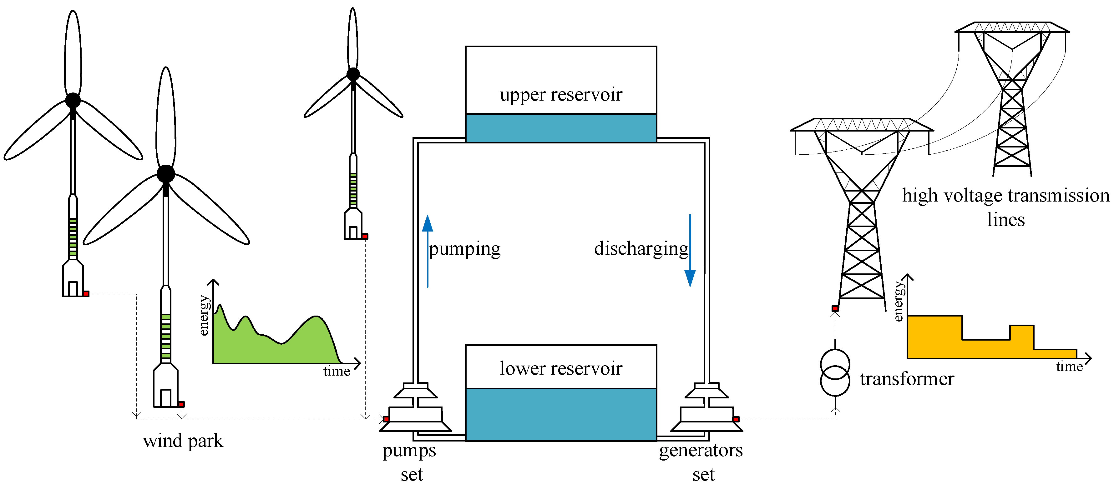
1.1. WT–PSH Hybrid Energy Sources
Scheduling WT–PSH Operation
- Varkani et al. [23] proposed the concept of a self-scheduling strategy which is based on stochastic programming techniques and aims to minimise the impact of wind power generation’s uncertainty. The strategy presented by the authors can be applied for day-ahead energy generation offers. The uncertainty of the wind generation forecasts is modelled by means of an artificial neural network (ANN);
- Tan et al. [24] developed a two-stage scheduling optimisation model for the operation of a wind power and energy storage system based on day-ahead and ultra-short-term wind power forecasting. The results indicate that synergies of demand response and energy storage can be used to overcome wind generation variability and lead to an improvement in utilisation of wind energy, as well as decreasing coal consumption. Similarly, as in [23], the uncertainty of wind power was simulated, in this case being based on a scenario analysis;
- Jurasz and Mikulik [25] suggested a model for scheduling the operation of WT–PSH based on the occupancy of the upper reservoir. It was assumed that the sets of pumps and generators of the PSH can operate simultaneously. The results indicate that WT–PSH operating on such a formula can be a reliable energy source operating as a baseload (with potential modifications regarding when the energy from the upper reservoir should be dispatched). Additionally, the scheduling formula eliminates the occurrence of wind energy rejection. However, the schedule of the WT–PSH operation for the next 1 to 24 h is known only one hour ahead;
- Castronuovo nd Lopes [26] proposed a model for improving wind parks’ operational economic gains by means of PSH facilities. Using an hourly-discretised algorithm the authors identified an optimal daily operation strategy assuming that wind power forecasts were available; and
- Papaefthimiou et al. [27] suggested several possible operation modes for WT–PSH focusing on their verbal description. In general: the WT–PSH can submit an energy offer for the next 24 h considering the state of charge of its upper reservoir; the system operator dispatches the PSH operation mainly during peak load hours or to shave the peaks; the energy generated by the WT is stored in the upper reservoir and the PSH pumps balance the varying WT energy yield—basically, using variable-speed pumps the PSH is able to constantly adjust to the changes in wind generation; the system operator requires the WT–PSH to deliver power in certain periods in order to fill deficits resulting from the limited capacity of the conventional power sources; and the WT–PSH is designed to deliver guaranteed power, but if the upper reservoir state of charge is not sufficient and/or the wind generation forecasts are unfavourable then it is admissible to use electricity from the grid and dispatch it when required. According to their results, the authors state that the proposed operating policies enable the integration of wind generation on a larger scale.
1.2. Wind Speed Forecasting
1.3. WT–PSH
1.4. Paper Objectives
- to develop a MINLP model for simulating the operation of the WT–PSH hybrid and scheduling its operation;
- to establish measures for estimating the model’s accuracy; and
- to investigate the impact of the scheduling formula parameters and upper reservoir capacity on WT–PSH performance.
2. Mathematical Model
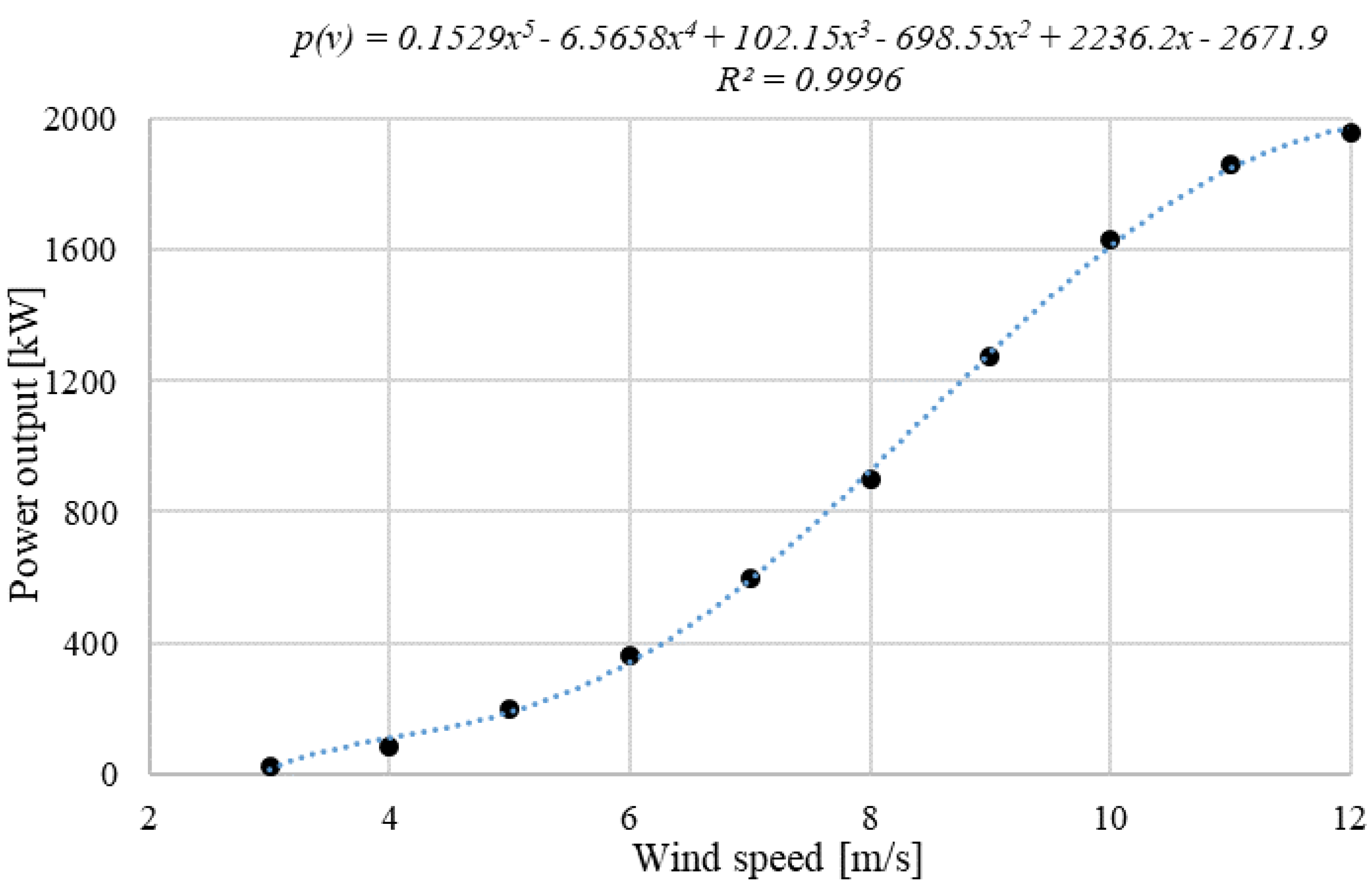
2.1. Energy Yield from Wind Turbines
2.2. WT–PSH Operation
WPSH Operation
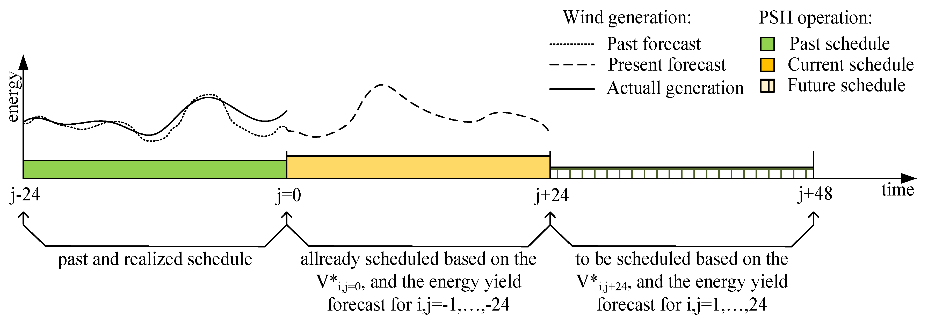
- Step 1.
- Obtain/generate wind turbine energy yield forecast for the next 24 h.
- Step 2.
- Determine the upper reservoir state of filling at the end of the upcoming day (j = 24) based on the already scheduled discharge covering the next 24 h (j = 1, …, 24) and possible energy generation from wind turbines calculated in the first step.
- Step 3.
- Considering the estimated reservoir occupancy of the upper reservoir in step 2, generate a uniform discharge schedule for the next 25 to 48 h (j = 25, …, 48).
- Step 4.
- After realising the previously-planned schedule for the period (j = 1, ..., 24) juxtapose the scheduled and actual operation of the PSH as well as the wind turbine generation and upper reservoir occupancy. In case of any discrepancies replace the estimated occupancy of the upper reservoir calculated in step 2 by the actual one.
- Step 5.
- Return to the step 1 and repeat the whole procedure.
3. Input Data
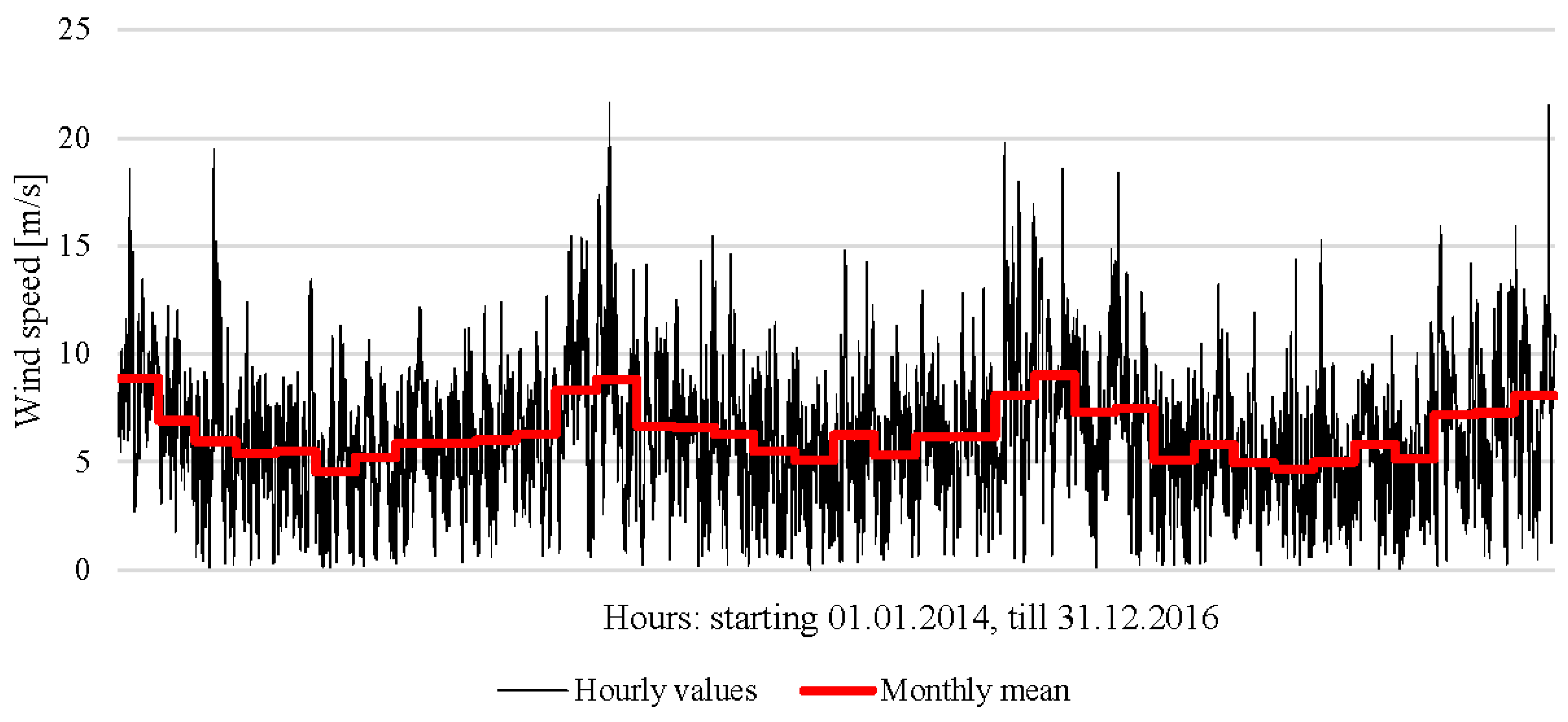
3.1. Wind Data
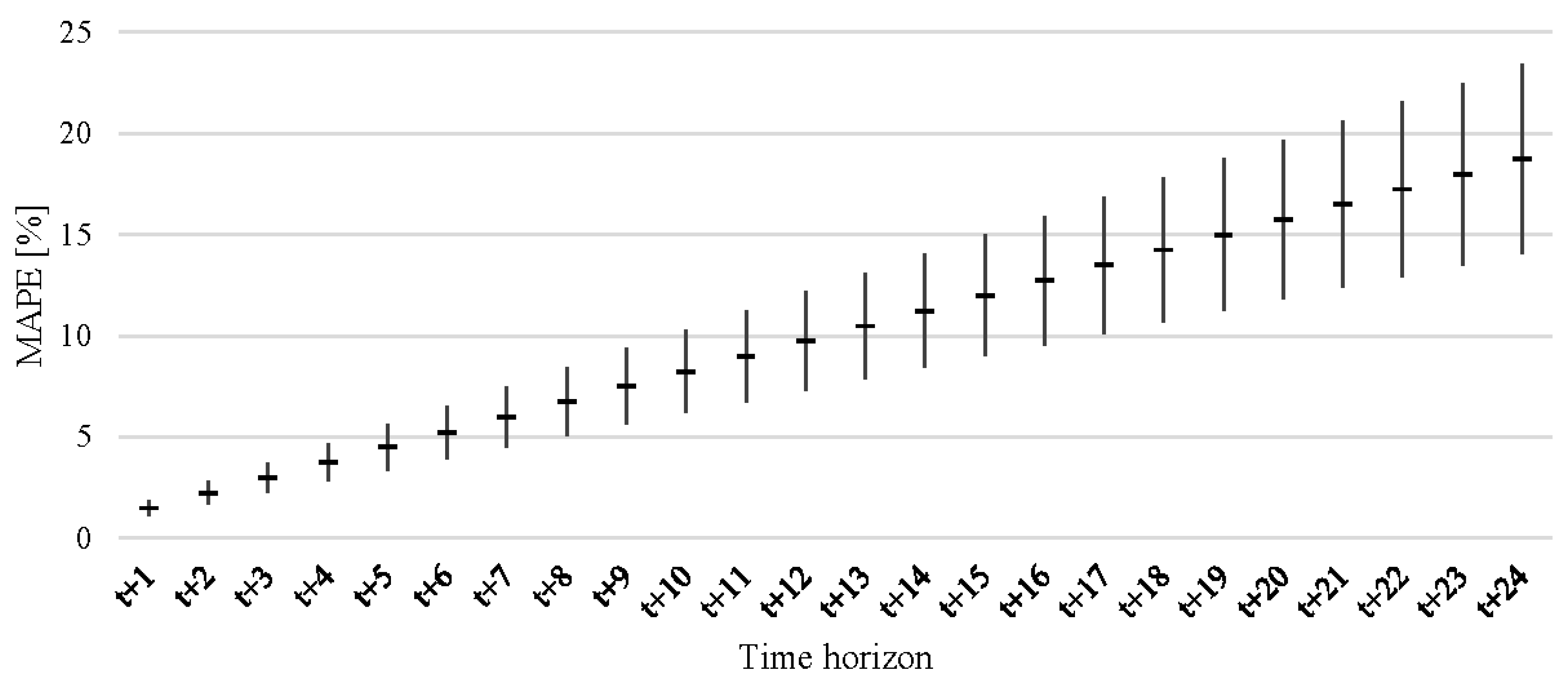
3.2. Wind Speed Forecast Accuracy
3.3. WT-PSH Parameters
4. Results and Discussion
4.1. WT-PSH Parameters
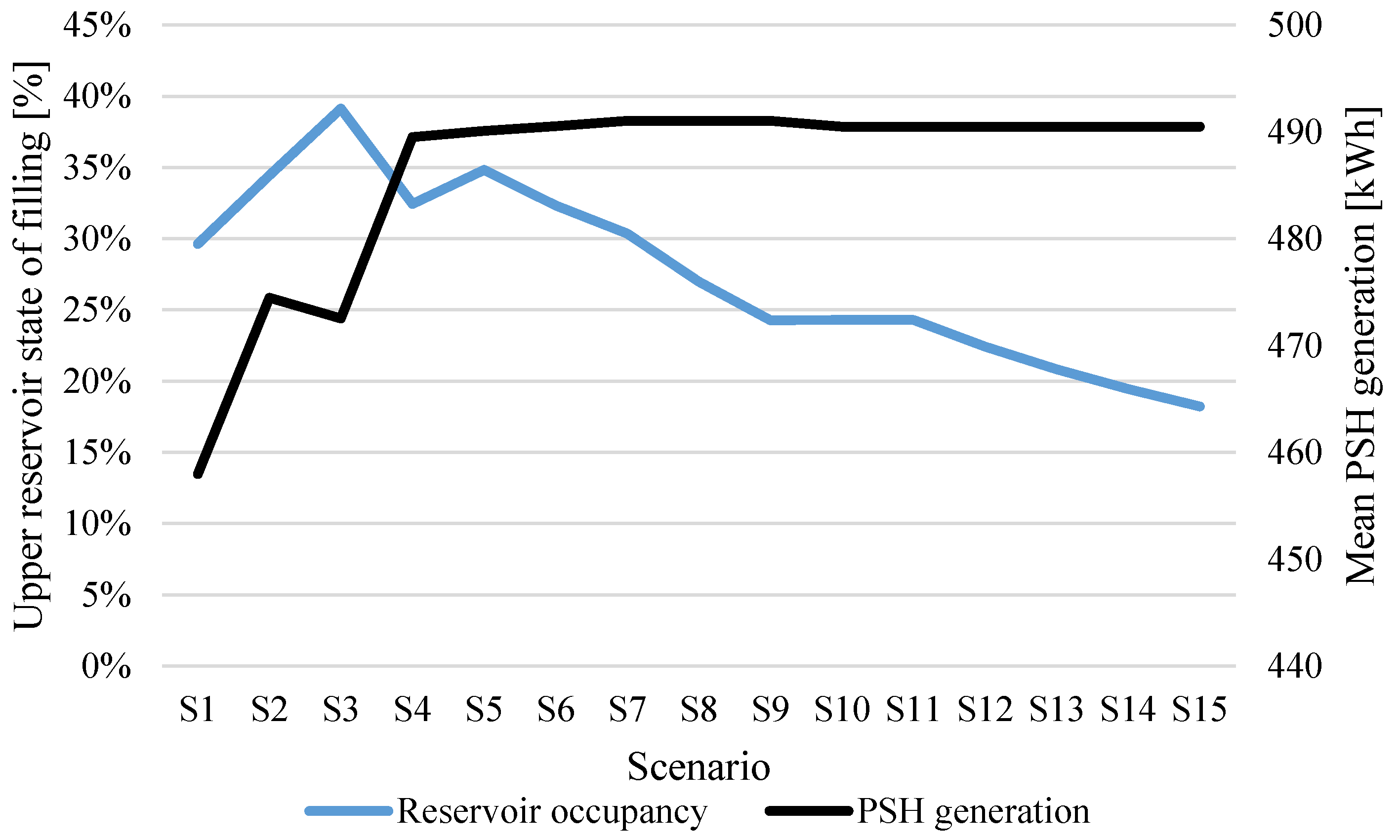
- the unpredictability of the wind generation from 27% (MAPE error for the wind generation forecasts) to less than 1.5% for scenarios S6–S15;
- the hourly variability of the wind generation time series by at least 10%, as in scenarios S2–S9, or almost 23%, as in scenarios S10–S15; and
- the intraday variability from 31% to less than 1%, as in scenarios S5–S10.
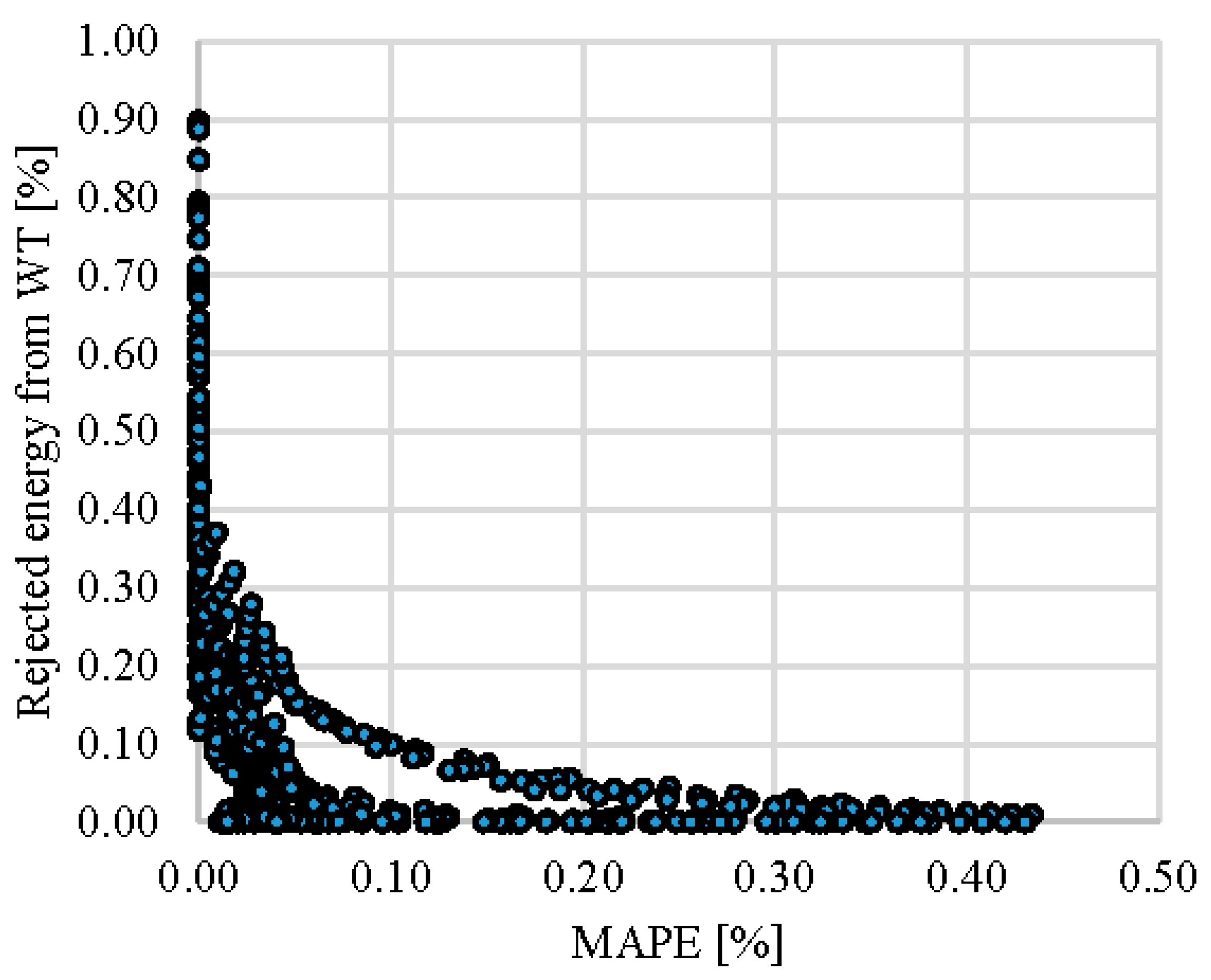
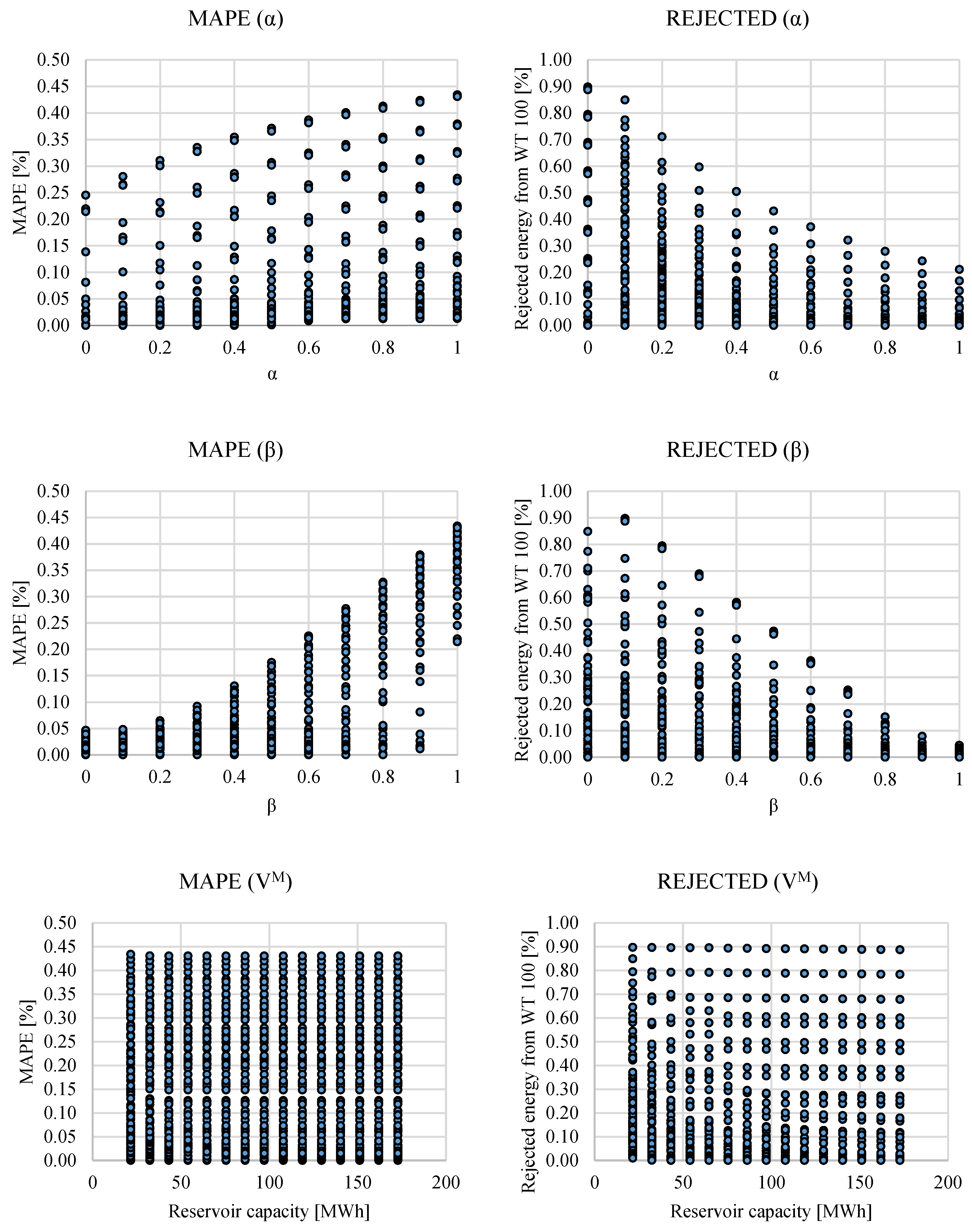
4.2. Sensitivity Analysis
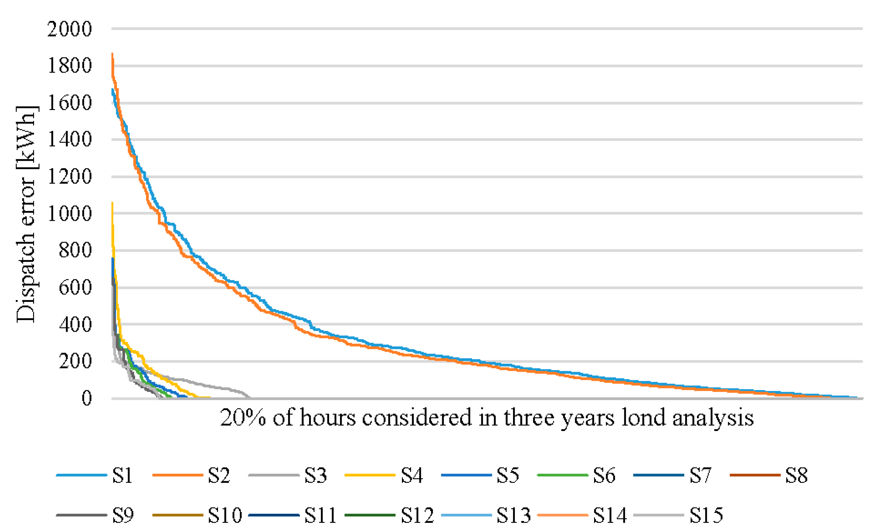
4.3. Analysis of the Dispatch Errors
5. Conclusions
Author Contributions
Funding
Conflicts of Interest
Nomenclature
| Abbreviations | |
| AVG | Average |
| ANN | Artificial Neural Network |
| CAES | Compressed Air Energy Storage |
| CC | Coefficient of Correlation |
| CV | Coefficient of Variation |
| DMS | Demand Side Management |
| NPS | National Power System |
| NWP | Numerical Weather Predictors |
| MAPE | Mean Absolute Percentage Error |
| PSH | Pumped Storage-Hydroelectricity |
| PV | Photovoltaics |
| ROR | Rate of Return |
| STD | Standard Deviation |
| VRES | Variable Renewable Energy Sources |
| V2G | Vehicle to Grid |
| Indexes | |
| i | Index of days (i = 1, …, 1095) |
| j | Index of hours (j = 1, …, 24) |
| Parameters and constants | |
| ηPSH | Efficiency of the PSH pumps and generators (%) |
| EC | Scheduled energy generation of the PSH (kWh) |
| ECR | Scheduled and realised generation of the PSH (kWh) |
| EGen | Maximal energy generating capacity of the PSH per unit of time (kWh) |
| EPump | Maximal capacity of the PSH pumps to accommodate and store the energy in the upper reservoir per unit of time (kWh) |
| EWT | Energy yield from wind turbine (kWh) |
| EWT* | Forecasted energy yield from wind turbine (kWh) |
| EWT_R | Energy yield from wind turbine which has not been used in the PSH generation and/or cannot be stored in the upper reservoir (kWh) |
| n | Number of wind turbines with rated power capacity equal to PWT (-) |
| p(v) | Polynomial approximating the wind turbine power curve (kW) |
| PWT | Rated power output of the selected type of wind turbine (kW) |
| t | Time (hour) |
| v | Wind speed (m/s) |
| v* | Forecasted wind speed (m/s) |
| V | Upper reservoir state of filling (kWh) |
| V* | Estimated/forecasted upper reservoir state of filling (kWh) |
| vcut-in | Wind speed at which wind turbine starts to generate electricity (m/s) |
| vcut-off | Wind speed at which wind turbine operation is interrupted to prevent it being damaged (m/s) |
| vrated | Wind speed at which wind turbine generates electricity at its rated capacity (m/s) |
| Variables | |
| α | Parameter used to define the share of potential wind turbine energy yields used in the PSH generation schedule |
| β | Parameter used to define the contribution of the estimated upper reservoir occupancy to the PSH generation schedule |
| VM | Maximal energy storage capacity of the PSH (kWh) |
References
- Suganthi, L.; Samuel, A.A. Energy models for demand forecasting—A review. Renew. Sustain. Energy Rev. 2014, 16, 1223–1240. [Google Scholar] [CrossRef]
- Jung, J.; Broadwater, R.P. Current status and future advances for wind speed and power forecasting. Renew. Sustain. Energy Rev. 2014, 31, 762–777. [Google Scholar] [CrossRef]
- Kyritsis, E.; Andersson, J.; Serletis, A. Electricity prices, large-scale renewable integration, and policy implications. Energy Policy 2017, 101, 550–560. [Google Scholar] [CrossRef]
- Santos, S.F.; Fitiwi, D.Z.; Cruz, M.R.; Cabrita, C.M.; Catalão, J.P. Impacts of optimal energy storage deployment and network reconfiguration on renewable integration level in distribution systems. Appl. Energy 2017, 185, 44–55. [Google Scholar] [CrossRef]
- Jones, L.E. Renewable Energy Integration: Practical Management of Variability, Uncertainty, and Flexibility in Power Grids; Academic Press: Cambridge, MA, USA, 2014. [Google Scholar]
- Jacobson, M.Z.; Delucchi, M.A. Providing all global energy with wind, water, and solar power, Part I: Technologies, energy resources, quantities and areas of infrastructure, and materials. Energy Policy 2011, 39, 1154–1169. [Google Scholar] [CrossRef]
- Delucchi, M.A.; Jacobson, M.Z. Providing all global energy with wind, water, and solar power, Part II: Reliability, system and transmission costs, and policies. Energy Policy 2011, 39, 1170–1190. [Google Scholar] [CrossRef]
- Kaldellis, J.K.; Kapsali, M.; Kavadias, K.A. Energy balance analysis of wind-based pumped hydro storage systems in remote island electrical networks. Appl. Energy 2010, 87, 2427–2437. [Google Scholar] [CrossRef]
- Kapsali, M.; Kaldellis, J.K. Combining hydro and variable wind power generation by means of pumped-storage under economically viable terms. Appl. Energy 2010, 87, 3475–3485. [Google Scholar] [CrossRef]
- Kapsali, M.; Anagnostopoulos, J.S.; Kaldellis, J.K. Wind powered pumped-hydro storage systems for remote islands: A complete sensitivity analysis based on economic perspectives. Appl. Energy 2012, 99, 430–444. [Google Scholar] [CrossRef]
- Kavadias, K.A.; Kapsali, M.; Kaldellis, J.K. An integrated computational method for the optimum sizing of a wind-based pumped hydro storage system. In Proceedings of the European Wind Energy Conference, Marseille, France, 16–19 March 2009. [Google Scholar]
- Papaefthymiou, S.V.; Papathanassiou, S.A. Optimum sizing of wind-pumped-storage hybrid power stations in island systems. Renew. Energy 2014, 64, 187–196. [Google Scholar] [CrossRef]
- Katsaprakakis, D.A.; Christakis, D.G.; Pavlopoylos, K.; Stamataki, S.; Dimitrelou, I.; Stefanakis, I.; Spanos, P. Introduction of a wind powered pumped storage system in the isolated insular power system of Karpathos–Kasos. Appl. Energy 2012, 97, 38–48. [Google Scholar] [CrossRef]
- Katsaprakakis, D.A. Hybrid power plants in non-interconnected insular systems. Appl. Energy 2016, 164, 268–283. [Google Scholar] [CrossRef]
- Anagnostopoulos, J.S.; Papantonis, D.E. Pumping station design for a pumped-storage wind-hydro power plant. Energy Convers. Manag. 2007, 48, 3009–3017. [Google Scholar] [CrossRef]
- Ma, T.; Yang, H.; Lu, L. Feasibility study and economic analysis of pumped hydro storage and battery storage for a renewable energy powered island. Energy Convers. Manag. 2014, 79, 387–397. [Google Scholar] [CrossRef]
- Ma, T.; Yang, H.; Lu, L.; Peng, J. Pumped storage-based standalone photovoltaic power generation system: Modeling and techno-economic optimization. Appl. Energy 2015, 137, 649–659. [Google Scholar] [CrossRef]
- Ma, T.; Yang, H.; Lu, L.; Peng, J. Optimal design of an autonomous solar–wind-pumped storage power supply system. Appl. Energy 2015, 160, 728–736. [Google Scholar] [CrossRef]
- Hessami, M.A.; Bowly, D.R. Economic feasibility and optimisation of an energy storage system for Portland Wind Farm (Victoria, Australia). Appl. Energy 2011, 88, 2755–2763. [Google Scholar] [CrossRef]
- Hedegaard, K.; Meibom, P. Wind power impacts and electricity storage—A time scale perspective. Renew. Energy 2012, 37, 318–324. [Google Scholar] [CrossRef]
- Canales, F.A.; Beluco, A.; Mendes, C.A.B. A comparative study of a wind hydro hybrid system with water storage capacity: Conventional reservoir or pumped storage plant? J. Energy Storage 2015, 4, 96–105. [Google Scholar] [CrossRef]
- Murage, M.W.; Anderson, C.L. Contribution of pumped hydro storage to integration of wind power in Kenya: An optimal control approach. Renew. Energy 2014, 63, 698–707. [Google Scholar] [CrossRef]
- Varkani, A.K.; Daraeepour, A.; Monsef, H. A new self-scheduling strategy for integrated operation of wind and pumped-storage power plants in power markets. Appl. Energy 2011, 88, 5002–5012. [Google Scholar] [CrossRef]
- Tan, Z.F.; Ju, L.W.; Li, H.H.; Li, J.Y.; Zhang, H.J. A two-stage scheduling optimization model and solution algorithm for wind power and energy storage system considering uncertainty and demand response. Int. J. Electr. Power Energy Syst. 2014, 63, 1057–1069. [Google Scholar] [CrossRef]
- Jurasz, J.; Mikulik, J. Scheduling opearation of wind powered pumped-storage hydroelectricity. In Proceedings of the 13th International Conference on Industrial Logistics, Zakopane, Poland, 28 September–1 October 2016; AGH University of Science and Technology: Kraków, Poland, 2016; pp. 74–83. [Google Scholar]
- Castronuovo, E.D.; Lopes, J.P. On the optimization of the daily operation of a wind-hydro power plant. IEEE Trans. Power Syst. 2004, 19, 1599–1606. [Google Scholar] [CrossRef]
- Papaefthimiou, S.; Karamanou, E.; Papathanassiou, S.; Papadopoulos, M. Operating policies for wind-pumped storage hybrid power stations in island grids. IET Renew. Power Gener. 2009, 3, 293–307. [Google Scholar] [CrossRef]
- Helseth, A.; Gjelsvik, A.; Mo, B.; Linnet, U. A model for optimal scheduling of hydro thermal systems including pumped-storage and wind power. IET Gener. Transm. Distrib. 2013, 7, 1426–1434. [Google Scholar] [CrossRef]
- Soman, S.S.; Zareipour, H.; Malik, O.; Mandal, P. A review of wind power and wind speed forecasting methods with different time horizons. In Proceedings of the North American Power Symposium (NAPS), Arlington, TX, USA, 26–28 September 2010; IEEE: Piscataway, NJ, USA, 2010; pp. 1–8. [Google Scholar]
- Makridakis, S.; Wheelwright, S.C.; Hyndman, R.J. Forecasting Methods and Applications; John Wiley & Sons: Hoboken, NJ, USA, 2008. [Google Scholar]
- Zhao, W.; Wei, Y.M.; Su, Z. One day ahead wind speed forecasting: A resampling-based approach. Appl. Energy 2016, 178, 886–901. [Google Scholar] [CrossRef]
- Dong, L.; Wang, L.; Khahro, S.F.; Gao, S.; Liao, X. Wind power day-ahead prediction with cluster analysis of NWP. Renew. Sustain. Energy Rev. 2016, 60, 1206–1212. [Google Scholar] [CrossRef]
- Azimi, R.; Ghofrani, M.; Ghayekhloo, M. A hybrid wind power forecasting model based on data mining and wavelets analysis. Energy Convers. Manag. 2016, 127, 208–225. [Google Scholar] [CrossRef]
- Miettinen, J.J.; Holttinen, H. Characteristics of day-ahead wind power forecast errors in Nordic countries and benefits of aggregation. Wind Energy 2017, 20, 959–972. [Google Scholar] [CrossRef]
- Korkas, C.D.; Baldi, S.; Michailidis, I.; Kosmatopoulos, E.B. Occupancy-based demand response and thermal comfort optimization in microgrids with renewable energy sources and energy storage. Appl. Energy 2016, 163, 93–104. [Google Scholar] [CrossRef]
- Baldi, S.; Karagevrekis, A.; Michailidis, I.T.; Kosmatopoulos, E.B. Joint energy demand and thermal comfort optimization in photovoltaic-equipped interconnected microgrids. Energy Convers. Manag. 2015, 101, 352–363. [Google Scholar] [CrossRef]
- Jurasz, J.; Mikulik, J.; Krzywda, M.; Ciapała, B.; Janowski, M. Integrating a wind-and solar-powered hybrid to the power system by coupling it with a hydroelectric power station with pumping installation. Energy 2018, 144, 549–563. [Google Scholar] [CrossRef]
- Jurasz, J.; Ciapała, B. Integrating photovoltaics into energy systems by using a run-off-river power plant with pondage to smooth energy exchange with the power gird. Appl. Energy 2017, 198, 21–35. [Google Scholar] [CrossRef]
- Yang, Z.; Liu, P.; Cheng, L.; Wang, H.; Ming, B.; Gong, W. Deriving operating rules for a large-scale hydro-photovoltaic power system using implicit stochastic optimization. J. Clean. Prod. 2018, 195, 562–572. [Google Scholar] [CrossRef]
- Moustris, K.P.; Zafirakis, D.; Alamo, D.H.; Medina, R.N.; Kaldellis, J.K. 24-h Ahead Wind Speed Prediction for the Optimum Operation of Hybrid Power Stations with the Use of Artificial Neural Networks. In Perspectives on Atmospheric Sciences; Springer International Publishing: Basel, Switzerland, 2017; pp. 409–414. [Google Scholar]
- Siemens Gamesa Renewable Energy. Available online: http://www.gamesacorp.com/ (accessed on 20 January 2017).
- Jurasz, J. Modeling and forecasting energy flow between national power grid and a solar–wind–pumped-hydroelectricity (PV–WT–PSH) energy source. Energy Convers. Manag. 2017, 136, 382–394. [Google Scholar] [CrossRef]
- National Aeronautics and Space Administration Goddard Space Flight Center. Available online: https://gmao.gsfc.nasa.gov/reanalysis/MERRA-2/ (accessed on 20 January 2017).


| Scenario | Variables | Mape [%] | CV [%] | |||
|---|---|---|---|---|---|---|
| VM | α | β | Hourly | Intraday | ||
| S1 | 21.6 | 0.2 | 1 | 17.63 | 109.48 | 15.84 |
| S2 | 32.4 | 0.1 | 1 | 4.85 | 90.78 | 2.31 |
| S3 | 43.2 | 0.3 | 1 | 3.20 | 90.05 | 1.86 |
| S4 | 54.0 | 0.1 | 1 | 2.39 | 90.02 | 1.15 |
| S5 | 64.8 | 0.9 | 0 | 1.73 | 88.36 | 0.76 |
| S6 | 75.6 | 0.9 | 0 | 1.37 | 88.22 | 0.61 |
| S7 | 86.4 | 0.9 | 0 | 1.15 | 88.05 | 0.43 |
| S8 | 97.2 | 0.9 | 0 | 1.15 | 88.05 | 0.43 |
| S9 | 108.0 | 0.9 | 0 | 1.15 | 88.05 | 0.43 |
| S10 | 118.8 | 0.7 | 0.1 | 1.10 | 78.37 | 0.27 |
| S11 | 129.6 | 0.7 | 0.1 | 1.10 | 78.37 | 0.27 |
| S12 | 140.4 | 0.7 | 0.1 | 1.10 | 78.37 | 0.27 |
| S13 | 151.2 | 0.7 | 0.1 | 1.10 | 78.37 | 0.27 |
| S14 | 162.0 | 0.7 | 0.1 | 1.10 | 78.37 | 0.27 |
| S15 | 172.8 | 0.7 | 0.1 | 1.10 | 78.37 | 0.27 |
| MAPE | Rejected | |
|---|---|---|
| α | 0.3915 | −0.5186 |
| β | 0.8456 | −0.3568 |
| VM | −0.0215 | −0.1545 |
| Scenario | S1 | S2 | S3 | S4 | S5 | S6 | S7–S9 | S10–S15 |
|---|---|---|---|---|---|---|---|---|
| AVG (kWh) | 61.3 | 57.1 | 4.0 | 4.2 | 2.8 | 2.3 | 1.8 | 1.5 |
| STD (kWh) | 199.3 | 191.7 | 25.9 | 38.3 | 28.0 | 25.4 | 23.0 | 16.2 |
| CV [%] | 30.7% | 29.8% | 15.5% | 10.8% | 10.0% | 9.2% | 8.0% | 9.2% |
| Skeweness | 4.6 | 4.9 | 9.4 | 14.0 | 14.7 | 15.1 | 17.9 | 14.8 |
| Kurtosis | 23.7 | 27.5 | 123.1 | 250.1 | 272.7 | 280.1 | 390.7 | 285.7 |
© 2018 by the authors. Licensee MDPI, Basel, Switzerland. This article is an open access article distributed under the terms and conditions of the Creative Commons Attribution (CC BY) license (http://creativecommons.org/licenses/by/4.0/).
Share and Cite
Jurasz, J.; Kies, A. Day-Ahead Probabilistic Model for Scheduling the Operation of a Wind Pumped-Storage Hybrid Power Station: Overcoming Forecasting Errors to Ensure Reliability of Supply to the Grid. Sustainability 2018, 10, 1989. https://doi.org/10.3390/su10061989
Jurasz J, Kies A. Day-Ahead Probabilistic Model for Scheduling the Operation of a Wind Pumped-Storage Hybrid Power Station: Overcoming Forecasting Errors to Ensure Reliability of Supply to the Grid. Sustainability. 2018; 10(6):1989. https://doi.org/10.3390/su10061989
Chicago/Turabian StyleJurasz, Jakub, and Alexander Kies. 2018. "Day-Ahead Probabilistic Model for Scheduling the Operation of a Wind Pumped-Storage Hybrid Power Station: Overcoming Forecasting Errors to Ensure Reliability of Supply to the Grid" Sustainability 10, no. 6: 1989. https://doi.org/10.3390/su10061989
APA StyleJurasz, J., & Kies, A. (2018). Day-Ahead Probabilistic Model for Scheduling the Operation of a Wind Pumped-Storage Hybrid Power Station: Overcoming Forecasting Errors to Ensure Reliability of Supply to the Grid. Sustainability, 10(6), 1989. https://doi.org/10.3390/su10061989