A Game Theoretic Approach for Improving Environmental and Economic Performance in a Dual-Channel Green Supply Chain

Abstract

In this paper, we investigate economic performance and environmental performance of a dual-channel green supply chain (GSC). Given that most relevant literature still focus on the descriptive aspect of GSC, we adopt game theoretic approach rather than qualitative analysis method to address the following problems: (1) How can the integration of environmental and economic sustainability goals be achieved in GSC? (2) What is the impact of customer environmental awareness on the green level and profitability of the GSC? (3) How does the market demand changes in the presence of the online direct channel in addition to the traditional one? We establish four game models, which are decentralized scenario, centralized scenario, retailer-led revenue-sharing scenario and bargaining revenue-sharing scenario. In the decentralized scenario, participants in a GSC make individual decisions based on their specific interests. In the centralized scenario, the GSC is regarded as a whole and the participants make collective decisions to maximize the overall profit of the GSC. In addition, in the two revenue-sharing scenarios, revenue-sharing contracts as the important profit coordination systems are set up and the revenue-sharing ratio is determined either by the retailer or through bargaining. Moreover, the cost of green product research and development, customer environmental awareness and price sensitivity are also taken into account in the four scenarios. By comparing and analyzing the four game models, we recommend the two revenue-sharing scenarios as the optimum choice and improving green awareness as a feasible strategy to achieve the integration of economic and environmental goals of the GSC. Additionally, we find that online sales has become a major distribution channel of the GSC.

1. Introduction

Human activities have to a large extent changed the functioning of the planetary systems [1]. In order to curb the ecological deterioration, sustainable development strategy should be implemented [2]. With regard to corporate sustainability, the lens is beginning to be widened from a specific company to the entire supply chain (SC) [3]. In addition, the impact on environment as well as resource use efficiency need to be considered at the level of supply chain management (SCM) rather than within the boundary of a company [4]. Consequently, the concept of green supply chain (GSC) was proposed and has gained rapidly growing attention from both academia and industry [5].

In contrast to traditional SCM, which typically focuses on economic performance, green supply chain management (GSCM) aims at the integration of environmental and economic sustainability [6]. However, there is still conflicting viewpoints on whether such integrated goals could be achieved [7]. Some researchers claim that the environmental improvement does not always lead to profitability and sometimes may conflict with the economic goal [8]. On the other hand, some researchers argue that GSCM practices may improve a company’s economic performance [9]. These indicate that advancing the green level of the GSC has both negative and positive impacts on economic performance [10]. Nevertheless, turning a blind eye to environmental issues is no longer an option for a company, and GSCM is thus an indispensable requirement [11].

Moreover, customer purchasing behavior has become an important factor affecting the GSCM implementation with the tremendous increase of global consumption [12]. Many investigations indicate that more customers than ever have shown their environmental concerns and desires to purchase green products [13]. However, there is a gap between consumers’ positive attitudes and actual actions, and green consciousness does not always lead to green purchasing behavior [14]. In addition, rapid development of the Internet has significantly changed customer purchasing behavior and the structure of GSC distribution [15]. The rise of online shopping prompts manufacturers to adopt dual-channel strategy, which may expand market share, reduce costs and increase profits [16].

Motivated by everything mentioned above, we investigate the alignment issues between environmental and economic performance of GSC. Previous research mainly focused on description, case study, survey and other empirical methods. In this paper, we adopt game theoretic approach rather than qualitative analysis to answer the following questions:

(1)

How can the integration of environmental and economic sustainability goals be achieved in GSCM?

(2)

What is the impact of customer environmental awareness on the green level and the profitability of the GSC?

(3)

How does the market demand change in the presence of the online direct channel in addition to the traditional one?

In the process of problem-solving, we establish four game models based on a dual-distribution GSC: (i) decentralized scenario where the manufacturer and the retailer of the GSC make decisions independently based on their own interests; (ii) centralized scenario where the GSC is treated as a whole and the manufacturer and the retailer make collective decisions to maximize the overall profit of the GSC; (iii) retailer-led revenue-sharing scenario where the profit coordination mechanisms are set up and the retailer determines the revenue-sharing ratio; (iv) bargaining revenue-sharing scenario where the manufacturer and the retailer determine the revenue-sharing ratio through bargaining in the profit coordination mechanisms. Moreover, the cost of green product research and development (R&D), customer environmental awareness and price sensitivity are also taken into account in the four scenarios.

The main contributions of this paper are presented as follows. First, a game theoretic approach is adopted, and the equilibrium solutions are calculated in four different scenarios. Second, environmental and economic performances in the four scenarios are compared and analyzed to help make decisions in GSCM practice. Third, we assume that the manufacturer can sell green products to customers through both the online direct channel and the traditional channel. Finally, factors such as green product R&D cost, customer green sensitivity and price sensitivity, which affect the green level and profitability of GSCM, are taken into account.

The rest of the paper is organized into six sections. In Section 2, a brief review of relevant literature is provided. In Section 3, the problem structure is described and four game models are introduced. In Section 4, the optimal solutions of the four scenarios are acquired. In Section 5, the four game models are compared and analyzed. Section 6 provides a numerical example to illustrate the sensitivity of the optimal solutions to some parameters. Finally, conclusions and future research directions are outlined in Section 7.

2. Literature Review

SC is a vertical sequence of independent transactions, which can be viewed as a flow of material, products and information and a set of corporate activities [17]. It is not surprising that corporate sustainable strategies have been extended through the SC for the broader adoption and development of sustainability [3]. GSCM is an effective management tool and philosophy to embed environmental sustainability into SCM [18]. In addition, many activities are involved in GSCM, such as green product design, materials acquisition, green manufacturing processes, distribution, use, and resource recycling [19]. However, the scope of GSCM in the literature has varied according to the goal of the investigator [20]. In this paper, we shall focus on the manufacturer-retailer-customer relationship and pertinent activities of green production, green marketing and green purchasing in the dual-channel structure.

Environmental and economic performances of GSM have been a topic of intense interest in GSCM literature, where both positive and negative relations between the two performances are observed. As for research methods, survey research and case study are dominant and thus most relevant literature still concentrate on the qualitative aspect of GSCM [21]. In addition, many of the related studies are criticized for lacking in long term results and helping make decisions in GSCM [22]. In this paper, we use quantitative analysis method and provide insights on the effects of factors such as green production, sale channel and green customer on the green level and profitability of GSCM.

Given that better planning and coordination of GSCM practices can generate positive environmental and economic effects, some researchers developed mathematical models to assess the impacts of decision-making and operation of GSC players [23]. Moreover, corporate approaches for performance improvement cannot be undertaken in isolation, so a concerted effort along GSC players is needed [24]. On the other hand, with different profit targets and operation strategies, GSC players can hardly maintain consistency on everything, and sometimes they are in competition with one another. Among all the mathematical methods used in GSCM literature, game theory is highly applicable to the research on the coexistence of competition and cooperation among GSC players.

In the field of GSC logistics, game theory is applied not only to forward logistics but also to reverse logistics whose function are recycling, reusing, and remanufacturing. As a forward logistics example, Barari et al. [25] studied the coordination between the manufacturer and the retailer in an evolutionary game model. They found such coordination could increase environmental benefits and commercial advantages of GSC. As a reverse logistics example, Sheu and Chen [26] applied a three-stage game model to a GSC with both forward and reverse logistics. In addition, low-wholesale-price strategies are suggested for recycling processes under government green subsidization. In this paper, our scope covers only forward logistics of GSC.

We categorize the coexistence of competition and cooperation of GSC players into types of chain and chain, channel and channel, upstream and downstream companies. Jamali and Rasti-Barzoki [12] studied the chain-chain competition of two dual-channel SCs under centralized and decentralized scenarios. They found that the centralized scenario achieves a higher green level of production than the decentralized one does. Chen et al. [27] investigated duopoly GSC with upstream-downstream and channel-channel competition. They explored how manufacturers’ market power influences the pricing policies and green strategies. Ghosh and Shah [28] explored the effect of decentralized policy and cooperative policy on the green level of products in a secondary SC composed of a manufacturer and a retailer. The green level is decided individually by the manufacturer in the decentralized policy, while cooperative decisions are made between the upstream and downstream players in the cooperative policy. Then they further put forward a contractual coordination mechanism. In this paper, we focus on the competition and cooperation of channel-channel and upstream-downstream types.

There are many application aspects of game theory to GSCM, such as R&D collaboration, governmental intervention and pricing policy. Dai et al. [29] established Stackleberg game models to study R&D collaboration between GSC members. They revealed that the upstream company generally prefers a Cartelization, while the downstream company mostly favors a non-cooperative scheme. In addition, the Cost-sharing contract generally makes the chain-wide profit get to the summit. Yang and Xiao [30] used game method to explore the governmental interventions in a GSC. They found that with the increase of governmental interventions, the green level of GSC will increase. However, a relatively high green level floor for subsidy causes the first-mover disadvantage of manufacturers. Wei et al. [31] studied the pricing problem in the GSC comprised of two manufacturers and one retailer. In view of the manufacturers’ cooperation or noncooperation strategies, they adopted the centralized models and decentralized models. In this paper, we regard prices as decision variables in our game models.

3. Problem Statement and Formulation

3.1. Problem Description

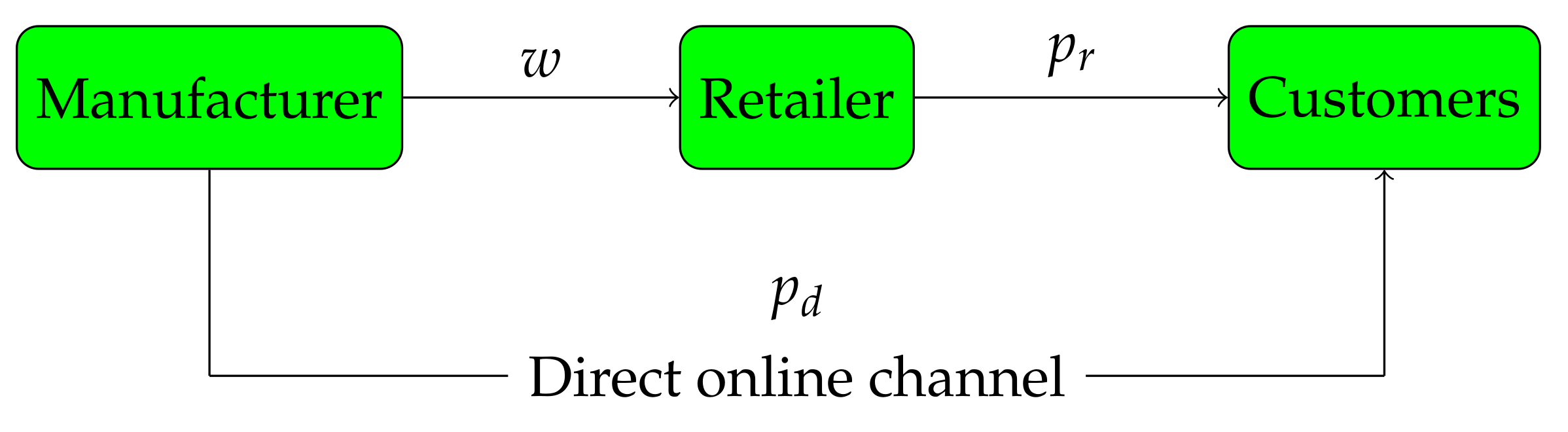
In this paper, we investigate the alignment issues between green level and economic performance of GSC. We are particularly interested to see how the alignment may be achieved through competition and cooperation of the GSC participants. To answer this question, we take into account a dual-distribution GSC composed of a manufacturer, a retailer and customers, as shown in Figure 1. The manufacturer produces green products, which are sold to customers through a retailer or a direct channel. Based on this, four game models are established. Moreover, the effects of green product R&D cost, customer green sensitivity and price sensitivity, are evaluated into the above models by using corresponding coefficients.

3.2. Notation

We collect model parameters and decision variables which are used in the four game models. The notations and meanings of them are listed in

Table 1. Model parameters and decision variables.

Model Parameter
D	the market’s total potential demand
$D_1$	the demand in the traditional retail channel
$D_2$	the demand in the direct channel
$c_m$	uint production cost of the green product
$\alpha$	self-price sensitivity coefficient
$\beta$	cross-price sensitivity coefficient
r	green sensitivity coefficient
i	green investment coefficient
Decision Variable
$\theta$	green degree of the green product
w	wholesale price of the green product
$p_r$	retail price of the green product
$p_d$	direct price of the green product

.

3.3. Assumptions

We make the following assumptions, where the parameters and variables are shown in Table 1.

(1)

$p_r>w>c_m$. In order to ensure profits for the retailer and the manufacturer, the retail price must be higher than the wholesale price, and the wholesale price higher than the production cost.

(2)

$\alpha >\beta >0$. This indicates that the customers of a given channel are more sensitive to the price changes in this channel than that in the other channel. This assumption is made in many studies, for instance literature [12].

(3)

To advance green product R&D, manufacturers need to invest a lot of funds. In addition, the R&D cost is assumed as $i{\theta }^2$. This type of cost function is considered in many studies, for instance literature [27].

(4)

The demand functions of green product in traditional sale channel and online direct channel are as follows, respectively.

$$D_1=D-\alpha p_r+\beta p_d+r\theta$$

(1)

$$D_2=D-\alpha p_d+\beta p_r+r\theta$$

(2)

3.4. The Profit Functions for Each Player

Based on the above assumptions, the manufacturer’s profit function is:

$${\pi }_m=(w-c_m)D_1+(p_d-c_m)D_2-i{\theta }^2$$

(3)

The retailer’s profit function is:

$${\pi }_r=(p_r-w)D_1$$

(4)

The total profit function for the supply chain is:

$${\pi }_{sc}=(p_r-c_m)D_1+(p_d-c_m)D_2-i{\theta }^2$$

(5)

4. The Model

4.1. Decentralized Scenario

In the decentralized scenario, Stackelberg competition between the manufacturer and the retailer is established. As the leader of the competition, the manufacturer determines the green degree of the product, the wholesale price and the direct price; then, the retailer determines the product’s retail price correspondingly. The model is formulated as:

$$\left\{\begin{array}{c}max{\pi }_m=(w-c_m)D_1+(p_d-c_m)D_2-i{\theta }^2\hfill \\ s.t.max{\pi }_r=(p_r-w)D_1\hfill \end{array}\right.$$

(6)

Theorem 1.

In the decentralized scenario, the optimal green degree, wholesale price, retail price, and direct price are given as follows:

$${\theta }^{M^{*}}={\displaystyle \frac{r(3\alpha +\beta )(D-\alpha c_m+\beta c_m)}{8{\alpha }^{2}i-3\alpha r^2-8\alpha \beta i-\beta r^2}}$$

(7)

$$w^{M^{*}}={\displaystyle \frac{3\alpha r^2{c}_m-4{\alpha }^{2}i{c}_m-4\alpha iD+\beta r^2{c}_m+4\alpha \beta i{c}_m}{3\alpha r^2+8\alpha \beta i+\beta r^2-8{\alpha }^{2}i}}$$

(8)

$$p_r^{M^{*}}={\displaystyle \frac{3\alpha r^2{c}_m-2{\alpha }^{2}i{c}_m-6\alpha iD+2{\beta }^{2}i{c}_m+\beta r^2{c}_m+2\beta iD}{3\alpha r^2+8\alpha \beta i+\beta r^2-8{\alpha }^{2}i}}$$

(9)

$$p_d^{M^{*}}={\displaystyle \frac{3\alpha r^2{c}_m-4{\alpha }^{2}i{c}_m-4\alpha iD+\beta r^2{c}_m+4\alpha \beta i{c}_m}{3\alpha r^2+8\alpha \beta i+\beta r^2-8{\alpha }^{2}i}}$$

(10)

and the profits of the manufacturer, the retailer and the overall GSC are respectively:

$${\pi }_m^{M^{*}}={\displaystyle \frac{-i(3\alpha +\beta ){(D-\alpha c_m+\beta c_m)}^2}{3\alpha r^2+8\alpha \beta i+\beta r^2-8{\alpha }^{2}i}}$$

(11)

$${\pi }_r^{M^{*}}={\displaystyle \frac{4\alpha i^2{(\alpha -\beta )}^2{(D-\alpha c_m+\beta c_m)}^2}{{(3\alpha r^2+8\alpha \beta i+\beta r^2-8{\alpha }^{2}i)}^2}}$$

(12)

$${\pi }_{sc}^{M^{*}}={\displaystyle \frac{i{(D-\alpha c_m+\beta c_m)}^{2}A}{{(3\alpha r^2+8\alpha \beta i+\beta r^2-8{\alpha }^{2}i)}^2}}$$

(13)

The value of A is shown in Appendix A, and the proof of Theorem 1 appears in Appendix B.

4.2. Centralized Scenario

In the centralized scenario, the GSC is regarded as a whole. Instead of making decisions based on their own interests, the manufacturer and the retailer make collective decisions to maximize the overall profits of the GSC. As a result, a high requirement is set for the decision-makers. The model is formulated as:

$$max{\pi }_{sc}=(p_r-c_m)D_1+(p_d-c_m)D_2-i{\theta }^2$$

(14)

Theorem 2.

In the centralized scenario, the optimal green degree, retail price, direct price and the overall profit of the GSC are given as follows:

$${\theta }^{*}={\displaystyle \frac{r(D-\alpha c_m+\beta c_m)}{2\alpha i-r^2-2\beta i}}$$

(15)

$$p_r^{*}={\displaystyle \frac{Di+\alpha c_{m}i-r^2{c}_m-\beta c_{m}i}{2\alpha i-r^2-2\beta i}}$$

(16)

$$p_d^{*}={\displaystyle \frac{Di+\alpha c_{m}i-r^2{c}_m-\beta c_{m}i}{2\alpha i-r^2-2\beta i}}$$

(17)

$${\pi }_{sc}^{*}={\displaystyle \frac{i{(D-\alpha c_m+\beta c_m)}^2}{2\alpha i-r^2-2\beta i}}$$

(18)

The proof of Theorem 2 appears in Appendix B.

4.3. Revenue-Sharing Scenario

In this section, we establish a retailer-led revenue-sharing contract game model and a bargaining revenue-sharing contract game model. In order to advance the green level of the SC, the profit coordination systems are set up in both models to reduce the manufacturer’s burden of the green product R&D. That is, the retailer will return a share of retail profits to the manufacturer. The percentage of retailer gain from retail profits is $\lambda (0<\lambda <1)$, and the percentage of manufacturer gain from retail profits is $1-\lambda$.

4.3.1. Retailer-Led Revenue-Sharing Scenario

In this model, the retailer determines the revenue-sharing ratio $\lambda$. The manufacturer determines the wholesale price, the price and the green degree, and then the retailer determines the retail price according to the manufacturer’s decision. The model is formulated as:

$$\left\{\begin{array}{c}max{\pi }_r=\lambda (p_r-w)D_1\hfill \\ s.t.max{\pi }_m=(w-c_m)D_1+(p_d-c_m)D_2-i{\theta }^2+(1-\lambda )(p_r-w)D_1\hfill \end{array}\right.$$

(19)

Theorem 3.

In the retailer-led revenue-sharing scenario, the optimal revenue-sharing ratio, green degree, wholesale price, retail price and direct price are:

$${\lambda }^{R^{*}}={\displaystyle \frac{4\alpha \beta i+2\alpha r^2-4{\alpha }^{2}i}{4\alpha \beta i+\alpha r^2+\beta r^2-4{\alpha }^{2}i}}$$

(20)

$${\theta }^{R^{*}}={\displaystyle \frac{r(D-\alpha c_m+\beta c_m)(3{\alpha }^{2}i-2\alpha \beta i-\alpha r^2-{\beta }^{2}i-\beta r^2)}{B}}$$

(21)

$$w^{R^{*}}={\displaystyle \frac{C{c}_m+(8{\alpha }^3{i}^2-8{\alpha }^2\beta i^2-4{\alpha }^2{r}^{2}i+\alpha \beta r^{2}i-{\beta }^2{r}^{2}i)D}{2\alpha B}}$$

(22)

$$p_r^{R^{*}}={\displaystyle \frac{E{c}_m+(12{\alpha }^2{i}^2-16\alpha \beta i^2-5\alpha r^{2}i+4{\beta }^2{i}^2+\beta r^{2}i)D}{2B}}$$

(23)

$$p_d^{R^{*}}={\displaystyle \frac{F{c}_m+(8{\alpha }^2{i}^2-8\alpha \beta i^2-3\alpha r^{2}i-\beta r^{2}i)D}{2B}}$$

(24)

and the profits of the manufacturer, the retailer and the total supply chain are respectively:

$${\pi }_m^{R^{*}}={\displaystyle \frac{(D-\alpha c_m+\beta c_m)(3{\alpha }^{2}i-2\alpha \beta i-\alpha r^2-{\beta }^{2}i-\beta r^2)}{B}}$$

(25)

$${\pi }_r^{R^{*}}={\displaystyle \frac{i^2{(\alpha -\beta )}^2{(D-\alpha c_m+\beta c_m)}^2}{2(r^2-2\alpha i+2\beta i)(\alpha r^2+\beta r^2+4\alpha \beta i-4{\alpha }^{2}i)}}$$

(26)

$${\pi }_{sc}^{R^{*}}={\displaystyle \frac{i{(D-\alpha c_m+\beta c_m)}^2(7{\alpha }^{2}i-6\alpha \beta i-2\alpha r^2-{\beta }^{2}i-2\beta r^2)}{2B}}$$

(27)

The values of B, C, E and F are shown in Appendix A, and the proof of Theorem 3 appears in Appendix B.

4.3.2. Bargaining Revenue-Sharing Scenario

In this model, the revenue-sharing ratio $\lambda$ is determined by the manufacturer and the retailer through bargaining rather than determined by the retailer. The model is formulated as:

$$max{\pi }_B={\pi }_m{\pi }_r$$

(28)

Theorem 4.

In the bargaining revenue-sharing scenario, the optimal revenue-sharing ratio, green degree, wholesale price, retail price and direct price are:

$${\lambda }^{B^{*}}={\displaystyle \frac{2\alpha \beta i+\alpha r^2-2{\alpha }^{2}i}{4\alpha \beta i+\alpha r^2+\beta r^2-4{\alpha }^{2}i}}$$

(29)

$${\theta }^{B^{*}}={\displaystyle \frac{r(D-\alpha c_m+\beta c_m)(10{\alpha }^{2}i-8\alpha \beta i-3\alpha r^2-2{\beta }^{2}i-3\beta r^2)}{3B}}$$

(30)

$$w^{B*}={\displaystyle \frac{A_1{c}_m+(4{\alpha }^2\beta i^2-8{\alpha }^3{i}^2+4{\alpha }^2{r}^{2}i+4\alpha {\beta }^2{i}^2+2{\beta }^2{r}^{2}i)D}{3\alpha B}}$$

(31)

$$p_r^{B^{*}}={\displaystyle \frac{B_1{c}_m+(16{\alpha }^2{i}^2-20\alpha \beta i^2-6\alpha r^{2}i+4{\beta }^2{i}^2)D}{2B}}$$

(32)

$$p_d^{B^{*}}={\displaystyle \frac{C_1{c}_m+(12{\alpha }^2{i}^2-12\alpha \beta i^2-4\alpha r^{2}i-2\beta r^2{i}^2)D}{2B}}$$

(33)

and the profits of and the profits of the manufacturer, the retailer and the total supply chain are respectively:

$${\pi }_m^{B^{*}}={\displaystyle \frac{i{(D-\alpha c_m+\beta c_m)}^2(10{\alpha }^{2}i-8\alpha \beta i-3\alpha r^2-2{\beta }^{2}i-3\beta r^2)}{3B}}$$

(34)

$${\pi }_r^{B^{*}}={\displaystyle \frac{4i^2{(\alpha -\beta )}^2{(D-\alpha c_m+\beta c_m)}^2}{9(r^2-2\alpha i+2\beta i)(\alpha r^2+\beta r^2+4\alpha \beta i-4{\alpha }^{2}i)}}$$

(35)

$${\pi }_{sc}^{B^{*}}={\displaystyle \frac{i{(D-\alpha c_m+\beta c_m)}^2(34{\alpha }^{2}i-32\alpha \beta i-9\alpha r^2-2{\beta }^{2}i-9\beta r^2)}{9B}}$$

(36)

The values of $A_1$, $B_1$ and $C_1$ are shown in Appendix A, and the proof of Theorem 4 appears in Appendix B.

5. Model Comparison

Equilibrium solutions of the four models are shown in

Table 2. Equilibrium solutions.

	Decentralized Scenario	Centralized Scenario	Retailer-Led Revenue-Sharing	Bargaining Revenue-Sharing
$\lambda$	−	−	${\displaystyle \frac{4\alpha \beta i+2\alpha r^2-4{\alpha }^{2}i}{4\alpha \beta i+\alpha r^2+\beta r^2-4{\alpha }^{2}i}}$	${\displaystyle \frac{2\alpha \beta i+\alpha r^2-2{\alpha }^{2}i}{4\alpha \beta i+\alpha r^2+\beta r^2-4{\alpha }^{2}i}}$
$\theta$	${\displaystyle \frac{r(3\alpha +\beta )(D-\alpha c_m+\beta c_m)}{8{\alpha }^{2}i-3\alpha r^2-8\alpha \beta i-\beta r^2}}$	${\displaystyle \frac{r(D-\alpha c_m+\beta c_m)}{2\alpha i-r^2-2\beta i}}$	${\displaystyle \frac{r(D-\alpha c_m+\beta c_m)(3{\alpha }^{2}i-2\alpha \beta i-\alpha r^2-{\beta }^{2}i-\beta r^2)}{B}}$	${\displaystyle \frac{r(D-\alpha c_m+\beta c_m)(10{\alpha }^{2}i-8\alpha \beta i-3\alpha r^2-2{\beta }^{2}i-3\beta r^2)}{3B}}$
w	${\displaystyle \frac{3\alpha r^2{c}_m-4{\alpha }^{2}i{c}_m-4\alpha iD+\beta r^2{c}_m+4\alpha \beta i{c}_m}{3\alpha r^2+8\alpha \beta i+\beta r^2-8{\alpha }^{2}i}}$	−	${\displaystyle \frac{C{c}_m+(8{\alpha }^3{i}^2-8{\alpha }^2\beta i^2-4{\alpha }^2{r}^{2}i+\alpha \beta r^{2}i-{\beta }^2{r}^{2}i)D}{2\alpha B}}$	${\displaystyle \frac{A_1{c}_m+(4{\alpha }^2\beta i^2-8{\alpha }^3{i}^2+4{\alpha }^2{r}^{2}i+4\alpha {\beta }^2{i}^2+2{\beta }^2{r}^{2}i)D}{3\alpha B}}$
$p_r$	${\displaystyle \frac{3\alpha r^2{c}_m-2{\alpha }^{2}i{c}_m-6\alpha iD+2{\beta }^{2}i{c}_m+\beta r^2{c}_m+2\beta iD}{3\alpha r^2+8\alpha \beta i+\beta r^2-8{\alpha }^{2}i}}$	${\displaystyle \frac{Di+\alpha c_{m}i-r^2{c}_m-\beta c_{m}i}{2\alpha i-r^2-2\beta i}}$	${\displaystyle \frac{E{c}_m+(12{\alpha }^2{i}^2-16\alpha \beta i^2-5\alpha r^{2}i+4{\beta }^2{i}^2+\beta r^{2}i)D}{2B}}$	${\displaystyle \frac{B_1{c}_m+(16{\alpha }^2{i}^2-20\alpha \beta i^2-6\alpha r^{2}i+4{\beta }^2{i}^2)D}{2B}}$
$p_d$	${\displaystyle \frac{3\alpha r^2{c}_m-4{\alpha }^{2}i{c}_m-4\alpha iD+\beta r^2{c}_m+4\alpha \beta i{c}_m}{3\alpha r^2+8\alpha \beta i+\beta r^2-8{\alpha }^{2}i}}$	${\displaystyle \frac{Di+\alpha c_{m}i-r^2{c}_m-\beta c_{m}i}{2\alpha i-r^2-2\beta i}}$	${\displaystyle \frac{F{c}_m+(8{\alpha }^2{i}^2-8\alpha \beta i^2-3\alpha r^{2}i-\beta r^{2}i)D}{2B}}$	${\displaystyle \frac{C_1{c}_m+(12{\alpha }^2{i}^2-12\alpha \beta i^2-4\alpha r^{2}i-2\beta r^2{i}^2)D}{2B}}$
${\pi }_m$	${\displaystyle \frac{-i(3\alpha +\beta ){(D-\alpha c_m+\beta c_m)}^2}{3\alpha r^2+8\alpha \beta i+\beta r^2-8{\alpha }^{2}i}}$	−	${\displaystyle \frac{(D-\alpha c_m+\beta c_m)(3{\alpha }^{2}i-2\alpha \beta i-\alpha r^2-{\beta }^{2}i-\beta r^2)}{B}}$	${\displaystyle \frac{i{(D-\alpha c_m+\beta c_m)}^2(10{\alpha }^{2}i-8\alpha \beta i-3\alpha r^2-2{\beta }^{2}i-3\beta r^2)}{3B}}$
${\pi }_r$	${\displaystyle \frac{4\alpha i^2{(\alpha -\beta )}^2{(D-\alpha c_m+\beta c_m)}^2}{{(3\alpha r^2+8\alpha \beta i+\beta r^2-8{\alpha }^{2}i)}^2}}$	−	${\displaystyle \frac{i^2{(\alpha -\beta )}^2{(D-\alpha c_m+\beta c_m)}^2}{2(r^2-2\alpha i+2\beta i)(\alpha r^2+\beta r^2+4\alpha \beta i-4{\alpha }^{2}i)}}$	${\displaystyle \frac{4i^2{(\alpha -\beta )}^2{(D-\alpha c_m+\beta c_m)}^2}{9(r^2-2\alpha i+2\beta i)(\alpha r^2+\beta r^2+4\alpha \beta i-4{\alpha }^{2}i)}}$
${\pi }_{sc}$	${\displaystyle \frac{i{(D-\alpha c_m+\beta c_m)}^{2}A}{{(3\alpha r^2+8\alpha \beta i+\beta r^2-8{\alpha }^{2}i)}^2}}$	${\displaystyle \frac{i{(D-\alpha c_m+\beta c_m)}^2}{2\alpha i-r^2-2\beta i}}$	${\displaystyle \frac{i{(D-\alpha c_m+\beta c_m)}^2(7{\alpha }^{2}i-6\alpha \beta i-2\alpha r^2-{\beta }^{2}i-2\beta r^2)}{2B}}$	${\displaystyle \frac{i{(D-\alpha c_m+\beta c_m)}^2(34{\alpha }^{2}i-32\alpha \beta i-9\alpha r^2-2{\beta }^{2}i-9\beta r^2)}{9B}}$

The values of A, B, C, E, F, $A_1$, $B_1$ and $C_1$ are shown in Appendix A.

.

By comparing and analyzing the equilibrium solutions of the four game models, we draw the following conclusions:

Corollary 1.

The optimal green degrees of the four models in descending order are: ${\theta }^{*}>{\theta }^{B^{*}}>{\theta }^{R^{*}}>{\theta }^{M^{*}}$.

By comparing green degrees of the four models, corollary 1 shows that the optimal green degree is highest in the centralized scenario and lowest in the decentralized scenario. Although the centralized decision model has the best green performance, it is difficult to achieve in reality due to the high requirement for decision-makers. Thus, the two revenue-sharing game models, in which the green degrees are neither the highest nor the lowest, seem to have more practical significance.

Corollary 2.

The sensitivities of the optimal green degrees to parameter r and i are as follows:

(1)

${\displaystyle \frac{\partial {\theta }^{M^{*}}}{\partial r}}>0$, ${\displaystyle \frac{\partial {\theta }^{*}}{\partial r}}>0$, ${\displaystyle \frac{\partial {\theta }^{R^{*}}}{\partial r}}>0$ and ${\displaystyle \frac{\partial {\theta }^{B^{*}}}{\partial r}}>0$;

(2)

${\displaystyle \frac{\partial {\theta }^{M^{*}}}{\partial i}}<0$, ${\displaystyle \frac{\partial {\theta }^{*}}{\partial i}}<0$, ${\displaystyle \frac{\partial {\theta }^{R^{*}}}{\partial i}}<0$ and ${\displaystyle \frac{\partial {\theta }^{B^{*}}}{\partial i}}<0$.

Corollary 2 shows that the green degree of green product is proportional to customers’ green sensitivity, but inversely proportional to green investment coefficient. This indicates that the increase of customers’ environmental awareness is a driver for advancing the green level of the product, while R&D cost is a barrier.

Corollary 3.

The optimal retail prices, wholesale prices and direct prices of the four models in descending order are:

(1)

$p_r^{M^{*}}>p_r^{R^{*}}>p_r^{B^{*}}>p_r^{*}$;

(2)

$w^{M^{*}}>w^{R^{*}}>w^{B^{*}}$;

(3)

$p_d^{*}>p_d^{B^{*}}>p_d^{R^{*}}>p_d^{M^{*}}$.

The optimal retail price of green products is highest in the decentralized scenario, and lowest in the centralized scenario. The optimal wholesale price is highest in the decentralized scenario, and lowest in the Bargaining revenue-sharing scenario. The optimal direct price is highest in the centralized scenario, and lowest in the decentralized scenario. Given that the centralized model aims at the overall profit of the GSC and does not focus on the profit distribution in GSC, the wholesale price is neglected in Corollary 3.

Corollary 4.

The optimal manufacturer’s profit, retailer’s profit and the overall profit of the SC in descending order are:

(1)

${\pi }_m^{B^{*}}>{\pi }_m^{R^{*}}>{\pi }_m^{M^{*}}$;

(2)

${\pi }_r^{R^{*}}>{\pi }_r^{M^{*}}>{\pi }_r^{B^{*}}$;

(3)

${\pi }_{sc}^{*}>{\pi }_{sc}^{B^{*}}>{\pi }_{sc}^{R^{*}}>{\pi }_{sc}^{M^{*}}$.

The optimal manufacturer’s profit is highest in the Bargaining revenue-sharing scenario, and lowest in the decentralized scenario. The optimal retailer’s profit is highest in the Retailer-led revenue-sharing scenario, and lowest in the Bargaining revenue-sharing scenario. The optimal overall profit of the GSC is highest in the centralized scenario, and lowest in the decentralized scenario. Corollary 4 indicates that Revenue-sharing game models can attain better economic goals and coordinate participants interest of the GSC.

Corollary 5.

The comparisons of optimal prices and of demands between the traditional channel and the direct online channel are given as follows:

(1)

$p_d^{*}=p_r^{*}$, $p_d^{M^{*}}<p_r^{M^{*}}$, $p_d^{B^{*}}<p_r^{B^{*}}$, $p_d^{R^{*}}<p_r^{R^{*}}$;

(2)

$D_1^{*}=D_2^{*}$, $D_1^{M^{*}}<D_2^{M^{*}}$, $D_1^{B^{*}}<D_2^{B^{*}}$, $D_1^{R^{*}}<D_2^{R^{*}}$

In the centralized scenario, the optimal direct price is equal to the optimal retail price. In the other three scenarios, the optimal direct price is less than the optimal retail price. Similarly, in the centralized scenario, the demands in the two channels are equal. In the other three scenarios, the demand in the direct channel is larger than the demand in the traditional channel. With the rapid development of the Internet, the online sale has become a major distribution channel of the GSC.

6. Numerical Analysis

In this section, a numerical example is provided to illustrate the feasibility of the proposed problem solution. Based on the problem assumptions, parameter values are set as: $D=1000,\alpha =60,\beta =30$ and $c_m=5$.

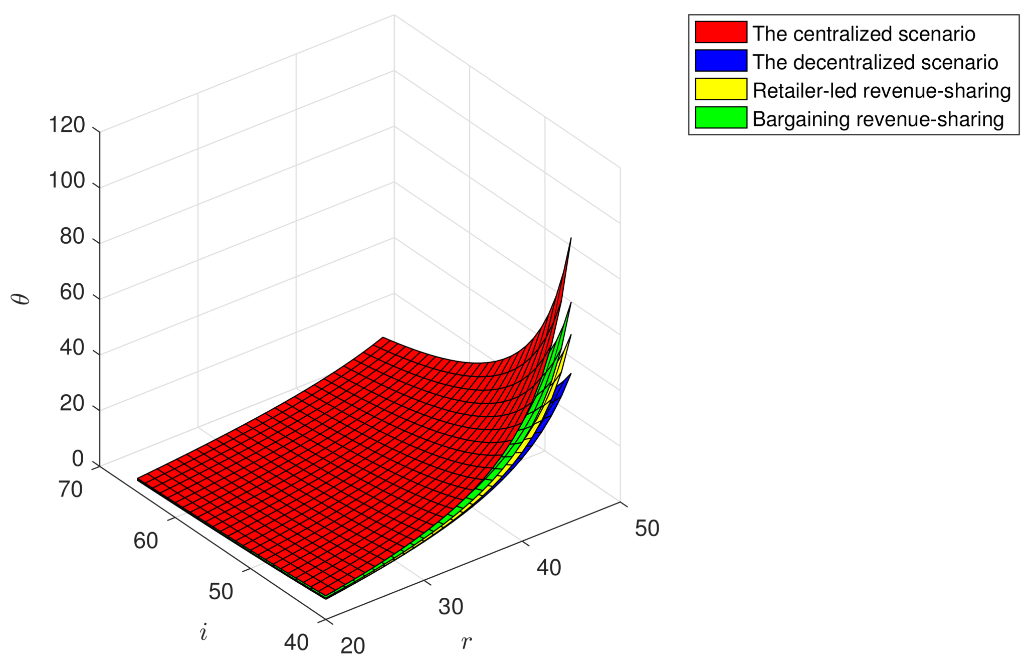
As shown in Figure 2, the green degree ($\theta$) increases with the increase of the customer green sensitivity coefficient (r), and decreases with the increase of the green investment coefficient (i). Correspondingly, when the customer green sensitivity coefficient is at the maximum and green investment coefficient is at the minimum, the green degree reaches the maximum. These indicate that customers’ green sensitivity and preference could promote the improvement of the products’ green level, and the high R&D risks may impede such improvement.

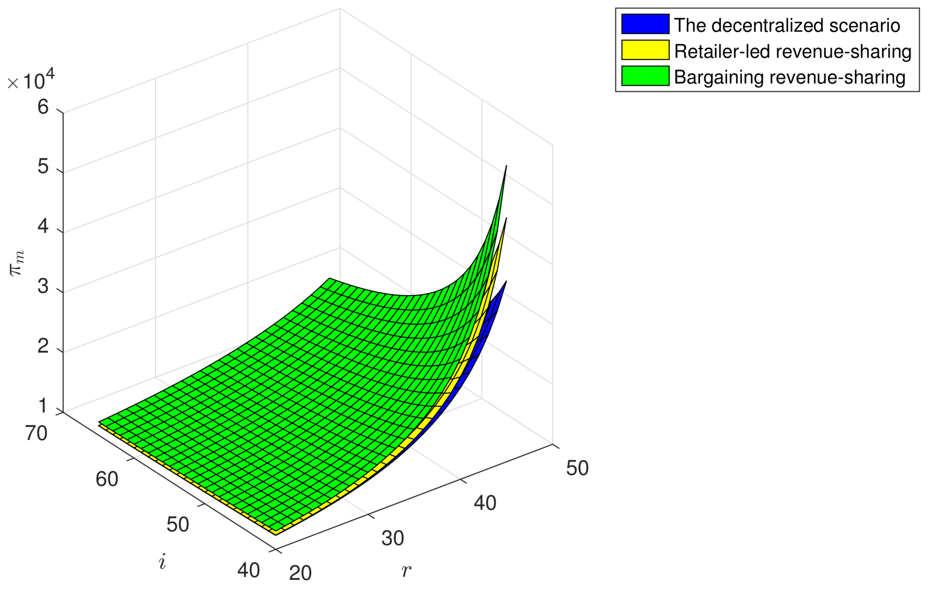
In Figure 3, The manufacturer’s profit (${\pi }_m$) increases with the increase of the customer green sensitivity coefficient (r), and declines with the increase of the green investment coefficient (i). Correspondingly, when the customer green sensitivity coefficient is at the maximum and green investment coefficient is at the minimum, the manufacturer’s profit reaches the maximum. These indicate that customers’ sensitivity and preference to green products could increase the profit of the green manufacturer, and the high R&D cost may reduce the profit.

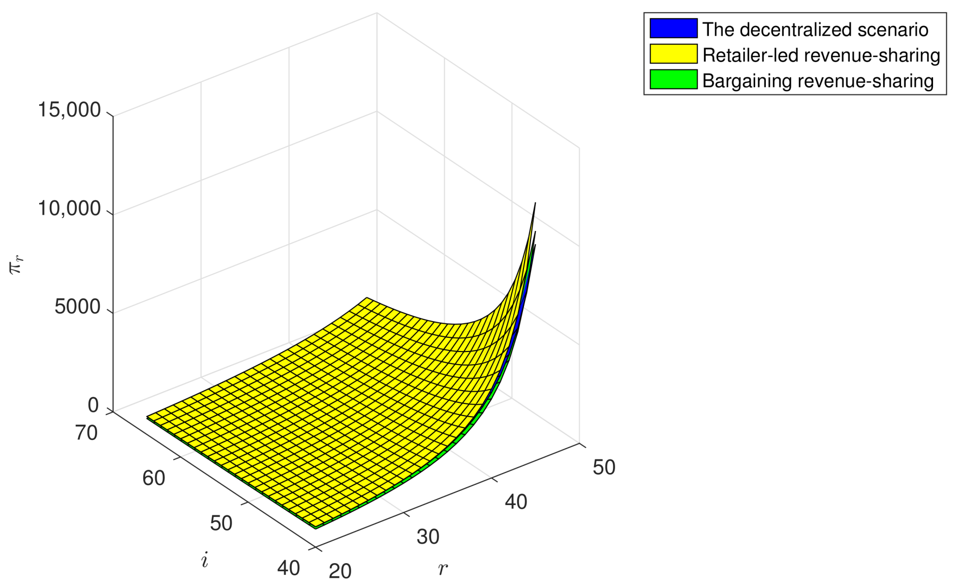
As shown in Figure 4, the retailer’s profit (${\pi }_r$) increases with the increase of the customer green sensitivity coefficient (r), and decreases with the increase of the green investment coefficient (i). Correspondingly, when the customer green sensitivity coefficient is at the maximum and green investment coefficient is at the minimum, the retailer’s profit reaches the maximum. Customer purchasing habits could deeply impact the profit of the retailer. On one hand, customer green consciousness could lead to profit growth. On the other hand, green products R&D may incur higher costs and price, which may drive away price-sensitive customers.

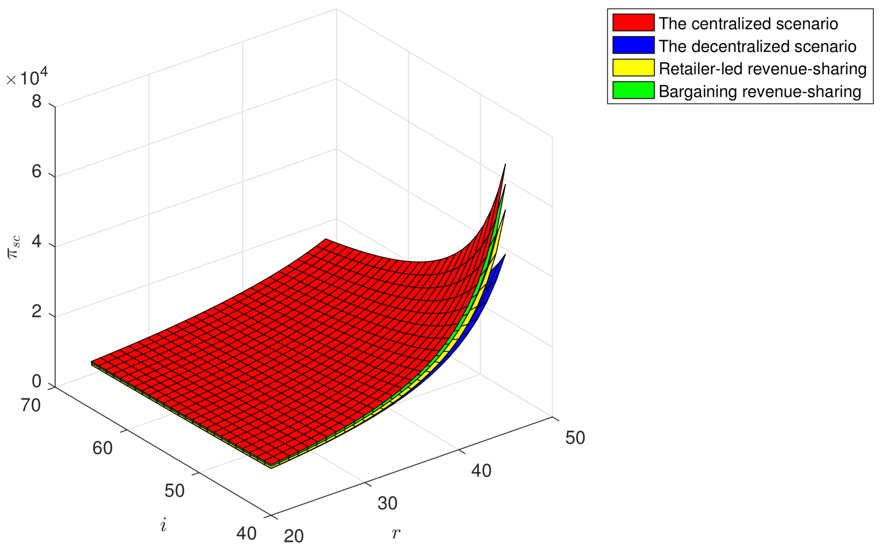
In Figure 5, The overall profit of the GSC (${\pi }_{sc}$) increases with the increase of the customer green sensitivity coefficient (r), and declines with the increase of the green investment coefficient (i). Correspondingly, when the customer green sensitivity coefficient is at the maximum and green investment coefficient is at the minimum, the overall profit of the GSC reaches the maximum. Customer green consciousness could promote the economic performance of the GSC. However, high green products R&D risks may be an impediment.

7. Conclusions

In this paper, we investigate the alignment issues between green level and economic performance of GSC. We are particularly interested to see how the alignment may be achieved through competition and cooperation of the GSC participants. To answer this question, we take into account a dual-distribution GSC composed of a manufacturer, a retailer and customers. Based on this, four game models are established, namely decentralized scenario, centralized scenario, retailer-led revenue-sharing scenario and bargaining revenue-sharing scenario. Moreover, coefficients which represent green product R&D cost, customer green sensitivity and price sensitivity, are introduced into the above models. We compared the optimal decisions of the four game models. We also discussed the impact of green sensitivity and green R&D cost. Main findings are summarized as follows:

(1)

In terms of green degree and profitability, centralized scenario and the two revenue-sharing scenarios are better than decentralized scenario, which indicates that cooperation between the manufacturer and the retailer is more conducive to the GSC’s economic and environmental performance than competition. Given that centralized scenario is difficult to realize due to the high requirement for cooperation level and decision-makers, the two revenue-sharing scenarios are recommended for GSCM practice to achieve the integration of economic and environmental goals.

(2)

Driven by the increase of customer green sensitivity, green degree of product will improve, and profits of the manufacturer, the retailer and the overall GSC will rise. In contrast to customer green sensitivity, high green R&D cost is an obstacle for green innovation and profit growth. Therefore, improving green awareness and reducing green R&D cost will raise green level and profitability of the GSC. Since new technologies always come with additional costs, it is difficult to reduce green R&D cost in reality. Consequently, advocating environmental awareness and promoting green consumption are of vital importance to the GSCM practice.

(3)

In the centralized scenario, the demands in the two channels are equal. In the other three scenarios, the demand in the direct online channel is larger than the demand in the traditional channel. These indicate that the Internet has significantly changed consumption patterns and sale modes, and the online sale has become a major distribution channel of the GSC.

This study has several shortcomings. First, our models assume all of the parameters are certain and deterministic. However, uncertainty widely exists in GSC in reality. Thus, introducing uncertainty into our models for future study is worthwhile. Second, our models use linear demand functions, which have some limitations on simulating the complex activities of GSC. Therefore, establishing non-linear demand functions is the future research direction. Finally, this paper takes customer environmental awareness as a driver promoting the implementation of GSCM. Drivers such as investor focuses, environmental policies and government subsidy may also be important and should be considered in our future study.