Does Poverty Matter in Payment for Ecosystem Services Program? Participation in the New Stage Sloping Land Conversion Program

Abstract

Poverty is increasingly stressed in Payment for Ecosystem Services (PES) schemes, from targeting to outcomes. As the world’s largest PES scheme of its kind, the Sloping Land Conversion Program in China started its new stage (NSLCP), aiming to convert another 2.9 million ha sloping croplands into forest or grasslands. This paper examines whether and to what extent different dimensions of poverty impact households’ participation in the NSLCP. By using the data collected from a key demonstration area, Wuqi County in 2015, based on Sen’s capability theory, we measure the multidimensional poverty of the households, like poverty in education, physical health, food security, rights, assets and living standards. Then, we evaluate the effects of different poverty dimensions on households’ participation in the NSLCP and their efforts to comply with the policy. We find that different dimensions of poverty had very different impacts, as revealed in the participating rate and the intensity of efforts to manage the enrolled lands through different methods. The households with poverty in education, food security, or rights were less likely to be enrolled in the NSLCP. Dimensions like income, health and assets were significant contributions to fulfill the practices required by the NSLCP. Besides, the degree of multidimensional poverty further weakened households’ efforts to manage and protect the trees on enrolled lands.

1. Introduction

The main objective of this study is to evaluate the effects of poverty on participation in Payments for Ecosystem Services (PES) programs to provide policy implications for achieving both conservation and development goals. Why and how to realize the dual goals have been explored for many decades, starting from the discussion on the intricate relationships between poverty, development, and environment conservation [1,2,3], to the studies on the potential effects of PES programs on poverty alleviation [4,5,6,7,8]. Geographically, environmental degradation has always occurred along with poverty issues. Many poor people concentrated in fragile and marginal areas depend intimately on the ecologically-sensitive lands and natural resources [3,9]. They are the primary potential suppliers of ecosystem services (ES) and are supposed to participate in and benefit from the PES programs [4]. This situation suggests that poverty and environmental issues should be addressed together through policy instruments [7], especially in the developing world, where poverty reduction is an essential social goal [4]. Otherwise, the simple targeting policies might easily fall into the poverty-environmental degradation trap [10].

PES schemes are perceived to effectively address both ecological conservation and poverty alleviation. Discussion on whether they could achieve the dual goals in theory and practice has sparked widespread enthusiasm [11,12,13,14]. Practically, governments from many countries (e.g., Brazil, China, Costa Rica, Malawi, and Mexico) implemented large PES programs to reduce both forest degradation and poverty [9,15,16,17]. For example, the Sloping Land Conversion Program (SLCP) in China, the world’s largest PES program of its kind, is one of the crucial measures for China to integrate poverty elimination with environmental conservation. In 2013, the New-Stage Sloping Land Conversion Program (NSLCP) followed up. It is the key phase in which China aims to lift probably another 70 million people from poverty through targeted poverty alleviation and an improvement on the SLCP [18,19]. Many empirical studies also showed that PES programs helped alleviate poverty and improve the wellbeing of the participants through various ways [12,20,21,22,23]. For example, PES programs addressed food security and income increase through in-kind (e.g., grain or seedlings) and cash compensation [20]; facilitated sustainable livelihood through labor reallocation and training courses [21]; promoted the security of land tenure through certificates issuance [22]; and improved the living environment and health risks through improvement in ES and infrastructure [12,23], etc. In all, PES programs can bring not only economic benefits, but also much improvement in other dimensions of wellbeing. That is why we should focus on the ES suppliers in multidimensional poverty.

To fulfill these pro-poor effects of PES programs, it comes to the vital question of the extent to which the poor can equally participate in PES schemes [3,9,24]. Related studies have been conducted a lot, however, they have showed very mixed findings. Some studies have shown that the poorer households were able to participate, even to a greater extent than the better-off households [24] or that economic factors did not determine the participation in PES programs [16,25,26,27]. However, some evidence showed that the poor had more difficulties in participation than the better-off households [28,29]. The potential obstacles for the poor to participate were complex [6,16,29], so were the causes for their poverty state. The poor people described their poverty state by more than just income, but through a wide range of dimensions, like health, social exclusion, low education, bad housing conditions, shame and disempowerment, etc. [30]. In most cases, the deprivation of these wellbeing dimensions worked together for their decisions and behaviors [31,32].

However, the existing studies only told part of the story of how poverty impacts participation in PES programs for two points. (1) Many studies focused on economic dimensions of poverty (income or material assets). Due to the insufficient measurement [30], they could only evaluate poverty’s impacts in a partial way and revealed little about the essential mechanisms of poverty affecting participation [25,26,29,33]. The multidimensional measure of poverty was noted in PES participation [17], but it neglected to further reveal what these dimensions are. (2) Previous studies focused mostly on the first step of the participation process (whether one converted cultivated lands into forests) [8,11,24,26], but the real participation process should include both reforestation and forestland management. The targeted ES and environmental goal will be achieved only if sufficient landowners are enrolled and required management is fulfilled in a sustainable way [12,24].

Therefore, this paper aims to explore the impacts of multidimensional poverty on participation in the NSLCP and enrolled forestlands management. It might contribute to the existing studies from several aspects. (1) Multidimensional poverty presents a novel attribute to study the heterogeneity of potential ES suppliers under the framework of PES. It can explain more about the mechanisms of how different dimensions of poverty affect PES participation theoretically. (2) Going beyond binary participation decisions, the study on land management efforts can implicate pathways to achieve sustainability of ecological outcomes. (3) NSLCP has been improved from the original one. Analysis of participation in the NSLCP calls attention to multiple dimensions of human wellbeing at the beginning of program targeting and implementation. It also provides new evidence and reference for future comparative studies on how policy development affects its targeting outcomes. (4) The empirical results can also implicate which poverty constraints should be addressed for the poor people to participate in PES programs and other policies alike.

The rest of this paper is structured as follows: Section 2 reviews the mechanisms of how poverty impacts participation in PES programs; Section 3 introduces NSLCP, data set, identification of multidimensional poverty, and the empirical approaches; Section 4 analyzes the links between the state of multidimensional poverty and participation, and the empirical results; Section 5 concludes.

2. Mechanisms Linking Multidimensional Poverty with Participation in PES Programs

To reflect multidimensional poverty of the households, we captured whether people were unable to achieve certain minimum thresholds in a variety of dimensions, such as income, education, health, food security, assets, living standard and rights. The selection of dimensions is based on the following consideration: (i) Targets of Millennium Development Goals (MDGs), Sustainable Development Goals (SDGs), and the outline of the Poverty Alleviation Program of Rural China (2011–2020) [34]. (ii) literature on multidimensional poverty and poverty investigations in China [10,30,35,36,37]. (iii) Data avaiable.

Studies on participation in PES scheme can be traced to its early implementation [8,11,24,26]. Factors affecting PES participation were categorized into three aspects: (i) Eligibility (who is selected to participate), (ii) desirability (who is willing to participate), and (iii) ability (who is able to participate) [11]. Thus, we study how different poverty dimensions relate to PES participation from these three aspects.

The first is the relation between poverty and participation eligibility. Eligibility is mainly determined by the targeting criteria and requirements of the PES programs. Gernerally, PES programs targeted geographically the vulnerable ecological areas and set some criteria for land enrollment, like slope, quality, location and tenure, and land use. Many empirical studies showed that land characteristics, rather than economic factors, determined PES participation [6,16,25,26,38]. This land-based targeting in the PES programs was often assumed to favor the poor due to the geographic overlap of poverty concenteration and ecological vulnerability [9,39,40]. For example, in China, 95% of the absolute poverty population were located in key ecological conservation areas [41]. But land tenure required by PES programs might muscle out the poor landholders who suffered right poverty [11,42,43].

Second, the desirability of participation depends much on whether they can gain profits from PES program [33]. The stable payments were more attractive to the economic poor for releasing their short-term liquidity constraints [28,38]. Since the payments were usually fixed in many cases, the desire of participation was mainly determined by the participation costs, including the opportunity costs, transaction costs, etc. The poor with low-productivity lands might have lower opportunity costs for land retirement and a stronger willingness for participation [28,38]. Besides, the risks inherent with land use change or new technology adaptation required by PES programs might also affect households’ willingness to participate. Some studies indicated that many households in food or living poverty might consider more about livelihood stability and prefer a low but stable income over a high but risky one [11,38]. The households with qualified education were assumed to have more environmental concern and to undertake conservation activities [16]. Furthermore, PES was featured as a voluntary mechanism [44], but most government-oriented PES programs were implemented as a centralized approach, like the case of Extrema in Brazil and SLCP in China [6,29,38,45]. Households in right poverty have less autonomy to participate in various public affairs and programs (even though eligible and desirable). Lack of access to information and communication would also lower their enthusiasm and satisfaction towards the programs and harm trust building of governments [16,28].

Third, studies also examined whether the poor who are eligible and desire PES participation are able to do so [16,24]. Multidimensional poverty can fully reflect the constraints for households’ capacity to participate in PES programs. It can be concluded into three aspects: investments to undertake the required practices, technical difficulty, and competitiveness. (i) Due to financial constraint, the households in economic poverty were unable to bear the essential investments and adopt certain land use promoted by the PES program, e.g., forest protection and sustainable management [24,28]. Similarly, due to labor constraints, the households in health poverty could neither supply effective labor for the necessary practices nor find an alternative livelihood. Besides, the poor were excluded from PES programs because of the high transaction costs to negotiate and contract with many small, dispersed landholders [8,24,29]. (ii) Education and technology played crucial roles when required practices were complicated in some sustainable forest management or knowledge-intensive conservation programs [28]. The households in education poverty might find it more difficult to undertake sufficient management without technical assistance, resulting in low survival rate and ecological outcomes. (iii) Competitiveness occurred when the resources or opportunities were limited. The balance of distribution would lean towards the side with strong competitive power. It went beyond the distribution of benefits and costs, touching upon issues of empowerment and autonomy to the households [16]. Households with higher income or more material assets had more inherent abilities and social connections, so they were more powerful in competing for limited access to programs [28,46,47]. Households in right poverty might face many political constraints for PES participation. Neither could they have equal chances to obtain information and to express their opinions in exchange meetings, nor could they have autonomy to follow their choices [16,38].

In short, based on the review of literature above, here come the key hypotheses of this study.

Hypothesis 1 (H1).

Households in education poverty are less likely to participate in PES programs.

Hypothesis 2 (H2).

Health poverty has a negative effect on PES participation and land management.

Hypothesis 3 (H3).

Households in food or living poverty are less likely to participate in PES participation, but they might be more eligible.

Hypothesis 4 (H4).

Right poverty negatively affects PES participation.

Hypothesis 5 (H5).

Economic (asset or income) poverty’s effects are uncertain: positive effect on eligibility and willingness, but negative effect on capacity.

Hypothesis 6 (H6).

The degree of multidimensional poverty has a negative effect on households’ capacity to participate in PES programs and undertake conservation activities.

Although most of the poverty dimensions showed negative effects, households with different poverty dimensions might face different constraints on PES participation and forestland management. In some cases, the eligibility and willingness of the poor would play positive roles in PES participation.

3. Material and Methods

3.1. The NSLCP

As the characteristics of PES programs influence critically how the relationship between poverty and participation plays out, we analyze the process of the SLCP, the changes in the NSLCP, and how these impact the participation of the poor.

The SLCP in China aims to restore ecosystems and to reduce soil erosion and flooding risk. It was designed to encourage the farmers to reforest highly degraded, sloping cultivated lands and afforest barren lands through economic compensation by the central government. It was mainly implemented in ecologically vulnerable and poverty-stricken areas, involving over 124 million rural people [6,9,26,48]. Over its 15 year life (1999–2014), it has achieved reforestation on 9 million ha, afforestation on 20.5 million ha, and an overall annual rate of increase in forest cover of 3% [49]. Then, the NSLCP launched in Yan’an City in 2013, and then expanded nationwide in 2014, aiming to retire all sloping and highly degraded lands (2.8 million ha) by 2020 [49]. Besides, the NSLCP is updated with three primary new features [18], which might affect participation of the poor.

First, the NSLCP adjusted its targeting criteria and priority, which would impact the eligibility of the poor. (i) Slope criteria. In original SLCP, parcels with slopes greater than 25 degrees are targeted in southwest China and parcels over 15 degrees are targeted in the northwest [50]. In the NSLCP, more strict criteria are set for the eligible lands, all the sloping farmlands over 25 degrees are targeted (ca. 1.45 million ha) [49]. (ii) Location criteria. The NSLCP also address the location of eligible sloping farmlands (outside basic farmland redline zone) to guarantee the grain security. The farmlands over 25 degrees but inside the redline zone can only be enrolled after land adjustment work via governments [51]. Enrollment of these lands would cause more difficulties and high transaction costs. As the poor households held more farmlands in poor conditions and less basic farmlands [3,9], they had more eligible lands and cost less to participate in the NSLCP. (iii) Targeting priority. Studies on the original SLCP showed that the program did not target the households by poverty state, despite its auxiliary objective of poverty reduction [6,9]. The NSLCP gives explicit priority to the poor population in poverty concentrated areas, which would help fulfill the pro-poor effects [51].

Second, changes in implementation pattern and autonomy in the NSLCP might improve the state of right poverty and promote the incentive and ability of the poor households to participate. The original SLCP was implemented as a top-to-bottom approach, with tasks distributed from top level to lower level, and the central government played the crucial role in program design and planning [52]. The NSLCP stresses to integrate top-to-bottom and bottom-to-top patterns: Not only giving the local governments more power to design the implementation scheme based on the enrollment applications from the rural households at county level [49], but also giving the households more autonomy to make decisions on participation. For example, in original SLCP, the households had to plant the specified ecological trees (e.g., timber-producing forests) on converted lands, accounting for 80% or more. But in the NSLCP the households can choose the tree species and even develop proper intercropping with dwarf commercial crops on the enrolled lands. It shows full respects for local people’s knowledge and experience of agro-forestry practices, and helps remove some political constraints for the poor to participate and arouse their incentive to manage the converted lands.

Third, the NSLCP also adjusted its focus to support the participating households. (i) Reduction in payments. As one of the biggest concerns of the households, especially for the poor, changes in compensation schemes might impact their willingness to participate. In the NSLCP, the compensating period and total amount are less than those in original SLCP, which might affect households’ incentive. During our survey, lowness of compensation standard was reported as one of the main reasons for landholders’ unwillingness to participate in the NSLCP. (ii) Support for forestry industry. The NSLCP explicitly proposes the supporting measures for the forestry industry to help the participants develop an alternative livelihood [49]. The financial funds from other policies (like Compensation for Forest Ecological Benefits Schemes, Rural Poverty Alleviation Programs, etc.) are pooled together and rearranged for the adjustment of agriculture structure and the development of a featured forestry industry. All these changes indicate that the NSLCP turns to support the participants’ livelihoods through a more sustainable way, going beyond the limited and terminable payments. However, it might lead the program to target households who have the capacity to develop a good production, and muscle out the poor lack of technical skills and education. The stresses on forestland production and management might also be more difficult for the poor with economic and labor constraints.

3.2. Study Area and Data Collection

The survey area, Wuqi County, Yan’an Municipality in northern Shaanxi Province is located in the agro-pastoral transition zone. It is a mountainous area with 70% sloping lands over 25 degrees and 90% highly degraded areas. Prior to the SLCP, it suffered the most severe soil erosion and flooding triggered by extensive farming and open grazing [53]. Wuqi County was the first to launch the SLCP in 1999 and the NSLCP in 2013. It was selected as the demonstration area for subsequent scaling nationwide in China [21,53,54]. Totally, 162,600 ha of sloping cultivated lands were enrolled in the SLCP and a further 14,200 ha in the NSLCP in 2013 and 2014 [55]. We choose Wuqi County as our study site, because it is an epitome area with both ecological sensitivity and poverty concentration, representing other areas targeted by the SLCP. The tremendous changes by the SLCP have attracted lots of studies and surveys conducted here for ecological and environmental issues [21,54,56]. Thus, it was envisaged to provide particularly important information for poverty and participation in the NSLCP.

A pilot survey was conducted during 13 to 16 October 2015 through deep interviews with senior staff from Forest Administration of Wuqi County and sample villages. We obtained the background information about the NSLCP implementation and checked the quality of the questionnaires. Due to the research purpose, we selected the sample villages where NSLCP was implemented. However, based on the pilot field works, we find it difficult to conduct complete random sampling in the study region, as many sample households migrated outside for work (the common situation in rural China) and no appropriate respondents were available to complete the questionnaires with high quality. Therefore, in a formal survey during October and November of 2015, we interviewed the households at home randomly from multiple townships and villages throughout Wuqi County in order to minimize potential location bias in the NSLCP implementation [57]. Finally, the samples covered 300 households from 36 villages in all nine townships of Wuqi County. Due to partial missing responses to the relevant variables, the final sample used for this analysis involved 232 households and the NSLCP participants accounted for 35%.

Furthermore, in order to test the representativeness of the samples, we compared the data with those from the official reports of Wuqi County and previous studies based on random sampling approaches [21,54,58,59,60,61,62], seen in

Table A1. Descriptive statistics of survey data compared with data set from County officials and other studies.

	Sample	County	Province/Implementation Area
1. Demographic characteristics
Family size	3.62 (1.57)	3.96 (1.28)	4.21 (1.35)
Number of labors	2.82 (1.49)	2.45 (1.06)	3.46 (1.37)
Gender of household head: male	0.94 (0.24)	—	0.92
Age of HH. (years)	54.86 (10.83)	55.89 (11.53)	49.78 (11.06)
Age structure: kid ratio(16-)	0.11 (0.16)	—	0.14
Elderly ratio (65+)	0.12 (0.26)	—	0.09
Education of household head:years	6.51 (4.06)	5.92 (3.57)	6.34 (3.58)
2. Socio-economic characteristics
Farmland per capita(ha)	0.16 (0.19)	0.15	0.19 (0.22)
House area (m2)	95.98 (72.05)	—	130.47 (95.94)
House area per capita (m2)	32.87	29.5	34.9
Converted land area(ha)	1.51 (16.78)	2.74 (1.34)	—
Days for farming work	93.22 (145.57)	118.56 (47.67)	—
Days for non-farm work	256.69 (298.25)	231.8 (173.48)	—
Net income per capita	9966	9110	7932

Note: County data was from random sampling in Wuqi County (Li et al., 2015; Zhao et al., 2015) and Statistics Report of Economic and Social Development of Wuqi County in 2012 & 2013; Provincial and implementation area data from stratified random sampling (Kelly and Huo, 2013; Yang and Xu, 2013) and Statistics Report of National Economy and Social Development of Shaanxi in 2013–2014.

. The demographic and socio-economic characteristics from these datasets were similar, which indicated that the study samples were representative.

Questionnaires were designed to collect information about (i) demographic, socio-economic characteristics of households, household livelihood activities and expenditures, income structure, such as agriculture, forestry, out-migration, non-farm activities, etc. (ii) land characteristics of parcels held by the households, slope, soil quality, location, plantation information, land tenure, etc. (iii) Experience with SLCP, participation and subjective perceptions towards the program.

Due to our study purpose, data for measuring households’ poverty state is critical. In order to address reverse causality bias, we tried to measure the poverty state prior to their participating. For example, the net income per capita in 2013 was calculated by the income in 2014 and the changes of the income reported by households (specific questions seen in

Table A2. Key questions and calculations of related variables and indicators.

Variables	Key Questions and Calculations	Literature
1. Dependent variables
Participation	Did you participate in NSLCP: =1 if answer is yes; =0 otherwise
Participation efforts	Time for converted land management (Days): How many did days your family invest labor for enrolled land management last year?
2. Income Poverty variables
Netincome	Annual net income per capita in 2013 = annual net income in 2013/family size; annual net income in 2013 is the sum of net incomes from agriculture, forestry, livestock, outmigration, nonfarm, governmental subsidies in 2014 and income changes compared to last year. (Yuan)	(Statistics Bureau of Shaanxi Province, 2014, 2015)
IPoverty	=1 if net income per capita ≤2600 yuan per year, 0 otherwise
3. Education Poverty variables
EPoverty	=1 if more than half adult members are illiterate or at least one children drop out, 0 otherwise	(Wang and Alkire, 2009; United Nations Development Programme, 2010; Alkire and Santos, 2013; Kolinjivadi et al., 2015)
E1	Education Attainment (E1) presents the general education level of the adults, calculated as a binary variable. E1 = 1 if more than half adult members are illiterate. Respondents were asked about the education level of each family member: 1. Illiterate; 2. Primary school; 3. Middle school; 4. High school; 5. Technical secondary school; 6. College or higher education.
E2	School attendance (E2) presents the schooling status of the children in a household. E2 = 1 if household has at least one school-age child (5–16 in China) is not attending school.
Eduratio	Ratio of family members with education of middle school or higher (%)
4. Health Poverty variables
HPoverty	Ratio of healthy members = number of members in good health/family size (%): Respondents were asked about the health state of each family members: 1. Good; 2. Medium; 3. Bad;	(Ma et al., 2017)
H1	=1 if at least one family member are in bad health. Respondents were asked about the health state of each family member: 1. Good; 2. Medium; 3. Bad.
H2	=1 if a household has at least one mental or physical disability and received the disabled subsidies. Households were asked how much about compensation for disability.
H3	=1 if households’ medical consumption accounts for the largest part compared to other expenditures. Households were asked the detailed expenditures of housing, durable goods, schooling, energy, food, etc. in 2014.
HeadHealth	Health state of household head: 1. Good; 2. Medium; 3. Bad;
5. Food Poverty variables
FPoverty	Value of grain stock per capita = farmland products value/family size (yuan): What is the in-kind value of products on farmlands except those for sales? (yuan)	(Wang and Alkire, 2009) (Xu et al., 2006; Veen and Gebrehiwot, 2011)
F1	=1 if household’s farmland per capita is smaller than the basic line for rural households (0.07 ha).
F2	=1 if household’s consumption for food is less than food demand per capita for balanced nutrition (880 yuan, 400 kg*2.2 yuan/kg). Respondents were asked about household annual cash for food and value of grain stock production. The food demand per capita for balanced nutrition is 400 kg calculated by Chinese Academy of Agricultural Sciences(Chinese Academy of Agricultural Sciences, 1986). And the average price of grain (2.2 yuan/kg) in study region in 2013 comes from documents of Statistics Bureau of Shaanxi Province.
6. Rights Poverty variables
RPoverty	Autonomy scores are calculated as the sum of five binary questions: 1. Did you have autonomy to decide whether to participate or not? 2. Did village ask your opinion about SLCP design and implementation? 3. Did you have autonomy to decide the size to be enrolled? 4. Did you have autonomy to decide which land plot to be enrolled? 5. Did you have autonomy to choose the tree type to plant on converted lands? =1, if the answer is yes; =0 otherwise	(Xu et al., 2010; Wang, 2017)
R1	To reflect households’ engagement in village affairs, households were asked with the question how frequently they attended village meetings and other public affairs for one year: 5-scale from very frequently to seldom. R1 = 1 if the answer is seldom or less.
R2	=1 if autonomy scores equal to 0; =0 otherwise.
R3	Respondents were asked to evaluate the fairness of SLCP implementation: 5-scale from very fair to very unfair. R3 = 1 if the answer is unfair or very unfair, 0 otherwise.
Voluntary	=1 if household has autonomy to decide whether to participate or not, 0 otherwise.
7. Assets Poverty variables
APoverty	Sum of the number of productive assets and durable goods owned, including agricultural machinery or commercial equipment (digging machine, folk lift, etc.), motorized vehicles (bicycle, motorcycle, tractor, and automobile), television, refrigerator, washing machine, and computer.	(Kolinjivadi et al., 2015; Wang, 2017)
A1	=1 if household owns 2 or less durable goods.
Productasset	Sum of the number of assets for production, like vehicles, agricultural machinery or commercial facilities.
8. Living Poverty variables
LPoverty	Living area per capita = house area/family size. (m2) Question: what is the area of your living house? (m2)	(Wang and Alkire, 2009; National Development and Reform Committee, 2016)
L1	Question: Do you own the house you are living? 1. Yes; 0. No; L1 = 1 if the answer is no; L1 = 0 otherwise.
L2	Question: what is the structure of your living house? 1. Wood-mud; 2. Brick-wood; 3. Brick-concrete; 4. Others; L2 = 1 if the house is wood-mud constructed; 0 otherwise.
L3	L3 = 1 if living area per capita is smaller than 25 m2 which is the minimum area for security housing in National 13th Five Planning for Resettlement and Anti-poverty Program.
9. Degree of Multidimensional Poverty
DMP	Degree of multidimensional poverty reflects the number of human wellbeing dimensions deprived. It is the sum of seven binary variables (I, E, H, L, F, A, R) which represent each dimension of poverty.
10. Control Variables
Landslope	Land area with slopes over 25 degrees (ha). Questions were asked about the slope of each land plot held by households: 1. <15 degree; 2. 15–25 degree; 3. 26–35 degree; 4. >35 degree.	(Zbinden and Lee, 2005; Pagiola et al., 2008; Zanella et al., 2014)
Landquality	Ratio of land area with poor soil quality (%). Questions were asked about the soil quality of each land plot held by households: 1.good; 2. medium; 3.bad.
ElderlyR	Ratio of the elderly (%) = the number of elderly(65+)/family size;	(Pagiola et al., 2008; Duesberg et al., 2014; Zanella et al., 2014)
RiskPreference	Risk preference is the sum of the scores of three questions: 1. To what degree would they like to be the first to undertake a new type production. 2. To what degree would they like to undertake the production with higher profit and risk of loss and debt. 3. To what degree do you agree with the idea that only innovative production with and risks can bring wealth to the poor area: 1–5 scores for absolutely unwilling/disagree to absolutely willing/agree.
Payment Gap	Payment gap= (Payments-WTA)/WTA. It presents the deviation of the actual SLCP compensation they got (Payments) from the payments they are willing to accept (WTA). Question was asked about the minimum amount of payments (yuan/ha) the household would like to accept for land conversion.
Remittance	Annual total amount of remittance from outmigration.
Publicity	Publicity presents the transparency of the SLCP implementation in local village. It is sum of three binary questions: 1. did the village have publicity of the distribution of quotas in SLCP? 2. Did the village publicize the compensation process? 3. Did the village publicize the distribution of other tasks for supporting SLCP? =1 if the answer is yes; =0 otherwise.	(Pagiola et al., 2005; Zbinden and Lee, 2005; Uchida et al., 2007; Pagiola et al., 2008; Mullan and Kontoleon, 2012; Duesberg et al., 2014)
Irregularity	Households were asked whether irregular practices existed in local village during SLCP implementation, including illegal logging, enforced conversion, reconversion, delayed payments, etc.
Training	Number of household members ever attend training courses, including training for agro-forestry, husbandry, outmigration, etc.
Accessloan	It presents the development of credit market in local village: Probability for the households to get loans: 5-point scale from impossible to definitely.
Tenure	=1 if the converted lands were issued with certificates; =0 otherwise
Township	Distance from county administrative center:1 = near; 2 = medium; 3 = far	(Bullock and King, 2011)
WillNSLCP	Degree of Willingness to Participate in the NSLCP: respondents were asked the question that whether they are willing to participate in the NSLCP: 5-scale from very unwilling to very willing.
ResponsiMa	Feeling responsible for land management: respondents were asked the question that whether they feel responsible to manage enrolled forestland: 1 = yes, 0 = no.

). The participation-related rights were asked about their autonomy to make decisions when the NSLCP launched. For other poverty dimensions, like education, health, assets, food security and living standards, we only obtained data for 2014. However, we assume it might not cause causality bias, as these dimensions are more stable in the short term than income. As the NSLCP’s impacts on these dimensions are less likely to play out the right away, it might be a little early to evaluate its impacts on participants’ poverty state. However, it is reasonable to evaluate the impacts of poverty state on participation in the NSLCP and participation efforts at the end of 2015.

3.3. Data Analysis

3.3.1. Definition and Measurement of Multidimensional Poverty

The multidimensional view of poverty was derived from Sen and his capability approach [63], where poverty is defined as “deprivation of basic capabilities rather than merely as lowness of income”, including equal access to basic education, health care, employments, social security, etc. However, the widely used measurement, income or consumption-based approach, is not sufficient to capture the state of poverty or all dimensions of social welfare [30,31]. Thus, identification criteria and measurements of poverty are also developed from a unidimensional to multidimensional one [35,64,65]. The human development index (HDI) included health and education dimensions as complementary to income poverty. The multidimensional poverty index (MPI) proposed by Alkire and Foster included three dimensions (health, education, and the standard of living) and 10 indicators. It has been formally publicized in Human Development Report 2010 and adopted in many countries and for different groups (women, children, elderly, etc.) [30,37,66].

Based on previous studies on multidimensional poverty, mechanisms analysis and data available, we included additional vital dimensions (Food security, assets, and rights) here and adopted a tentative set of measurable indicators consistent with a holistic perspective of multidimensional poverty. Here we simplified the measurement of multidimensional poverty and intensity, as we focused more on exploring the impacts of different poverty dimensions, rather than the improvement of identification criteria and methods. Thus, poverty in each dimension was identified by whether the houshold meets the following measurable indicators in

Table 1. Poverty measurements and identification for constructing the degree of multidimensional poverty (DMP).

Dimension	Indicators	Brief Description
I	Income Poverty	I = 1 if Net income per capita is lower than adjusted national poverty line (2600 yuan per year); I = 0 otherwise.
E	Education Poverty	E = 1 if E1 = 1 or E2 = 1; E = 0 otherwise.
	E1: Education attainment	E1 = 1 if half or more adults in household are illiterate (not completing at least one year of schooling)
	E2: School attendance	E2 = 1 if at least one school-age child (5–16 in China) is not attending school
H	Health Poverty	H = 1 if H1 = 1 or H2 = 1 or H3 = 1; H = 0 otherwise.
	H1: Physical health	H1 = 1 if at least one family member is in bad health.
	H2: Disability	H2 = 1 if household has at least one mental or physical disability and received the disabled subsidies.
	H3: Medical consumption	H3 = 1 if household’s medical consumption accounts for the largest part compared to other expenditures (housing, durable goods, schooling, energy, etc.)
L	Living Poverty	L = 1 if L1 = 1 or L2 = 1 or L3 = 1; L = 0 otherwise.
	L1: House ownership	L1 = 1 if household does not own the living house
	L2: House structure	L2 = 1 if the living house is wood-mud constructed
	L3: House area	L3 = 1 if household’s housing area per capita is smaller than the minimum of security housing (25 m2)
F	Food Poverty	F = 1 if F1 = 1 or F2 = 1; F = 0 otherwise.
	F1: Farmland area	F1 = 1 if household’s farmland per capita is smaller than basic line for rural households (0.07 ha).
	F2: Food consumption	F2 = 1 if household’s consumption for food is less than food demand per capita for balanced nutrition.
R	Rights Poverty	R = 1 if R1 = 1 or R2 = 1 or R3 = 1; R = 0 otherwise.
	R1: Public affairs	R1 = 1 if household seldom or less participates in village public affairs
	R2: Autonomy	R2 = 1 if household has no autonomy to participate in NSLCP
	R3: Fairness	R3 = 1 if household thinks SLCP distribution is (very) unfair
A	Assets Poverty	A = 1 if A1 = 1; A = 0 otherwise.
	A1: Physical Assets	A1 = 1 if household owns 2 or less durable goods
	DMP	I + E + H + L + F + R + A, the number of human wellbeing dimensions deprived

Notes: Key questions and calculations are shown in details in Table A2 in Appendix A.

.

Income poverty (I = 1) refers to the level of income unable to satisfy the basic needs of households and is identified by comparing households’ annual net income with the national poverty line determined by the central government. The adjusted poverty line was calculated by the national poverty line set in 2010 (2300 yuan) and CPI indicators of Shaanxi Province [61,67].

However, in the multidimensional context, the identification is more complex and there is no explicit and uniform criteria or poverty line for the poverty dimensions based on human wellbeing. Thus, the selection of indicators and deprivation cutoffs of wellbeing-based poverty are based on relevant studies [10,30,35], the practical contexts and the data available. We scored one point for each dimension of poverty if either of its subindicators meet the condition. For example, education poverty (E) is identified by two indicators: Education attainment (E1) and School attendance (E2). They respectively represent the general education level of the adults and the schooling status of the children in a household. A household is suffering education poverty (E = 1), if half or more adults in the household are illiterate (not completing at least one year of schooling, E1 = 1) or at least one school-age child (5–16 in China) is not attending school (E2 = 1). Similarly, health poverty (H) integrates subjective indicators with objective ones: Physical health (H1), Disability (H2), and Medical consumption (H3). Physical health status is assessed subjectively by respondents and disability and medical consumption can reflect the health condition of the household objectively [36]. Living poverty (L) means a household does not have a stable, safe and basic living space, respectively identified by three indicators: House ownership (L1), House structure (L2), and House area per capita (L3) [36,37,68]. Based on Sen’s poverty theory, food poverty means loss of “the freedom of the individual and the family to establish ownership over an adequate amount of food, which can be done either by growing the food oneself or by buying it in the market” [63]. Thus, it can be measured with food availability and food access [69] and three indicators. Farmland area (F1) reflects the limitation of grain production and food support that significantly determines household food security [70,71]. Food consumption (F2) indicates the access to food production and the food market, measured with grain stock value and cash for food. Right poverty (R) is an important dimension of poverty and is identified by the lack of empowerment to the poor to participate in economic or social activities, or inequitable distribution of resources and benefits [32,38]. The specific rights refer to households’ engagement in village affairs (Public affairs, R1), autonomy in SLCP (Autonomy, R2), and fairness of SLCP implementation (Fairness, R3). Assets Poverty (A) is identified by the deprivation of Physical Assets (A1), with the number of the household’s durable goods limited to two or less. It reflects the state of income aggregation, persistent poverty, and the quality of life [10,32]. We use the number of human wellbeing dimensions deprived to reflect the degree of multidimensional poverty (DMP), calculated as the sum of I, E, H, L, F, R and A, ranging from 0 to 7. How these measurable indicators of each poverty dimension were asked in questionnaires and calculated is completely listed in Table A2.

3.3.2. Estimation Approach

The methodology for this study is based on the previous literature on participation in PES programs. To examine poverty’s impacts on participation (Y), we adopted logit regression models based on the logistic cumulative distribution function, and the probability of participation can be modeled as

$$Prob\left(Y_i=1\right)=\frac{e^{\beta X_i}}{1+e^{\beta X_i}}$$

(1)

where Y_i = 1 if household i participated in the NSLCP and 0 otherwise. $X$ is a set of main explanatory variables reflecting multiple dimensions of poverty and other control variables. Vector $\beta$ is the parameters to be estimated. The logit transformation form of the model is

$$log\left(\frac{Prob\left(Y_i=1\right)}{1-Prob\left(Y_i=1\right)}\right)=\beta X_i$$

(2)

where the effects of $X$ on participation can be estimated by Maximum Likelihood Estimation (MLE). The selection of explanatory variables are presented in Table A2.

Since not all households participated in the NSLCP and not all participating households made efforts in management, the dependent variable, participating efforts (T), is censored at zero. Thus, in order to estimate poverty’s impacts on the time devoted to converted land management, we adopted Tobit models as,

$$T_i^{\ast }={\beta }^{\prime }{X}_i+{\epsilon }_i \epsilon |X~N\left(0,{\sigma }^2\right)$$

(3)

$$T_i=\{\begin{array}{cc}\hfill {\beta }^{\prime }{X}_i+{\epsilon }_i& T_i^{\ast }>0\hfill \\ \hfill 0,& T_i^{\ast }\le 0\hfill \end{array}$$

(4)

where $T_i$ is the time household i invested for converted land management, $T_i^{\ast }$ is a latent variable that satisfies the linear model assumption. $X$ is a set of main explanatory variables reflecting multidimensions of poverty and control variables. $\epsilon$ is an error term that has a normal distribution with mean zero and variance ${\sigma }^2$. Vector ${\beta }^{\prime }$ is the parameters to be estimated by MLE, representing the effects of $X$ on latent variable $T^{\ast }$, and the effects on $T$ can be estimated by

$$E\left(T/X\right)=\Phi \left({\beta }^{\prime }X/\sigma \right) {\beta }^{\prime }X+\sigma \varphi ({\beta }^{\prime }X/\sigma )$$

(5)

where $\mathsf{\Phi }(·)$ is the cumulative distribution and $\varphi (·)$ is density of the standard normal distribution. The marginal effects of a specific variable $x_j$ on T, when other explanatory variables are at mean level, can be estimated by

$$E\left(\frac{\partial E\left(T/X\right)}{\partial x_j}\right)={\beta }_j^{\prime }\Phi \left({\beta }^{\prime }X/\sigma \right)$$

(6)

In all, we set participation and participation efforts as dependent variables (

Table 2. Variables in models and descriptive statistics.

Variables	Brief Description	Mean (SD)	Max	Min
1. Dependent variables
Participation	=1 if household participated in NSLCP, 0 otherwise	0.35 (0.48)	0	1
Participation efforts	Time invested in converted land management (days)	19.19 (29.74)	0	180
2. Main explanatory variables
IPoverty	=1 if net income per capita ≤2600 yuan, 0 otherwise	0.18 (0.39)	0	1
EPoverty	=1 if more than half members illiterate or at least one child drops out, 0 otherwise	0.28 (0.45)	0	1
HPoverty	Ratio of healthy members (%)	0.72 (0.33)	0	1
FPoverty	Value of grain stock per capita (yuan)	629.71 (2049.74)	0	12,500
RPoverty	Autonomy scores (0, 1, 2, 3, 4, 5)	1.76 (1.52)	0	5
APoverty	Number of durable goods owned	4.07 (2.11)	0	14
LPoverty	Living area per capita (m2)	32.87 (35.42)	3.33	150
DMP	Degree of multidimensional poverty	2.92 (1.38)	0	7
3. Control variables
Landslope	Land area with slopes over 25 degrees (ha)	1.24 (1.18)	0	5.33
Landquality	Ratio of land area with poor soil quality (%)	0.29 (0.34)	0	1
WillNSLCP	Degree of Willingness to Participate in the NSLCP	3.75 (1.10)	1	5
ElderlyR	Ratio of the elderly (%)	0.12	0	1
RiskPreference	Risk preference of household (1, 2, 3)	9.53 (3.48)	3	15
Payment Gap	Deviance of payments received from WTA	0.67 (14.73)	−1	4.4
Remittance	Annual total amount of remittance from outmigration	11,326.06 (20181)	0	90,000
Publicity	Publicity of SLCP implementation process(1, 2, 3)	1.34 (1.29)	0	3
Irregularity	Number of irregular practices during SLCP in village	1.20 (1.48)	0	7
Training	Number of household members trained	0.32 (0.69)	0	4
Accessloan	Access to loan: 1 = less, 2 = little … 5 = more	2.03 (1.16)	0	5
Tenure	1 = Converted lands have certificates; 0 otherwise	0.59 (0.49)	0	1
Township	Distance from county administrative center:1 = near; 2 = medium; 3 = far	1.57 (0.81)	1	3

Notes: Key questions and calculations are shown in details in Table A2 in Appendix A. Variables with outliers were winsorized before entering in regression models.

), and seven poverty variable and DMP as the main explanatory variables. Some selected poverty variables were continuous instead of binary poverty variables, in order to avoid the biases from the cutoffs design and to offer a better understanding of poverty’s effects on participation. For example, the ratio of healthy members was used to present the state of health poverty; the value of stock grain per capita was used to reflect the state of food poverty; and living area per capita was directly used as the living condition. Based on theoretical analysis in previous studies, both intra and extra variables were selected as the control variables from three aspects. The details about identification and calculation of these variables can be seen in Table A2.

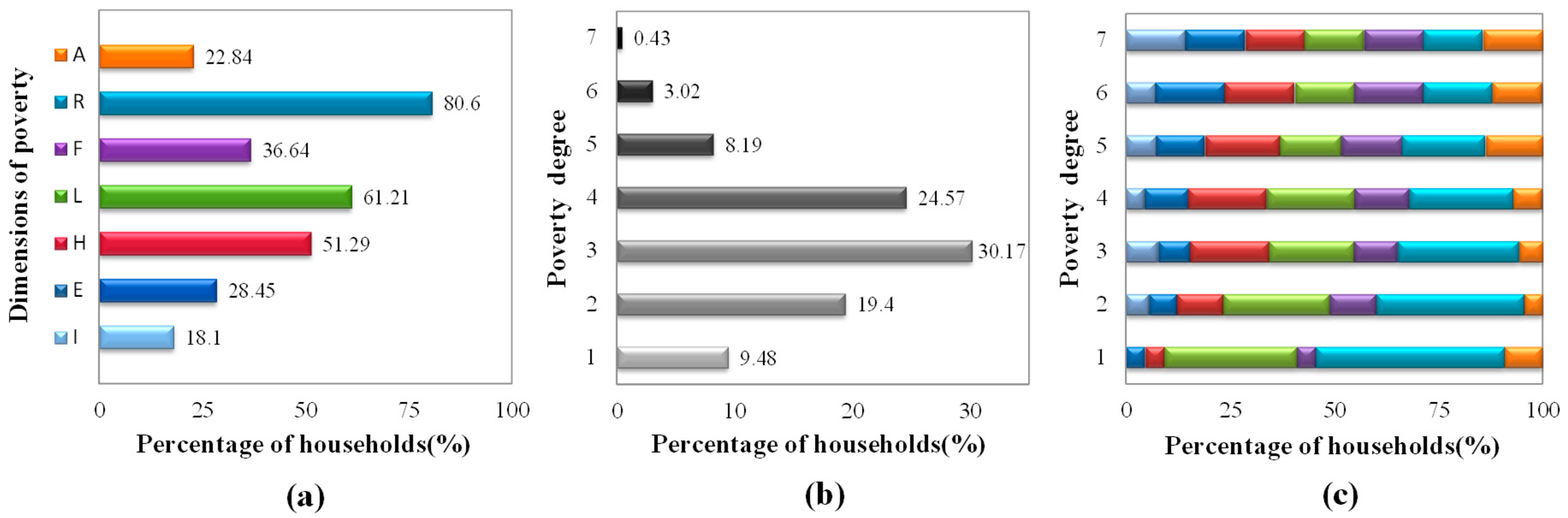
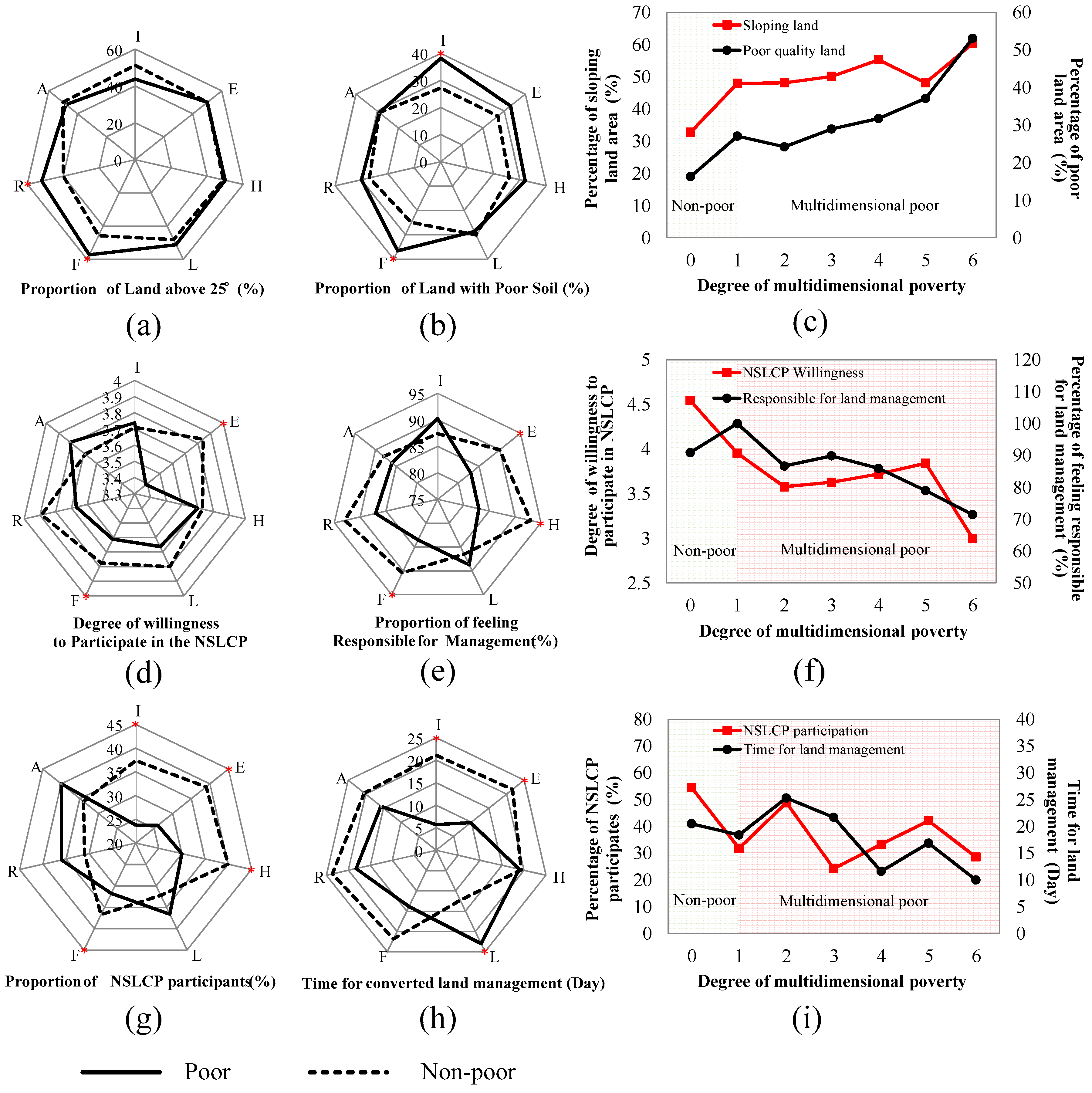
4. Results and Discussion

4.1. Links between Poverty and Participation in the NSLCP

Based on the poverty identification discussed above, the income poverty rate was 18.01% (Figure 1a). However, most of the households experienced multidimensional poverty (85.78%); over half of the households suffered intermediate degrees of multidimensional poverty (three or four dimensions); 30% experienced few dimensions of poverty (one or two dimensions) and 10% experienced severe multidimensional poverty, with five or more aspects of deprivation (Figure 1b).

The most severe poverty dimensions were rights and living condition, with the poor respectively accounting for over 80.60% and 61.21% (Figure 1a). Half of the households fell in poor condition of health and 36.64% suffered food poverty; around a quarter of households had poverty in education and assets. Living and rights poverty also showed the largest shares in every degree of multidimensional poverty (Figure 1c). They both made the main “contribution” to multidimensional poverty; basic public services and improvement in public autonomy and engagement are important and urgent for poverty alleviation and rural development. It just reveals the same fact that the Chinese central government is undergoing a large-scale anti-poverty and development program, aiming to move and resettle the households with poor living conditions in deep mountains to livable areas, to help about 10 million of the poor population to get out of poverty [68].

As participation in the NSLCP depends on a household’s eligibility, desirability and eventually the ability to participate, here we discuss whether and to what extent the poor had the potential to participate in the NSLCP from these three aspects, seen in Figure 2.

Figure 2a,b reflects that the households with less rights, food insecurity, or poorer economic condition had significantly higher percentages of sloping lands and poor soil lands. It indicates that the poor are more eligible for the program and should be given priority to. It also reveals the reason why the NSLCP stressed the priority to poor population in poverty-stricken areas. Moreover, Figure 2c shows the relation between the degree of multidimensional poverty and their land condition. The general trend is that the higher poverty scores the households got, the more fragile and eligible lands they held. It shows the importance to take multiple dimensions of poverty into consideration, as the households with severe multidimensional poverty might hold the most eligible lands for the program.

Households’ participation in the NSLCP also depends heavily on their subjective perceptions towards the program. The households eager for the program accounted for the largest part, 66.38%. But do the poor households have a stronger willingness and motivation to participate in the NSLCP and to manage the converted lands than the non-poor? Not always! Households with different poverty dimensions presented different pictures of self-perception towards the NSLCP. The households with education, health or food poverty had significantly less willingness to participate (Figure 2d) and a lower percentage recognizing their responsibility in management (Figure 2e). Although previous studies showed that households with higher income levels are more desirable to participate in the future SLCP [29], the income dimension had no statistically significant differences in our study. Also, we can see the negative relation between households’ poverty scores and their participation willingness, while not statistically significant (Figure 2f).

The multidimensional poverty can reveal the specific constraints for the eligible and desired poor to participate in the NSLCP and management efforts. Despite volunteerism addressed in the NSLCP enrollment, households’ demands for participation were not fully met by the enrollment design. The data reveals that 61% of households were willing but unable to participate in the NSLCP. It remains to question whether the poor accounted for most of this group. We find that for most poverty dimensions, the poor had a relative lower percentage of participants (Figure 2g) and devoted less time to the NSLCP participation (Figure 2h). Particularly, the households with poverty of income, education, health, and food security might face greater barriers to realize NSLCP participation and its required practices. Also, households with severe multidimensional poverty had a relatively lower participation rate and devoted less time to managing and protecting the converted lands (Figure 2i).

4.2. Poverty’s Impacts on Participation in the NSLCP

Using Stata 12.0, we estimated the effects of different poverty dimensions on participation in the NSLCP by binary logistic regressions. The variance inflation factor (VIF) for the regression coefficients was equal to 3, showing no multi-collinearity among explanatory variables. Also, the correlation matrix presented in

Table A3. Correlation matrix of explanatory variables in regression models.

	IPoverty	DMP	EPoverty	HPoverty	FPoverty	RPoverty	APoverty	LPoverty	EdlerlyR	Landslope
IP.	1.00
DMP	0.18	1.00
EP.	0.06	0.43	1.00
HP.	−0.13	−0.34	−0.29	1.00
FP.	−0.08	−0.24	−0.01	0.13	1.00
RP.	0.09	−0.17	−0.11	0.01	0.15	1.00
AP.	0.02	−0.38	−0.29	0.26	0.13	0.08	1.00
LP.	0.15	−0.34	0.08	−0.08	0.10	0.13	0.10	1.00
Eld.	0.11	0.19	0.31	−0.30	0.01	0.00	−0.10	0.06	1.00
Slo.	−0.11	0.02	−0.03	0.04	0.03	0.01	−0.05	−0.03	0.00	1.00
Qua.	0.12	0.11	0.09	−0.14	−0.14	−0.04	−0.06	0.02	0.08	0.11
Trai.	0.04	−0.13	−0.15	0.06	0.11	0.17	0.10	−0.04	−0.03	−0.02
Loa.	−0.11	−0.15	−0.17	0.11	0.06	0.13	0.12	0.02	−0.07	0.03
Rem	−0.21	−0.04	−0.09	0.15	−0.13	−0.15	0.01	−0.23	−0.21	0.11
Pub.	−0.05	−0.16	−0.04	−0.02	−0.02	−0.09	0.16	0.17	0.01	−0.11
Inrr.	−0.10	0.17	−0.07	−0.12	−0.09	0.07	−0.03	−0.14	0.00	−0.03
Cte.	0.05	−0.10	0.04	−0.10	0.04	0.11	0.01	−0.03	0.05	−0.03
Risk	0.05	0.00	−0.05	0.14	0.10	0.09	0.14	0.01	−0.12	0.05
Gap.	0.02	0.02	−0.05	−0.07	−0.07	0.06	−0.04	0.00	0.06	−0.17
Tp.	0.08	−0.02	−0.05	0.03	0.02	0.27	−0.02	0.01	−0.02	−0.01
	Landquality	Training	Accessloan	Remittance	Publicity	Irregularity	Tenure	Riskprefer.	Payment Gap	Township
IP.
DMP
EP.
HP.
FP.
RP.
AP.
LP.
Eld.
Slo.
Qua.	1.00
Trai.	−0.15	1.00
Loa.	−0.06	0.02	1.00
Rem	0.08	−0.12	0.06	1.00
Pub.	0.03	−0.04	−0.01	−0.01	1.00
Inrr.	0.02	−0.04	−0.04	0.18	−0.01	1.00
Cte.	−0.11	0.00	0.01	−0.05	0.15	−0.06	1.00
Risk	−0.07	0.07	0.11	0.04	−0.16	−0.04	−0.04	1.00
Gap.	0.01	−0.01	−0.03	0.00	0.08	0.04	−0.02	−0.07	1.00
Tp.	0.01	0.01	0.00	−0.03	0.08	−0.03	0.09	0.07	0.06	1.00

shows no statistically significant correlation among explanatory variables. Thus, multi-collinearity is not a problem here.

As discussed above, different poverty dimensions might impact households’ eligibility, desirability and ability to participate in the NSLCP in different ways. Thus, three types of models were built to test the mechanisms how poverty dimensions impact participation: (i) Models without control variables of Landslope and WillNSLCP, (e.g., Models (1), (6), (9)), for evaluating the general effects of poverty on participation; (ii) Models with variables of land eligibility and willingness, for examining the “net” effects of poverty on participation through other mechanisms (e.g., Models (2), (7), (10)); (iii) Models with interaction terms of poverty and Landslope or WillNSLCP, in order to clear how poverty might impact participation through mechanisms of eligibility and desirability (e.g., Models (3–5)).

Regardless of the impacts of eligibility and desire for participation, three out of six poverty dimensions showed statistically significant and negative effects on participation, such as poverty in education, food and rights; however, different poverty dimensions exerted different affecting strengths. Households with poor education experience were less likely to participate in the NSLCP than the non-poor (−0.15 and statistically significant), similar with the findings in PSA participation studies [28]. Those with insufficient food had significantly lower probability to participate in the program. Moreover, the less autonomy the households had, the less likely they could participate in the NSLCP (0.05 and statistically significant).

With the control of eligibility and willingness to participate (Model (2) in

Table 3. Model estimates: marginal effects of multidimensional poverty on participation in the NSLCP.

	Model (1)	Model (2)	Model (3)	Model (4)	Model (5)
	ME (SE)	ME (SE)	ME (SE)	ME (SE)	ME (SE)
EPoverty	−0.15 (0.07) **	−0.14 (0.08) *	−0.15 (0.09) *	−0.14 (0.08) *	−0.14 (0.08) *
HPoverty	−0.17 (0.11)	−0.17 (0.12)	−0.20 (0.11) *	−0.18 (0.11)	−0.17 (0.12)
FPoverty	0.00 (0.00) *	0.00 (0.00) *	0.00 (0.00)	0.00 (0.00)	0.00 (0.00)
RPoverty	0.05 (0.02) *	0.05 (0.02) *	0.05 (0.03) *	0.05 (0.03) **	0.05 (0.02) *
APoverty	−0.03 (0.02)	−0.03 (0.02)	−0.02 (0.02)	−0.02 (0.02)	−0.02 (0.02)
LPoverty	0.00 (0.00)	0.00 (0.00)	0.00 (0.00)	0.00 (0.00)	0.00 (0.00)
ElderlyR	−0.24 (0.15)	−0.25 (0.15)	−0.28 (0.13) **	−0.25 (0.13) *	−0.25 (0.13) *
RiskPreference	−0.01 (0.01)	−0.01 (0.01)	−0.01 (0.01)	−0.01 (0.01)	−0.01 (0.01)
Payment Gap	−0.02 (0.04)	0.00 (0.04)	0.00 (0.05)	−0.00 (0.05)	0.00 (0.05)
Remittance	0.00 (0.00)	0.00 (0.00)	0.00 (0.00)	0.00 (0.00)	0.00 (0.00)
Publicity	0.05 (0.03) **	0.06 (0.03) **	0.06 (0.03) **	0.07 (0.03) **	0.06 (0.03) **
Irregular	−0.04 (0.02)	−0.03 (0.02)	−0.03 (0.02)	−0.04 (0.03)	−0.03 (0.02)
Training	0.05 (0.05)	0.05 (0.05)	0.04 (0.05)	0.04 (0.05)	0.04 (0.05)
Accessloan	−0.02 (0.03)	−0.02 (0.03)	−0.02 (0.03)	−0.02 (0.03)	−0.02 (0.03)
Tenure	0.00 (0.07)	0.00 (0.07)	−0.01 (0.07)	0.01 (0.07)	0.00 (0.07)
Township	0.02 (0.04)	0.03 (0.04)	0.03 (0.04)	0.03 (0.04)	0.03 (0.04)
Landslope	—	0.08 (0.03) **	0.08 (0.03) **	0.08 (0.03) ***	0.08 (0.03) **
Landquality	—	−0.03 (0.10)	−0.02 (0.10)	−0.05 (0.10)	−0.03 (0.10)
WillNSLCP	—	0.00 (0.03)	0.01 (0.03)	0.00 (0.04)	0.00 (0.03)
EPoverty*Landslope	—	—	−0.09 (0.07)	—	—
FPoverty*Landslope	—	—	—	−0.00 (0.00) *	—
RPoverty*Landslope	—	—	—	—	−0.01 (0.02)
Log Likelihood	−137.04	−133.39	−132.59	−131.89	−133.23
Pseudo R2	0.09	0.11	0.12	0.12	0.11

Notes: The table reports marginal effects (ME) and robust/village clustered standard errors (SE in parentheses) from the estimation of Equation (2). Marginal effect presents the participation probability changes caused by independent variables changes, while other variables were held at mean levels. Dependent variable is participation, a binary variable; equals to 1 if household participated in the NSLCP; equals to 0 otherwise. All variables are defined in Table 2 with the detailed description in Table A2. The variables were centered before building the interaction terms. * Significant at 10%; ** significant at 5%; *** significant at 1%.

), the effects of these three dimensions were still statistically significant and without great changes in their strength. It indicates that whether the households with poverty in education, food security and rights can participate in the NSLCP depends much on their capacity rather than eligibility and willingness. Consistent with the hypotheses (H1, H3 and H4), for example, relatively well-educated households usually have more knowledge about how to seek and seize chances for limited access to beneficial programs, while the poor groups might be less competitive to be enrolled, particularly when the requirements are complicated and technical assistance is not available. Those with food insecurity are usually the poorest in the poor and subsistence issues constrain them to bear risks caused by land use changes and to undertake any other conservation activities. Right poverty forms political constraints for the poor households to obtain equal access to the program, especially when the resources are limited or competitive.

Also, the eligible factors showed statistically significant impacts. Households with more sloping lands over 25 degrees had higher probability to be enrolled (0.08 and statistically significant), consistent with policy design and previous studies [25,26]. However, compared with other factors, households’ desire did not have a statistically significant impact on the final enrollment. Similar findings were also drawn from other studies that enrollment distribution was mainly influenced by program administration while willingness of potential participants was less considered during the program implementation [59,72]. Therefore, we introduced the interaction terms of certain poverty dimensions and land slope, to further explore how poverty affects participation though impacts of eligibility. Land slope had negative interaction effects on all three poverty dimensions’ impacts on participation (Models (3–5) in Table 3). Especially for the poor with food insecurity, land slope can explain part of the story how food poverty affects participation. It means although food poverty was an obstacle to participation, land eligibility can relax the constraints for the poor to participate in the NSLCP. These results are consistent with the hypothesis (H3) that eligible criteria of PES programs might favor the poor but the final participation depends a lot on their capacity.

If we only consider the dimension of income (Models (6–8) in

Table 4. Model estimates: marginal effects of income poverty and DMP on participation in the NSLCP.

	Model (6)	Model (7)	Model (8)	Model (9)	Model (10)	Model (11)
	ME (SE)	ME (SE)	ME (SE)	ME (SE)	ME (SE)	ME (SE)
IPoverty	−0.15 (0.08) *	−0.13 (0.08)	−0.14 (0.10)	—	—	—
DMP	—	—	—	−0.02 (0.02)	−0.01 (0.03)	−0.01 (0.03)
ElderlyR	−0.21 (0.12) *	−0.22 (0.13) *	−0.22 (0.13) *	−0.21 (0.12) *	−0.22 (0.13) *	−0.21 (0.13)
RiskPreference	−0.01 (0.01)	−0.01 (0.01)	−0.01 (0.01)	−0.01 (0.01)	−0.01 (0.01)	−0.01 (0.01)
Payment Gap	0.00 (0.04)	0.01 (0.04)	0.01 (0.04)	−0.01 (0.04)	0.01 (0.04)	0.01 (0.04)
Publicity	0.04 (0.02)	0.05 (0.03)	0.05 (0.03) *	0.04 (0.03)	0.05 (0.03) *	0.05 (0.03) *
Irregular	−0.02 (0.02)	−0.02 (0.02)	−0.02 (0.02)	−0.02 (0.02)	−0.02 (0.02)	−0.02 (0.02)
Training	0.07 (0.04)	0.07 (0.05)	0.07 (0.05)	0.07 (0.05)	0.06 (0.05)	0.06 (0.05)
Accessloan	−0.01 (0.03)	−0.01 (0.03)	−0.01 (0.03)	−0.01 (0.03)	−0.01 (0.03)	−0.00 (0.03)
Tenure	0.03 (0.07)	0.03 (0.07)	0.04 (0.07)	0.02 (0.07)	0.03 (0.07)	0.02 (0.07)
Township	0.06 (0.04)	0.06 (0.04)	0.06 (0.04)	0.05 (0.04)	0.06 (0.04)	0.06 (0.04)
Landslope	—	0.07 (0.03) **	0.07 (0.03) **	—	0.08 (0.03) **	0.07 (0.03) **
Landquality	—	−0.01 (0.10)	−0.02 (0.10)	—	−0.03 (0.10)	−0.04 (0.10)
WillNSLCP	—	0.02 (0.03)	0.02 (0.03)	—	0.02 (0.03)	0.02 (0.03)
IPoverty*Landslope	—	—	−0.03 (0.09)	—	—	—
DMP*Landslope	—	—	—	—	—	0.04 (0.02) *
Log Likelihood	−142.43	−138.62	−138.57	−143.83	−139.63	−138.14
Pseudo R2	0.05	0.08	0.08	0.04	0.07	0.08

Notes for Table 4 were omitted here, the same with those for Table 3.

), we find that income poverty had significant negative impacts on participation in the NSLCP. However, the mechanisms might be more complicated, as hypothesized (H5). With the control of the land slope and willingness, the negative effects weakened and turned insignificant. Despite the potential correlations between income poverty and land condition, the interaction effects in Model (8) were not statistically significant. It indicates that it was the land characteristics that determined participation in the NSLCP, rather than economic factors, consistent with previous studies on original SLCP [6,26]. Consistent with the hypothesis (H6), the degree of multidimensional poverty also had negative effects (not statistically significant) on participation in all models (Models (9–11) in Table 4).

Besides, all participation models show the statistically significant effects of policy publicity. A transparent program process facilitated participation, while irregular practices during the program process played a negative role. This is in line with the studies stressing the importance of access to sufficient and effective information [27,28,29].

We further provide robustness tests concerning the cutoffs and selection of poverty variables. For example, to examine whether Epoverty captures the poverty state of education, as well as the possible non-linearity of its impacts, we included the education ratio (Eduratio) and its square term in the regressions for Equation (2) (

Table A4. Robustness tests of the econometric models.

NSLCP	Participation		Participation Efforts
	Original	Robust	Original	Robust	Original	Robust
EPoverty → Eduratio	−0.14 (0.08) *	0.61 (0.37) *	−2.96 (3.58)	−4.68 (3.74)	——	——
Eduratio square	——	−0.64 (0.39)	——	——	——	——
HPoverty → headhealth	−0.17 (0.12)	−0.14 (0.12)	9.05 (5.11) *	−5.43 (2.21) **	——	——
FPoverty → Self-sufficient ratio	0.00 (0.00) *	0.05 (0.09)	0.00 (0.00)	0.00 (0.00)	——	——
RPoverty → voluntary	0.05 (0.02) *	0.13 (0.07) *	−1.67 (1.38)	−1.50 (1.29)	——	——
APoverty → Productasset	−0.03 (0.02)	−0.03 (0.02)	3.25 (1.57) **	6.82 (2.99) **	——	——
LPoverty	0.00 (0.00)	0.00 (0.00)	−0.11 (0.08)	−0.15 (0.08) *	——	——
IPoverty → netincomeper	——	——	——	——	−12.88 (6.19) **	0.00 (0.00) **
Income square	——	——	——	——		0.00 (0.00) **
ElderlyR	−0.25 (0.15)	−0.27 (0.14) *	3.03 (10.07)	5.93 (10.90)	−2.25 (10.96)	−0.10 (13.09)
RiskPreference	−0.01 (0.01)	−0.01 (0.02)	−0.80 (0.55)	−0.73 (0.52)	−0.12 (0.50)	−0.03 (0.61)
Payment Gap	0.00 (0.04)	0.00 (0.07)	1.24 (2.30)	1.97 (2.23)	−0.40 (1.95)	−0.03 (2.31)
Remittance	0.00 (0.00)	0.00 (0.05)	−0.00 (0.00)	0.00 (0.00) *	——	——
Publicity	0.06 (0.03) **	0.06 (0.03) **	1.62 (1.54)	2.35 (1.39) *	2.20 (1.25) *	2.70 (1.64)
Irregular	−0.03 (0.02)	−0.02 (0.00)	1.92 (1.68)	1.88 (1.64)	0.37 (1.68)	0.20 (1.38)
Training	0.05 (0.05)	0.08 (0.03) *	0.41 (1.83)	0.89 (1.69)	1.46 (1.68)	1.51 (2.17)
Accessloan	−0.02 (0.03)	−0.01 (0.10)	3.45 (1.78) *	2.24 (1.52)	2.34 (1.62)	2.45 (1.79)
Tenure	0.00 (0.07)	0.01 (0.03)	7.01 (3.72) *	6.95 (3.59) *	5.55 (3.67)	6.51 (4.11)
Township	0.03 (0.04)	0.04 (0.01)	1.18 (2.23)	0.93 (2.32)	0.03 (1.77)	−0.75 (2.40)
Landslope	0.08 (0.03) **	0.08 (0.04) **	5.44 (1.89) ***	6.13 (1.98) ***	4.18 (1.76) **	3.57 (1.61) **
Landquality	−0.03 (0.10)	−0.04 (0.03)	−6.73 (4.86)	−6.74 (5.14)	−8.42 (5.09) *	−10.13 (5.91) *
WillNSLCP	0.00 (0.03)	0.01 (0.04)	0.14 (1.96)	0.25 (2.35)	−1.02 (2.41)	−1.16 (1.95)
Log Likelihood	−133.39	−130.99	−295.71	−290.05	−302.23	−300.76
Pseudo R2	0.11	0.10	0.05	0.05	0.03	0.03

Notes: The table reports marginal effects (ME) and robust/village clustered standard errors (SE in parentheses) from the estimation of Equations (2) and (6). Dependent variables are respectively participation (whether participated in NSLCP) and participation efforts (time devoted to converted land management). Revised represents the models in revised manuscript; Robust represents the models for robustness tests with key poverty variables replaced with proxies. All variables are defined in Table 2 with detailed description in Table A2. * Significant at 10%; ** significant at 5%; *** significant at 1%.

). We find that the coefficients on education poverty remain essentially unchanged and had significantly negative impacts in both regressions. Its square term was not statistically significant, which means families with the lowest education level are least likely to participate in NSLCP.

4.3. Poverty’s Impacts on Participation Efforts

The efforts to fulfill the forestland management to keep the trees alive are much more crucial to the outcomes and sustainability of the programs. However, nearly a quarter of NSLCP participants only converted their lands but did not undertake management.

Table 5. Model estimates: marginal effects of multidimensional poverty on participation efforts.

	Model (12)	Model (13)	Model (14)	Model (15)	Model (16)	Model (17)
	ME (SE)	ME (SE)	ME (SE)	ME (SE)	ME (SE)	ME (SE)
EPoverty	−3.24 (4.15)	−2.96 (3.58)	−2.84 (3.59)	−3.18 (5.07)	−3.65 (3.66)	−3.16 (5.09)
HPoverty	9.85 (5.09) *	9.05 (5.11) *	9.37 (5.20) *	7.55 (6.36)	8.52 (5.11) *	6.27 (6.46)
FPoverty	0.00 (0.00)	0.00 (0.00)	0.00 (0.00)	0.00 (0.00)	0.00 (0.00)	0.000.00)
RPoverty	−1.27 (1.34)	−1.67 (1.38)	−1.60 (1.35)	−2.05 (1.52)	−1.74 (1.39)	−1.74 (1.50)
APoverty	2.82 (1.72)	3.25 (1.57) **	3.18 (1.54) **	2.96 (1.01) ***	2.90 (1.50) *	3.35 (1.00) ***
LPoverty	−0.07 (0.08)	−0.11 (0.08)	−0.12 (0.08)	−0.11 (0.08)	−0.10 (0.08)	−0.06 (0.08)
ElderlyR	0.95 (10.46)	3.03 (10.07)	2.35 (10.17)	3.63 (11.33)	2.35 (10.08)	0.52 (11.72)
RiskPreference	−0.50 (0.55)	−0.80 (0.55)	−0.79 (0.55)	−0.74 (0.58)	−0.82 (0.55)	−1.16 (0.62) *
Payment Gap	0.50 (2.44)	1.24 (2.30)	1.40 (2.27)	1.69 (2.18)	0.97 (2.28)	1.78 (2.20)
Remittance	−0.00 (0.00)	−0.00 (0.00)	−0.00 (0.00) **	−0.00 (0.00) **	−0.00 (0.00) **	−0.00 (0.00) *
Publicity	0.35 (1.50)	1.62 (1.54)	1.55 (1.53)	1.54 (1.61)	1.47 (1.57)	1.67 (1.61)
Irregular	1.84 (1.86)	1.92 (1.68)	1.87 (1.66)	1.89 (1.50)	1.96 (1.66)	1.97 (1.50)
Training	0.92 (1.70)	0.41 (1.83)	0.08 (1.97)	0.22 (2.01)	0.26 (1.80)	1.39 (2.08)
Accessloan	3.19 (1.83) *	3.45 (1.78) *	3.54 (1.79) **	3.35 (1.64) **	3.58 (1.79) **	2.84 (1.67) *
Tenure	6.09 (3.82)	7.01 (3.72) *	6.70 (3.58) *	7.28 (4.02) *	7.09 (3.71) *	5.79 (4.03)
Township	0.89 (2.14)	1.18 (2.23)	0.88 (2.19)	1.01 (2.34)	1.29 (2.22)	1.15 (2.35)
Landslope	—	5.44 (1.89) ***	5.13 (1.91) ***	5.92 (1.50) ***	5.54 (1.85) ***	4.54 (1.55) ***
Landquality	—	−6.73 (4.86)	−5.94 (4.90)	−5.27 (5.45)	−6.86 (4.90)	−5.72 (5.41)
WillNSLCP	—	0.14 (1.96)	0.23 (1.96)	1.12 (1.97)	−0.12 (2.02)	0.44 (1.92)
HPoverty*Landslope	—	—	3.80 (6.21)	—	—	—
APoverty*Landslope	—	—	—	1.34 (0.71) *	—	—
HPoverty*WillNSLCP	—	—	—	—	−7.55 (4.27)*	—
APoverty*WillNSLCP	—	—	—	—	—	−1.84 (0.95) *
Log Likelihood	−302.08	−295.71	−295.52	−294.02	−294.67	−293.92
Pseudo R2	0.03	0.05	0.05	0.06	0.05	0.06

Notes: The table reports marginal effects (ME) and robust/village clustered standard errors (SE in parentheses) from the estimation of Equation (6). Marginal effects present changes of time for converted lands management caused by independent variables changes, while other variables were held at mean levels. Dependent variable is participation efforts, a censored variable, the time invested for converted land management. All variables are defined in Table 2 and described in details in Table A2. * significant at 10%; ** significant at 5%; *** significant at 1%.

and

Table 6. Model estimates: marginal effects of income poverty and DMP on participation efforts.

	Model (18)	Model (19)	Model (20)	Model (21)	Model (22)	Model (23)	Model (24)	Model (25)
	ME (SE)	ME (SE)	ME (SE)	ME (SE)	ME (SE)	ME (SE)	ME (SE)	ME (SE)
IPoverty	−15.16 (6.73) **	−12.88 (6.19) **	−12.52 (5.99) **	−14.79 (8.00) *	—	—	—	—
DMP	—	—	—	—	−1.94 (0.99) *	−1.91 (0.98) *	−1.56 (0.93) *	−1.24 (0.92)
ElderlyR	−5.55 (10.98)	−2.25 (10.96)	−2.04 (10.91)	−2.54 (11.03)	−4.92 (10.03)	−1.83 (10.21)	6.06 (11.79)	−1.78 (10.00)
RiskPreference	0.03 (0.53)	−0.12 (0.50)	−0.10 (0.51)	−0.16 (0.51)	0.14 (0.53)	−0.07 (0.49)	0.08 (0.49)	0.03 (0.49)
Payment Gap	−0.70 (1.97)	−0.40 (1.95)	−0.43 (1.97)	−0.44 (1.95)	−0.58 (2.17)	−0.24 (2.11)	−0.10 (2.13)	−0.64 (2.26)
Publicity	1.15 (1.21)	2.20 (1.25) *	2.27 (1.26) *	2.28 (1.21) *	1.16 (1.15)	2.11 (1.21) *	1.80 (1.20)	1.88 (1.24)
Irregular	0.76 (1.63)	0.37 (1.68)	0.38 (1.67)	0.28 (1.70)	1.57 (1.66)	0.98 (1.68)	0.98 (1.66)	0.79 (1.68)
Training	1.77 (1.67)	1.46 (1.68)	1.41 (1.65)	1.37 (1.62)	1.53 (1.51)	1.29 (1.52)	1.37 (1.53)	1.10 (1.48)
Accessloan	2.23 (1.61)	2.34 (1.62)	2.45 (1.65)	2.23 (1.59)	2.32 (1.51)	2.54 (1.56)	1.80 (1.58)	2.50 (1.51) *
Tenure	4.60 (3.70)	5.55 (3.67)	5.81 (3.79)	5.13 (3.73)	4.65 (3.68)	5.64 (3.67)	5.86 (3.67)	5.19 (3.69)
Township	0.06 (1.66)	0.03 (1.77)	−0.08 (1.72)	−0.14 (1.74)	−0.29 (1.63)	−0.16 (1.78)	−0.16 (1.82)	0.19 (1.80)
Landslope	—	4.18 (1.76) **	4.04 (1.78) **	4.17 (1.73) **	—	4.53 (1.72) ***	4.39 (1.75) **	4.59 (1.73) **
Landquality	—	−8.42 (5.09) *	−8.27 (5.07)	−8.78 (1.73) *	—	−7.83 (5.11)	−7.08 (5.07)	−8.10 (5.16)
WillNSLCP	—	−1.02 (2.41)	−1.04 (2.40)	−0.48 (2.71)	—	−1.76 (2.49)	−1.61 (2.52)	−2.27 (2.62)
IPoverty*Landslope	—	—	−1.98 (4.73)	—	—	—	—	—
IPoverty*WillNSLCP	—	—	—	3.86 (9.35)	—	—	—	—
DMP*Landslope	—	—	—	—	—	—	−1.15 (0.81)	—
DMP*WillNSLCP	—	—	—	—	—	—		−1.49 (0.87) *
Log Likelihood	−306.16	−302.23	−302.15	−302.15	−307.75	−303.13	−302.52	−302.52
Pseudo R2	0.02	0.03	0.03	0.03	0.01	0.03	0.03	0.03

Notes for Table 6 were omitted here, the same with those for Table 5.

show how poverty dimensions impact efforts to convert land management.

Models (12–17) in Table 5 presents different impacts of poverty dimensions on the time devoted to land management. Amongst these, health poverty played the most important role. Good physical health had positive impacts on participation efforts (9.85 and statistically significant). It still had a statistically significant influence (9.05) when controlling the effects of land condition and willingness variables (Model (13)). It indicates that the households in health poverty cannot fulfill management due to some other mechanisms. They had more difficulties and higher costs for access to effective labor force, which constrains their management investment in the PES program, consistent with the hypothesis (H2).

As shown in Model (12), the general effects of assets poverty were not statistically significant, but with the control of land and willingness effects (Model (13)), it showed significant negative effects on participation efforts. The poor with fewer durable goods devoted significantly less time to enrolled land management in the NSLCP (3.25). Assets here can represent wealth state of the households and the main elements for land-based production. The changes of poverty’s effects in these two models indicate that land condition and willingness of participation can explain part of poverty’s impacts on converted land management.

How does health poverty and asset poverty affect participation efforts through land condition and willingness of participating in the NSLCP? Interaction effects in Models (14–17) show that both willingness and land slope influenced the impacts of poverty on management, but had very different effects. Households’ desire for participating in the NSLCP can weaken the negative effects of health poverty and asset poverty on converted land management (−7.55 and statistically significant). For example, the households in poor physical health conditions with a desire for NSLCP were more likely to undertake management than those enrolled by force. On the other hand, poor land conditions, like sloping land, would exacerbate these constraints. For example, the households in asset poverty with more sloping land were more likely to avoid their duty of management.

The income-poor’s efforts to manage converted land were significantly less than the non-poor in Models (18–21) in Table 6. They devoted less time to converted land management, no matter whether the land condition and willingness were controlled or not. The interaction effects in Models (20–21) were not statistically significant. It indicates that the negative effects on management were not attributed to the poor condition of their lands or their unwillingness towards the program. The financial constraints might be the greatest obstacle for poor participants to undertake the required management. The variable Accessloan also told the same fact that if the credit market worked well for the poor households, it would be more accessible for them to obtain more funds to support conservation and management.

Not only did the single poverty dimensions, like health poverty, asset poverty and income poverty have a statistically significant influence on households’ efforts with participation, but so too did the degree of multidimensional poverty have important and negative effects (−1.94 and statistically significant). With the multidimensional poverty deepening, households’ investment for managing the converted lands decreased. The interaction effects of households’ willingness were statistically significant to alleviate these negative effects (−1.49). It indicates that households’ positive perceptions towards the program would promote more incentive to manage the enrolled lands.

Besides, the converted land tenure meant a lot in management decisions. The households issued with certificates of converted lands were likely to devote more energy to manage and protect the trees.

We also provide robustness tests for participation efforts models concerning the cutoffs and selection of poverty variables. For example, to examine whether Ipoverty captures the poverty state of the economic dimension, as well as its possible non-linear effects, we include net income per capita and its square term in the regressions for Equation (6) (Table A4). We find that the coefficients on income poverty remained essentially unchanged and had significant negative effects in both regressions. Its square term was also statistically significant, but the turning point was very high at nearly the top 5% of net income. It means that for most households in poor rural areas, the income poverty always played negative effects on participation efforts in the NSLCP.

5. Conclusions and Implications

This study has empirically studied the impacts of multidimensional poverty on households’ participation in the NSLCP, and their efforts to manage the enrolled forestlands. Based on the survey data collected in a typical NSLCP area, we measured multidimensional poverty of the households and explored how different poverty dimensions affect their participating in the NSLCP and the time devoted to land management through eligibility, desire and ability. Although many studies focused on income poverty and its impacts, our study showed that most households in marginal rural areas suffered in more than one poverty dimension and that low living standards and rights poverty are the main contributors to multidimensional poverty. Our study also contributes to the literature on poverty and participation. Some studies showed that income or assets poverty did not determine participation in PES programs. However, our study showed that poverty in other non-economic dimensions had crucial roles in NSLCP enrollment and could explain more about the potential and constraints of the poor to undertake required conservation practices.

Most poverty dimensions had negative effects on participation, and it is interesting to find how different dimensions alter households’ eligibility, desire, and ability to participate in the NSLCP in different ways during different stages of the program’s process. During the process of conversion and reforestation, land eligibility was the key for enrollment to achieve the efficiency and validity of the program, which was assumed to provide opportunities for the poor with marginal lands [9,39,40]. However, our study showed that the income poor were not given priority to participate in the NSLCP, and poverty in education, food security, and rights formed the main constraints for the poor to participate; however, the eligibility of the poor can help relax these constraints on participation.

During the stage of follow-up management and maintenance, income, asset and health poverty formed the main investment constraints for the poor to undertake required practices. Both financial capital and effective labor were the significant contributors to fulfill the management of converted lands. The more severe multidimensional poverty they suffered, the more various constraints they would face, and the less efforts they could make to manage converted land. Thus, to achieve expected outcomes and sustainability of the program, many supports are needed to alleviate the constraints caused by multidimensional poverty.

This study also brings some valuable policy implications for improving targeting effects and sustainable implementation of the PES programs alike. First, multiple dimensions of poverty should be comprehensively considered in the enrollment process to achieve effective pro-poor targeting and consequentially, to validate outcomes. Incentive mechanisms should be developed to overcome the obstacles for the poor to participate. For example, for the multidimensional poor, collective contracting might be a good choice through which the eligible sloping lands held by the individual poor can be enrolled and managed collectively in the PES program. It can also reduce transaction costs and interest the program implementers [28]. At the same time, more attention should be paid to willingness and perspectives of potential participants during policy design and implementation to cultivate incentive towards the policies and required duties. However, our study showed that households’ subjective perceptions towards the program did not determine their final participation and political barriers for the poor’s participation still existed. The autonomy of the households should be realized rather than just be rhetoric. In short, the PES might have targeted the poorest areas but not the poorest people there, as there might be various constraints for the poor people with multidimensional poverty to participate in the program. Thus, supporting measures, like training courses and credits should be addressed and followed up to enhance their welfare of different dimensions and to remove the barriers for households to undertake and sustain conservation practices.

Our study also has certain limitations that can be reconciled in future research. First, as NSLCP is a newly-launched program, we only focus on poverty’s impacts on participation, but the effects of the program on multidimensional wellbeing were only assumed based on previous studies. Future studies can proceed to explore the effects of PES programs on poverty alleviation in multiple dimensions, like education, health, income, etc. Second, our data were collected at household level, and even the information related to village status were reported by the households. Further studies can associate with multi-level data from structured interviews with both households and village leaders, so that more external factors can be directly controlled. Finally, longitudinal data could be followed to study and compare the poverty’s effects on participation over time. Environmental conservation and poverty alleviation are increasingly heralded as joint objectives through policy instruments, especially in the developing world. Our findings suggested promise for PES in a context where poverty and conservation were stressed together; however, economic, social, political, and many other constraints remained for the poor to participate and benefit.

References

1. Reardon, T.; Vosti, S.A. Links between rural poverty and the environment in developing-countries—Asset categories and investment poverty. World Dev. 1995, 23, 1495–1506. [Google Scholar] [CrossRef]
2. Narain, U.; Gupta, S.; Veld, K.V. Poverty and the environment: Exploring the relationship between household incomes, private assets, and natural assets. Land Econ. 2008, 84, 148–167. [Google Scholar] [CrossRef]
3. Barbier, E.B. Poverty, development, and environment. Environ. Dev. Econ. 2010, 15, 635–660. [Google Scholar] [CrossRef]
4. Milder, J.C.; Scherr, S.J.; Bracer, C. Trends and future potential of payment for ecosystem services to alleviate rural poverty in developing countries. Ecol. Soc. 2010, 15, 4. [Google Scholar] [CrossRef]
5. Bulte, E.H.; Lipper, L.; Stringer, R.; Zilberman, D. Payments for ecosystem services and poverty reduction: Concepts, issues, and empirical perspectives. Environ. Dev. Econ. 2008, 13, 245–254. [Google Scholar] [CrossRef]
6. Démurger, S.; Pelletier, A. Volunteer and satisfied? Rural households’ participation in a payments for environmental services programme in Inner Mongolia. Ecol. Econ. 2015, 116, 25–33. [Google Scholar] [CrossRef]
7. Rodríguez, L.C.; Pascual, U.; Muradian, R.; Pazmino, N.; Whitten, S. Towards a unified scheme for environmental and social protection: Learning from PES and CCT experiences in developing countries. Ecol. Econ. 2011, 70, 2163–2174. [Google Scholar] [CrossRef]
8. Grieg-Gran, M.; Porras, I.; Wunder, S. How can market mechanisms for forest environmental services help the poor? Preliminary lessons from Latin America. World Dev. 2005, 33, 1511–1527. [Google Scholar] [CrossRef]
9. Gauvin, C.; Uchida, E.; Rozelle, S.; Xu, J.; Zhan, J. Cost-effectiveness of payments for ecosystem services with dual goals of environment and poverty alleviation. Environ. Manag. 2010, 45, 488–501. [Google Scholar] [CrossRef] [PubMed]
10. Kolinjivadi, V.; Grant, A.; Adamowski, J.; Kosoy, N. Juggling multiple dimensions in a complex socio-ecosystem: The issue of targeting in payments for ecosystem services. Geoforum 2015, 58, 1–13. [Google Scholar] [CrossRef]
11. Pagiola, S.; Arcenas, A.; Platais, G. Can payments for environmental services help reduce poverty? An exploration of the issues and the evidence to date from Latin America. World Dev. 2005, 33, 237–253. [Google Scholar] [CrossRef]
12. Ferraro, P.J.; Hanauer, M.M.; Miteva, D.A.; Nelson, J.L.; Pattanayak, S.K.; Nolte, C.; Sims, K.R. Estimating the impacts of conservation on ecosystem services and poverty by integrating modeling and evaluation. Proc. Natl. Acad. Sci. USA 2015, 112, 7420–7425. [Google Scholar] [CrossRef] [PubMed] [Green Version]
13. Fisher, J.A.; Patenaude, G.; Giri, K.; Lewis, K.; Meir, P.; Pinho, P.; Rounsevell, M.D.A.; Williams, M. Understanding the relationships between ecosystem services and poverty alleviation: A conceptual framework. Ecosyst. Serv. 2014, 7, 34–45. [Google Scholar] [CrossRef]
14. Antle, J.M.; Stoorvogel, J.J. Payments for ecosystem services, poverty and sustainability: The case of agricultural soil carbon sequestration. Nat. Res. Manag. Policy 2009, 31, 133–161. [Google Scholar]
15. Mazunda, J.; Shively, G. Measuring the forest and income impacts of forest user group participation under Malawi’s Forest Co-management Program. Ecol. Econ. 2015, 119, 262–273. [Google Scholar] [CrossRef]
16. Zanella, M.A.; Schleyer, C.; Speelman, S. Why do farmers join Payments for Ecosystem Services (PES) schemes? An assessment of PES water scheme participation in Brazil. Ecol. Econ. 2014, 105, 166–176. [Google Scholar] [CrossRef]
17. Pagiola, S. Payments for environmental services in Costa Rica. Ecol. Econ. 2008, 65, 712–724. [Google Scholar] [CrossRef] [Green Version]
18. National Development and Reform Commission. Notice of Issuing New-Stage SLoping Land Conversion Program Scheme; National Development and Reform Commission: Beijing, China, 2014.
19. China State Council. Accurate Targeting of Poverty Alleviation Program; China State Council: Beijing, China, 2015.
20. Duan, W.; Lang, Z.; Wen, Y. The effects of the sloping land conversion program on poverty alleviation in the Wuling mountainous area of China. Small Scale For. 2015, 14, 331–350. [Google Scholar] [CrossRef]
21. Li, H.; Yao, S.; Yin, R.; Liu, G. Assessing the decadal impact of China’s sloping land conversion program on household income under enrollment and earning differentiation. For. Policy Econ. 2015, 61, 95–103. [Google Scholar] [CrossRef]
22. Liu, Z.; Gong, Y.; Kontoleon, A. How do payments for environmental services affect land tenure? Theory and evidence from China. Ecol. Econ. 2018, 144, 195–213. [Google Scholar] [CrossRef]
23. Ferraro, P.J.; Hanauer, M.M. Protecting ecosystems and alleviating poverty with parks and reserves: ‘Win-Win’ or tradeoffs? Environ. Resour. Econ. 2010, 48, 269–286. [Google Scholar] [CrossRef]
24. Pagiola, S.; Rios, A.R.; Arcenas, A. Can the poor participate in payments for environmental services? Lessons from the Silvopastoral Project in Nicaragua. Environ. Dev. Econ. 2008, 13, 299–325. [Google Scholar] [CrossRef]
25. Feng, L.; Xu, J. Farmers’ willingness to participate in the next-stage grain-for-green project in the three gorges reservoir area, China. Environ. Manag. 2015, 56, 505–518. [Google Scholar] [CrossRef] [PubMed]
26. Uchida, E.; Xu, J.; Xu, Z.; Rozelle, S. Are the poor benefiting from China’s land conservation program? Environ. Dev. Econ. 2007, 12, 593–620. [Google Scholar] [CrossRef]
27. Duesberg, S.; Upton, V.; O’Connor, D.; Dhubháin, Á.N. Factors influencing Irish farmers’ afforestation intention. For. Policy Econ. 2014, 39, 13–20. [Google Scholar] [CrossRef]
28. Zbinden, S.; Lee, D.R. Paying for environmental services: An analysis of participation in costa Rica’s PSA program. World Dev. 2005, 33, 255–272. [Google Scholar] [CrossRef]
29. Mullan, K.; Kontoleon, A. Participation in payments for ecosystem services programs: Accounting for participant heterogeneity. J. Environ. Econ. Policy 2012, 1, 235–254. [Google Scholar] [CrossRef]
30. Alkire, S.; Santos, M.E. A multidimensional approach: Poverty measurement & beyond. Soc. Indic. Res. 2013, 12, 239–257. [Google Scholar]
31. Andam, K.S.; Ferraro, P.J.; Sims, K.R.; Healy, A.; Holland, M.B. Protected areas reduced poverty in Costa Rica and Thailand. Proc. Natl. Acad. Sci. USA 2010, 107, 9996–10001. [Google Scholar] [CrossRef] [PubMed] [Green Version]
32. Wang, X. The Measurement of Poverty Theories and Methods, 2nd ed.; Social Sciences Academic Press: Beijing, China, 2017. [Google Scholar]
33. Guo, H.; Li, B.; Hou, Y.; Lu, S.; Nan, B. Rural households’ willingness to participate in the grain for green program again: A case study of Zhungeer, China. For. Policy Econ. 2014, 44, 42–49. [Google Scholar] [CrossRef]
34. China State Council. Outline of Poverty Alleviation Program of Rural China; China State Council: Beijing, China, 2011.
35. Alkire, S. Foster, J. Counting and multidimensional poverty measurement. J. Public Econ. 2011, 95, 476–487. [Google Scholar] [CrossRef]
36. Ma, B.; Ding, H.; Wen, Y. Impacts of biodiversity on multi-dimensional poverty. J. Agrotech. 2017, 4, 116–128. [Google Scholar]
37. Wang, X.; Alkire, S. Mesurement of multi-dimensional poverty in China: Estimation and policy implication. Chin. Rural. Econ. 2009, 4, 10–23. [Google Scholar]
38. Xu, J.T.; Tao, R.; Xu, Z.G.; Bennett, M.T. China’s sloping land conversion program: Does expansion equal success? Land Econ. 2010, 86, 219–244. [Google Scholar] [CrossRef]
39. Zilberman, D.; Lipper, L.; McCarthy, N. When could payments for environmental services benefit the poor? Environ. Dev. Econ. 2008, 13, 255–278. [Google Scholar] [CrossRef]
40. Alix-Garcia, J.; De Janvry, A.; Sadoulet, E. The role of deforestation risk and calibrated compensation in designing payments for environmental services. Environ. Dev. Econ. 2008, 13, 375–394. [Google Scholar] [CrossRef]
41. Ministry of Environmental Protection. Plan for Conserving National Ecologically Vulnerable Zones; China’s Ministry of Environmental Protection: Beijing, China, 2008.
42. Wunder, S. Payments for Environmental Services: Some Nuts and Bolts; CIFOR Occasional Paper No 42; Center for International Forestry Research: Jakarta, Indonesia, 2005. [Google Scholar]
43. Bremer, L.L.; Farley, K.A.; Lopez-Carr, D. What factors influence participation in payment for ecosystem services programs? An evaluation of Ecuador’s SocioPáramo program. Land Use Policy 2014, 36, 122–133. [Google Scholar] [CrossRef]
44. Wunder, S. Payments for environmental services and the poor: Concepts and preliminary evidence. Environ. Dev. Econ. 2008, 13. [Google Scholar] [CrossRef]
45. Bennett, M.T. China’s sloping land conversion program: Institutional innovation or business as usual? Ecol. Econ. 2008, 65, 699–711. [Google Scholar] [CrossRef]
46. Pagiola, S.; Zhang, W.; Colom, A. Can payments for watershed services help finance biodiversity conservation? A spatial analysis of Highland Guatemala. J. Nat. Resour. Policy Res. 2010, 2, 7–24. [Google Scholar] [CrossRef] [Green Version]
47. Landell-Mills, N.; Porras, I.T. Silver Bullet or Fools’ Gold? A Global Review of Markets for Forest Environmental Services and Their Impacton the Poor; Food and Agriculture Organization of the United Nations: Rome, Italy, 2002. [Google Scholar]
48. Li, X.; Zuo, T.; Jin, L. Environment and Poverty: The Chinese Practice and International Experiences; Social Sciences Academic Press: Beijing, China, 2005. [Google Scholar]
49. State Forestry Administration. New-stage Sloping Land Conversion Program Plan (2014–2020); State Forestry Administration: Beijing, China, 2014.
50. Uchida, E.; Xu, J.T.; Rozelle, S. Grain for green: Cost-effectiveness and sustainability of China’s conservation set-aside program. Land Econ. 2005, 81, 247–264. [Google Scholar] [CrossRef]
51. State Ministery of Finance. Notice of Enlarging the Scale of New-stage Sloping Land Conversion Program; State Ministery of Finance: Beijing, China, 2015.
52. China State Council. Regulation for SLCP; China State Council: Beijing, China, 2002.
53. Yao, S.; Li, H. Agricultural productivity changes induced by the sloping land conversion program: An analysis of Wuqi county in the Loess Plateau region. Environ. Manag. 2010, 45, 541–550. [Google Scholar] [CrossRef] [PubMed]
54. Zhao, M.J.; Yin, R.S.; Yao, L.Y.; Xu, T. Assessing the impact of China’s sloping land conversion program on household production efficiency under spatial heterogeneity and output diversification. China Agric. Econ. Rev. 2015, 7, 221–239. [Google Scholar] [CrossRef]
55. SLCP Administration Office. Statistics of Annual Scales of SLCP in Counties of Yan’an City; SLCP Administration Office: Yan’an, China, 2015. [Google Scholar]
56. Lin, Y.; Yao, S. Impact of the sloping land conversion program on rural household income: An integrated estimation. Land Use Policy 2014, 40, 56–63. [Google Scholar] [CrossRef]
57. Bullock, A.; King, B. Evaluating China’s slope land conversion program as sustainable management in Tianquan and Wuqi Counties. J. Environ. Manag. 2011, 92, 1916–1922. [Google Scholar] [CrossRef] [PubMed]
58. Statistics Burea of Wuqi County. Statistics Report of Economic and Social Development of Wuqi County; Statistics Burea of Wuqi County: Wuqi, China, 2012.
59. Kelly, P.; Huo, X. Do farmers or governments make better land conservation choices? Evidence from China’s Sloping Land Conversion Program. J. For. Econ. 2013, 19, 32–60. [Google Scholar] [CrossRef]
60. Yang, X.; Xu, J. Program sustainability and the determinants of farmers’ self-predicted post-program land use decisions: Evidence from the sloping land conversion program in China. Environ. Dev. Econ. 2013, 19, 30–47. [Google Scholar] [CrossRef]
61. Statistics Burea of Shaanxi Province. Statistics Report of National Economy and Social Development of Shaanxi; Statistics Burea of Shaanxi Province: Xi’an, China, 2014.
62. Statistics Burea of Shaanxi Province. Statistics Report of National Economy and Social Development of Shaanxi; Statistics Burea of Shaanxi Province: Xi’an, China, 2013.
63. Sen, A. Development as Freedom; Oxford University Press: Oxford, UK, 1999. [Google Scholar]
64. Bourguignon, F.; Chakravarty, S.R. The measurement of multidimensional poverty. J. Econ. Inequal. 2003, 1, 25–49. [Google Scholar] [CrossRef]
65. Atkinson, A.B. Multidimensional deprivation: Contrasting social welfare and counting approaches. J. Econ. Inequal. 2003, 1, 51–65. [Google Scholar] [CrossRef]
66. United Nations Development Programme. The Real Wealth of Nations: Pathways to Human Development; Human Development Report 2010; United Nations Development Programme: New York, NY, USA, 2010. [Google Scholar]
67. Statistics Burea of Shaanxi Province. Rural Households’ Income Increase Bring Great Poverty Reduction in Shaanxi Poor Areas; Statistics Burea of Shaanxi Province: Xi’an, China, 2015.
68. National Development and Reform Commission. National 13th Five Planning for Resettlement and Anti-poverty Program; National Development and Reform Commission: Beijing, China, 2016.
69. Food and Agriculture Organization. The State of Food Insecurity in the World 2014; FAO: Rome, Italy, 2015. [Google Scholar]
70. Veen, A.; Gebrehiwot, T. Effect of policy interventions on food security in Tigray, Northern Ethiopia. Ecol. Soc. 2011, 16. [Google Scholar] [CrossRef]
71. Xu, Z.; Xu, J.; Deng, X.; Huang, J.; Uchida, E.; Rozelle, S. Grain for green versus grain: Conflict between food security and conservation set-aside in China. World Dev. 2006, 34, 130–148. [Google Scholar] [CrossRef]
72. He, J.; Sikor, T. Notions of justice in payments for ecosystem services: Insights from China’s Sloping Land Conversion Program in Yunnan Province. Land Use Policy 2015, 43, 207–216. [Google Scholar] [CrossRef]
Figure 1. State of multidimensional poverty. Three graphs respectively show the percentages of households with different poverty dimensions (a), households with different degrees of multidimensional poverty (b), seven dimensions in each level of multidimensional poverty (c). Only 4.74% households did not have any dimension of poverty (not shown in the figure).
Sustainability 10 01888 g001
Figure 2. Links between poverty and participation in the NSLCP. Radar Charts present the differences between the poor and non-poor, identified by multiple poverty dimensions in eligibility (a,b), desirability (d,e) and ability (g,h). The red asterisks indicate the differences are statistically significant. Line charts study the differences in eligibility (c), desirability (f) and ability (i) among groups with different DMP.
Sustainability 10 01888 g002