Carbon Dioxide (CO₂) Emission Reduction Potential in East and South Coastal China: Scenario Analysis Based on STIRPAT

Abstract

East and south coastal China is made up of a cluster of six developed provinces whose CO₂ emissions account for one third of the total CO₂ emissions in China. As such, it is meaningful to predict carbon emissions in this region to assess whether China can achieve emission reduction targets. This paper employed STIRPAT to analyze the factors impacting the carbon emissions of this area from 2000 to 2015, including population (POP), urbanization (UR), GDP per capita (GDP), energy intensity (EI), and industrial structure (IS). The results showed that GDP was mainly responsible for increasing carbon emissions while EI played a significant role in reducing it. Considering the importance of GDP, EI, and IS obtained from regression analysis, basic, highest-rate, middle, and advanced scenarios were set to predict carbon emissions according to different change rates. In the basic scenario, carbon intensity was reduced by 48.5% in 2020 compared to 2005, which was slightly higher than the national target of 40–45%, and was reduced by 59.7% in 2030, which was close to a 60–65% reduction. Nevertheless, in the advanced scenario, carbon intensity was reduced by 51.7% in 2020 and 69.1% in 2030 compared to 2005, which were higher than the national targets. Therefore, improving energy efficiency, optimizing energy structure, and adjusting industrial structure were suggested to be major strategies for carbon intensity mitigation.

1. Introduction

The world economy is developing rapidly, and China’s enormous role cannot be ignored. At present, China has become the second-largest economy worldwide. However, economic growth is always accompanied by a large amount of energy consumption, especially fossil fuels consumption. It is clear that Chinese carbon emissions are closely linked to the consumption of fossil fuels, which makes China the world’s largest carbon emitter, accounting for 23.4% of carbon emissions in the world [1,2]. Consequently, mitigation of the greenhouse effect has become an urgent issue in China. Several targets have been set by the government for conserving energy and reducing emissions. In December 2009, a CO₂ reduction target of 40–45% by 2020, compared to 2005 levels, was set by the government [3]. In the “13th Five-Year Plan” (2016–2020), the government put forward specific indicators of National Economic and Social Development, in which energy efficiency and carbon intensity were proposed to be reduced by 15% and 18% in 2020 respectively, compared to 2016. In addition, in 2015, the Chinese government promised that carbon emissions would not rise no later than 2030, and carbon intensity would be reduced by 60–65% compared to 2005 [4].

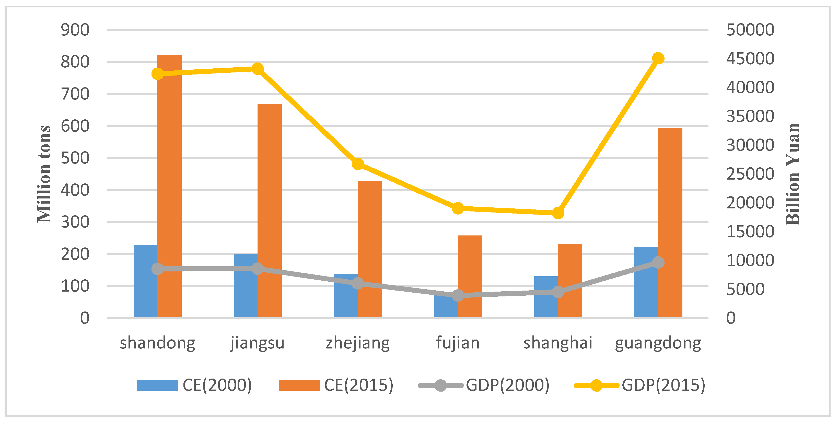
East and south coastal China, including Shandong, Zhejiang, Jiangsu, Shanghai, Fujian, and Guangdong (hereinafter referred to as “the Region” according to the research in Reference [5]), is a cluster of the country’s most economically developed provinces. The Region contains the Yangtze River Delta, including Zhejiang, Jiangsu, Shanghai [6], and the Pearl River Delta, including most areas of Guangdong [7]. Because of its location along the coast, import and export trade promotes the growth of the regional GDP [8]. In 2015, the Region’s GDP was 217610.8 BY, accounting for more than one half of the country’s total GDP. It was not only the first region to implement the reform and opening up policies, but also served as an experimental base for important national plans [5]. Although the Region accounts for only a small portion of the country’s land, its population was 406.5 million and carbon emissions were 3252.2 Mt in 2015, which accounted for approximately one third of the national total [9]. Therefore, the Region is extremely vital for estimating whether the country can achieve emission reduction targets.

For all that, there is little research on the Region for in-depth study. In this paper, six provinces in east and south coastal China were taken into consideration for analysis. We used the STIRPAT model to study the factors impacting carbon emissions. For the sake of developing a better understanding of the current state of development, this paper explored the Environmental Kuznets Curve (EKC) relationship of per capita GDP/urbanization and carbon emissions in the Region. In addition, according to the “13th Five-Year Plan”, four different scenarios were set up to predict the Region’s contribution to the national 2020 and 2030 emission reduction targets. In the light of the scenario analysis, this paper proposed several corresponding effective policy suggestions. In conclusion, this study was conducted to resolve following issues: firstly, to analyze the factors influencing carbon emissions, further verifying the existence of the EKC relationship; secondly, to predict the Region’s contribution to the national emission reduction targets; and thirdly, to put forward related policy recommendations.

The rest of this paper is structured as follows. Section 2 provides the literature review. Section 3 introduces the methodology and data sources. Section 4 reports the results and discussions. Section 5 gives the conclusions and policy implications.

2. Literature Review

For the choice of the research object, different studies have different emphases. Some studies selected diverse industries as research objects. Zhang et al. [10] studied the factors impacting CO₂ emissions in the transportation sector. They found that the traffic activity effect was the main factor increasing energy consumption, while adjusting energy intensity effects could effectively reduce it. Wang et al. [4] studied carbon emissions in high, mid, and low energy consumption sectors from 1996 to 2012, setting three scenarios to estimate whether 2020 and 2030 carbon emission targets could be reached, and corresponding policy recommendations were given to the sub-sectors. Meng et al. [11] researched the relationship between CO₂ emissions and its influencing factors in the power industry from 2001 to 2013. They concluded that the government should optimize the industrial export structure and raise the awareness of household electricity saving to alleviate the carbon dioxide emissions of the electricity industry in the future. In addition, some studies selected different areas as research objects. For example, some studies concentrated on national carbon emissions (e.g., [12,13]). Wang et al. [14] and Wang and Zhao [15] studied the differences in the impact factors on carbon emissions in eastern, central, and western China. Song et al. [6] and Yu et al. [7] selected the Yangtze River Delta and the Pearl River Delta as the object of study, respectively. In detail, Song et al. [6] used the LMDI model to analyze the driving effects of economic scale, population size, energy intensity, and energy structure on carbon emissions in the Yangtze River Delta. The implementation of targeted carbon reduction measures was found to help greatly reduce the national carbon emissions. Meanwhile, to a certain extent, the research method was also applicable to other specific regions in China. Yu et al. [7] studied the impact of traffic control policies on O₃ emissions in the Pearl River Delta. The results of this study provided some basic information to help understand the impact of control policies on ambient O₃ in highly developed areas in China. In addition, some studies selected a single province as the object of study. Wang et al. [16] conducted an econometric model to investigate carbons emission in Guangdong Province from 1980–2010. Xu et al. [17] used the input-output relationship of the SDA model to discuss carbon emissions in Jiangsu. At present, only Gao et al. [5] chose the Region as the research object, using the LMDI model to analyze the influencing factors of carbon emissions from 2000–2012.

Various methods were used by the existing studies on the impact factors of carbon emissions, among which logarithmic mean Divisia index (LMDI) and STIRPAT are two of the most commonly applied due to their strong applicability. Wang et al. [4], Xu et al. [18], and Yan et al. [19] examined the affecting factors of national greenhouse gas emissions using the LMDI model. Guo et al. [20], Liu et al. [21], and Xin [22] employed the LMDI model and the research objects they selected were Shanghai, Jiangsu, and Beijing, respectively. They all decomposed factors into the following categories: carbon emission coefficient, energy structure, energy efficiency, industry share, GDP. Liu et al. [23], Lin and Long [24], and Xie et al. [25] applied LMDI and focused on the carbon emission indexes of different industries, including industrial, chemical, and petroleum coking industries, which decomposed factors into CO₂ emission coefficient, industry share, energy efficiency, average output, and industry size. However, the number of impact factors that the LMDI model can consider is limited, so this method does not allow multivariate analysis [16]. The STIRPAT model, however, has fewer constraints on the selection factors than LMDI. Zhang and Tan [12] employed the STIRPAT model to study the demographic factors influencing China’s carbon emissions, and these factors included adult illiteracy rate, higher education proportion, population intensity, population share, and the like. Salahuddin et al. [26] used the STIRPAT model to analyze the impact factors of Internet use on carbon emissions in Organization for Economic Cooperation and Development (OECD) countries, and creatively selected the number of Internet users per 100 people as a technical factor. Tan et al. [27] applied the STIRPAT model to predict the carbon emissions of 2020 and 2030 in Chongqing, in which the energy structure, industrial structure, and technological advancement were chosen to replace the technical factors (T) in the model. Compared to LMDI, the STIRPAT model has a wider range of factors selection, so the results are more comprehensive and convincing [16].

Additionally, the EKC hypothesis for income and pollution can be traced back to the pioneering work of Grossman and Krueger [28], who reported that pollution index and GDP had an inverted U-shaped relation. It is worth noting that the EKC has significant merits. Its inverted U-shape reflects that economic growth can promote environmental improvement. The prerequisite for this result is to implement effective environmental policies while raising the economic level [29]. EKC has been widely used to estimate the current stage of development in the region. York et al. [30] found that STIRPAT can accurately represent the functional form of the relation between emissions and economic growth. After that, a number of studies used STIRPAT to study the EKC relationship between GDP and carbon emissions. Diao et al. [31] verified the EKC hypothesis concerning the economic level and carbon emissions of Zhejiang. Later, the research direction was related to the trend of urbanization and carbon emission, and further confirmed the development level of the researched region. Ouyang and Lin [32] employed the STIRPAT model to compare the impact of urbanization on CO₂ emissions in China and Japan. He et al. [33] found the inverted U-shape curve relation between urbanization and carbon emissions in different development level regions. Zhao et al. 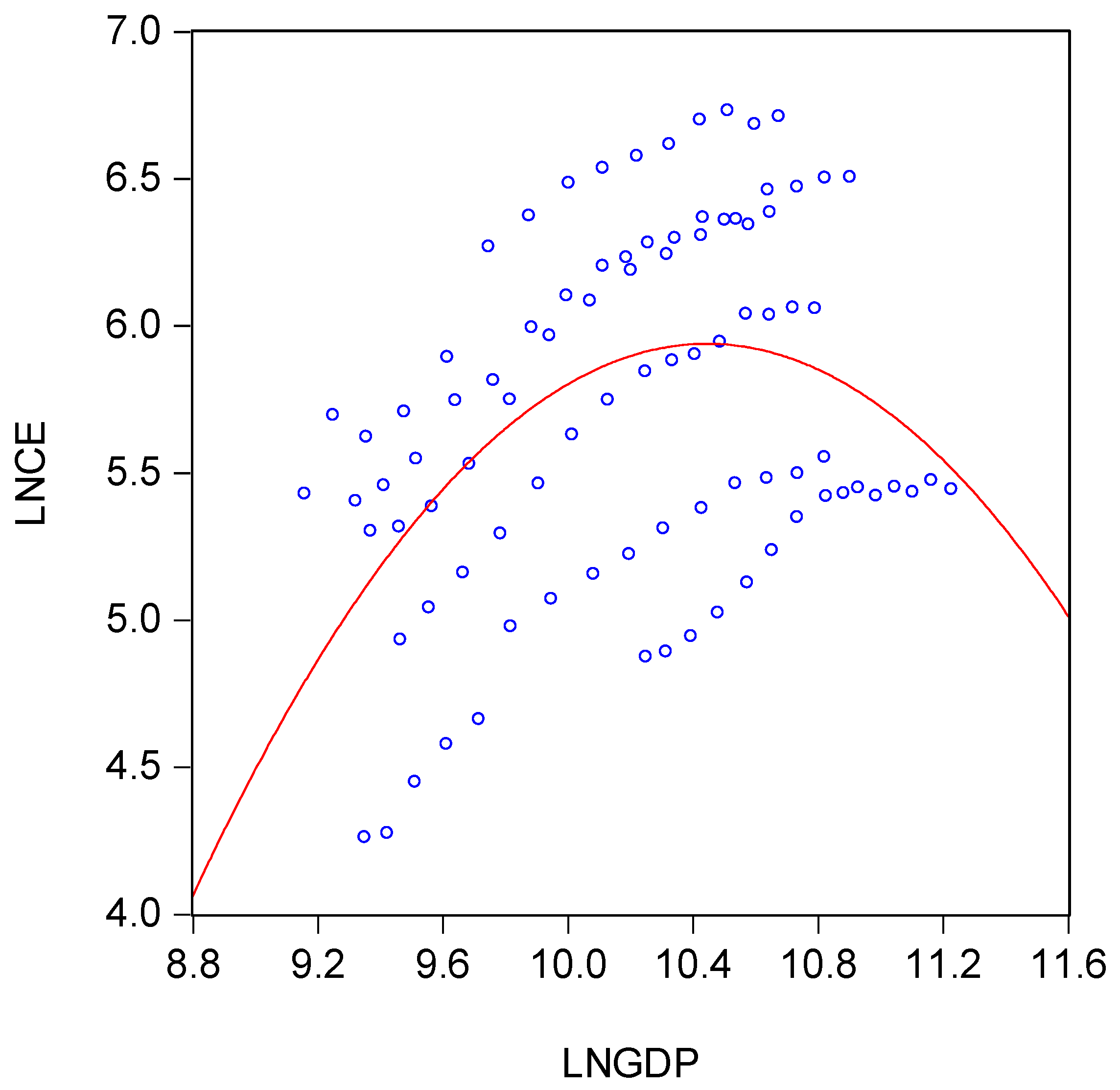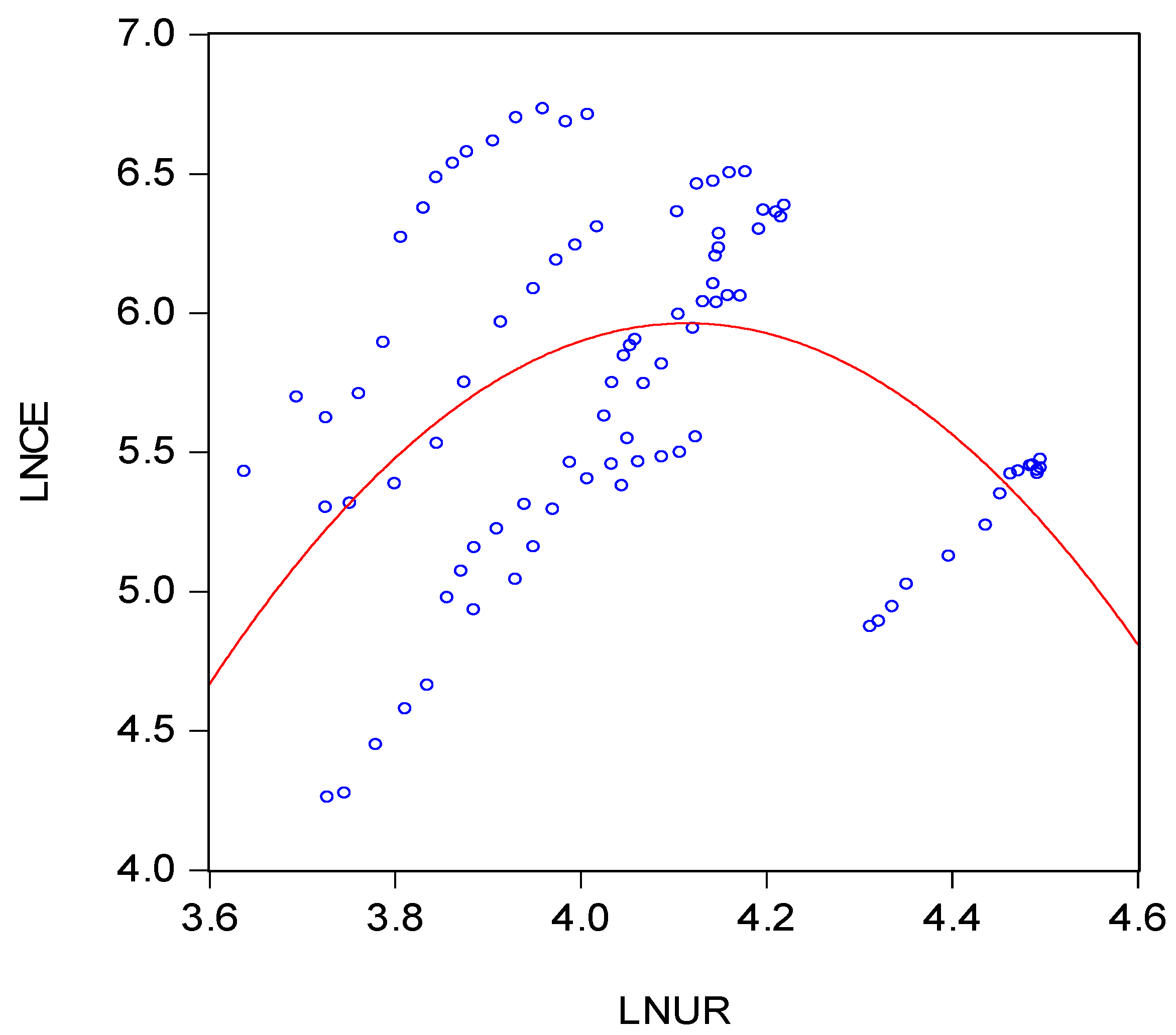[29] studied the EKC relationship and coupling analysis of urbanization and CO₂ emissions in the Yangtze River Delta. Therefore, in order to gain a better understanding of the development level, this paper explored the EKC hypothesis of per capita GDP/urbanization and carbon emissions in the Region.

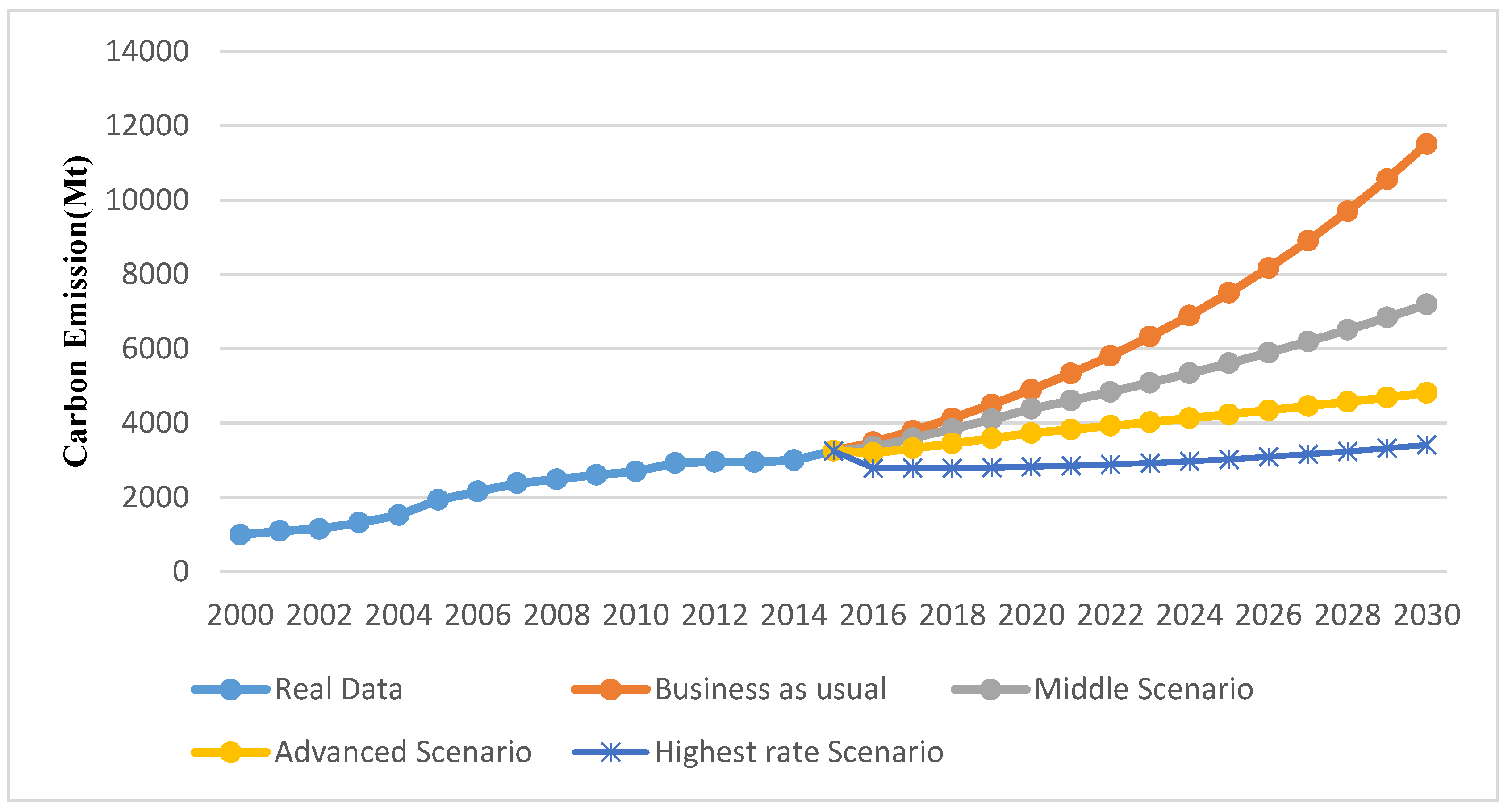
According to the abovementioned research findings, this paper filled in three aspects of the research gap that have not been considered in the existing literature. Firstly, the study selected six provinces in the east and south coastal area as the research object, which played an important role in estimating national carbon emission reduction targets. Only one other article selected this Region as a research object, although it used LMDI to analyze the influence indexes of CO₂ emissions. Because the selected factors of LMDI are limited, the analysis of factors impacting carbon emissions is not comprehensive. In this study, the STIRPAT method was used to study the factors influencing carbon dioxide emissions in the Region, which made up for the limited selection of factors. Also, we verified the EKC hypothesis between per capita GDP/urbanization and carbon emissions in order to further understand the current development stage. Furthermore, taking into account the importance of the Region, this study predicted the contribution of this Region to the national 2020 and 2030 emission reduction targets. Based on the three ordinary scenarios, the highest-rate scenario was innovatively added, based on the highest growth rate of historical data. This scenario served as a basis for reality. Finally, more applicable and effective policy recommendations for reducing CO₂ emissions in the Region were proposed.

3. Methods and Data Description

3.1. Estimation of CO₂ Emissions

Following the 2006 guidelines of the Intergovernmental Panel on Climate Change (IPCC), CO₂ emissions calculated from energy consumption, emission coefficients, and the fraction of oxidized carbon by fuel are as follows [34]:

$${\mathrm{CO}}_{2\mathrm{i}}^{\mathrm{t}}={\displaystyle \sum }_{\mathrm{j}}{\mathrm{CO}}_{2\mathrm{ij}}^{\mathrm{t}}={\displaystyle \sum }_{\mathrm{j}}{\mathrm{E}}_{\mathrm{ij}}^{\mathrm{t}}{\times \mathrm{EF}}_{\mathrm{j}}{\times \mathrm{O}}_{\mathrm{j}}\times \frac{44}{12}$$

(1)

where ${\mathrm{CO}}_{2\mathrm{i}}^{\mathrm{t}}$ denotes the total CO₂ emissions of province $\mathrm{i}$ in year $\mathrm{t}$; ${\mathrm{CO}}_{2\mathrm{ij}}^{\mathrm{t}}$ is the CO₂ emissions for fuel type $\mathrm{j}$ of province $\mathrm{i}$ in year $\mathrm{t}$; ${\mathrm{E}}_{\mathrm{ij}}^{\mathrm{t}}$ refers to the energy consumption of fuel type $\mathrm{j}$ in province $\mathrm{i}$ in year $\mathrm{t}$; ${\mathrm{EF}}_{\mathrm{j}}$ is the CO₂ emission coefficient of fuel type $\mathrm{j}$; and ${\mathrm{O}}_{\mathrm{j}}$ means the fraction of the carbon oxidized of fuel type $\mathrm{j}$.

Because the amount of electricity generated from nuclear power and hydroenergy is rapidly rising, the contribution of nuclear energy and water power to generate electricity cannot be ignored. [35]. The carbon emissions ratios ($\mathrm{ef}$) of heat and electricity can be computed as follows:

$${\mathrm{ef}}_{\mathrm{t}}=\frac{{\sum }_{\mathrm{j}}{\mathrm{CO}}_{2_{\mathrm{j},\mathrm{t}}}}{{\mathrm{E}}_{\mathrm{fossil},\mathrm{t}}{+\mathrm{E}}_{\mathrm{nuclear},\mathrm{t}}{+\mathrm{E}}_{\mathrm{hydro},\mathrm{t}}}$$

(2)

where ${\mathrm{ef}}_{\mathrm{t}}$ refers to the average emission coefficient in year $\mathrm{t}$; ${\mathrm{CO}}_{2_{\mathrm{j},\mathrm{t}}}$ indicates the CO₂ for fossil fuel type $\mathrm{j}$ in year $\mathrm{t}$; and ${\mathrm{E}}_{\mathrm{fossil},\mathrm{t}}$, ${\mathrm{E}}_{\mathrm{nuclear},\mathrm{t}}$, ${\mathrm{E}}_{\mathrm{hydro},\mathrm{t}}$ denote fossil fuel consumption, nuclear energy, and hydropower in year $\mathrm{t}$.

3.2. Empirical Model

Ehrlich and Holdren [36] first proposed the IPAT model to quantify the impact of human activities on the environment.

$$\mathrm{I}=\mathrm{P}\times \mathrm{A}\times \mathrm{T}$$

(3)

where I refers to the environmental impact, P represents population size, A means affluence, and T denotes technological progress. This accounting equation only contains some key factors, which assumes unified elasticity of population, affluence, and technology. Based on IPAT, Dietz and Rosa [37] proposed the STIRPAT model to overcome these limitations:

$${\mathrm{I}=\mathrm{aP}}_{\mathrm{i}}^{\mathrm{b}}{\mathrm{A}}_{\mathrm{i}}^{\mathrm{c}}{\mathrm{T}}_{\mathrm{i}}^{\mathrm{d}}{\mathrm{e}}_{\mathrm{i}}$$

(4)

where $\mathrm{i}=1,2,3,\dots ,N$ represents the cross-section dimension; $\mathrm{a}$ denotes the constant term; $\mathrm{b}$, $\mathrm{c}$, and $\mathrm{d}$ denote the explanatory variable coefficients based on P, A, and T, respectively; $\mathrm{e}$ is the random error term. When a = b = c = d = 1, the IPAT framework is a special form of the STARPAT model [16]. Taking the logarithms of the equation, the model can be represented as follows:

$${\mathrm{lnI}}_{\mathrm{i}}={\mathrm{a}}_{\mathrm{i}}+{\mathrm{blnP}}_{\mathrm{i}}+{\mathrm{clnA}}_{\mathrm{i}}+{\mathrm{dlnT}}_{\mathrm{i}}+{\mathrm{e}}_{\mathrm{i}}$$

(5)

In the STIRPAT model, P, A, and T can be decomposed into a number of factors that affect the environment. For example, T can be replaced by energy structure, energy intensity, and technical progress coefficient [30,38]. Therefore, the STIRPAT model has few constraints on the selection factors. For example, some studies have innovatively selected urbanization factors to study the relationship between urbanization and energy utilization or CO₂ emissions [13,39,40]. In order to research the impact factors of CO₂ emissions more comprehensively, we choose the factors of energy efficiency, industry share, and urbanization to extend the STIRPAT model [13]. The logarithm form of the integrated pattern we adopted is:

$${\mathrm{lnCE}}_{\mathrm{it}}{=\mathsf{\alpha }+\mathsf{\beta }}_1{\mathrm{lnPOP}}_{\mathrm{it}}{+\mathsf{\beta }}_2{\mathrm{lnGDP}}_{\mathrm{it}}{+\mathsf{\beta }}_3{\mathrm{lnUR}}_{\mathrm{it}}{+\mathsf{\beta }}_4{\mathrm{lnEI}}_{\mathrm{it}}{+\mathsf{\beta }}_5{\mathrm{lnIS}}_{\mathrm{it}}{+\mathrm{e}}_{\mathrm{it}}$$

(6)

where i and t represent province and time, respectively; CE means energy-related carbon emissions; POP denotes population; GDP is per capita GDP; EI means energy efficiency, calculated by dividing energy consumption by GDP; UR represents the proportion of urban population to the total population; and IS indicates industrial structure, which is calculated by the proportion of the value of the secondary industry to the GDP.

In order to test the EKC hypothesis, Kang et al. [41] and Sinha and Bhattacharya [42] focused on the relationship between CO₂ emissions and wealth factor, and a quadratic term of per capita GDP was added to the formula. The results showed that there existed an inverted U-shaped Kuznets curve relation between per capita GDP and carbon dioxide emissions. In addition, some scholars studied the EKC hypothesis of CO₂ emissions and demographic variables, which were represented by the urbanization rate [14,33]. Based on the research progress in this field, we obtained two extended STIRPAT models to test inverted U-shape relations between economic growth/urbanization and carbon emissions. Based on the framework of the ECK hypothesis, we transformed the variables into natural logarithm form, and the formula is as follows:

$${\mathrm{lnCE}}_{\mathrm{it}}{=\mathsf{\alpha }+\mathsf{\beta }}_1{\mathrm{lnPOP}}_{\mathrm{it}}{+\mathsf{\beta }}_2{\mathrm{lnGDP}}_{\mathrm{it}}{+\mathsf{\beta }}_3{{(\mathrm{lnGDP}}_{\mathrm{it}})}^2{+\mathsf{\beta }}_4{\mathrm{lnUR}}_{\mathrm{it}}{+\mathsf{\beta }}_5{\mathrm{lnEI}}_{\mathrm{it}}{+\mathsf{\beta }}_6{\mathrm{lnIS}}_{\mathrm{it}}{+\mathrm{e}}_{\mathrm{it}}$$

(7)

$${\mathrm{lnCE}}_{\mathrm{it}}{=\mathsf{\alpha }+\mathsf{\beta }}_1{\mathrm{lnPOP}}_{\mathrm{it}}{+\mathsf{\beta }}_2{\mathrm{lnGDP}}_{\mathrm{it}}{+\mathsf{\beta }}_3{\mathrm{lnUR}}_{\mathrm{it}}{+\mathsf{\beta }}_4{{(\mathrm{lnUR}}_{\mathrm{it}})}^2{+\mathsf{\beta }}_5{\mathrm{lnEI}}_{\mathrm{it}}{+\mathsf{\beta }}_6{\mathrm{lnIS}}_{\mathrm{it}}{+\mathrm{e}}_{\mathrm{it}}$$

(8)

3.3. Data Sources and Description

3.3.1. Data Sources

In the study, we applied the panel data of six provinces from 2000 to 2015. The expenditure of energy was acquired from the China Energy Statistic Yearbook [9]. This study considered 18 types of fuel, including raw coal, cleaned coal, washed coal, coke, coke oven gas, other gas, crude oil, gasoline, kerosene, diesel oil, fuel oil, liquefied petroleum gas (LPG), refinery gas, natural gas, other petroleum, other coking products, electricity, and heat.

The provincial population, per capita GDP, urbanization, and the proportion of the value of the secondary industry to the GDP were obtained from the China Statistical Yearbook [8]. GDP data were converted to 2000 constant price, calculated with provincial GDP deflation factors. Variable definitions and units are listed in

Table 1. Description of variables used in the analysis for the period of 2000–2015 [43].

Variables	Definition	Unit of Measurement
CO2 Emissions (CE)	Energy-related CO2 emissions	Million tons
Population (POP)	Population at the end of the year	104 units
Urbanization (UR)	The percentage of the urban population in the total population	%
GDP Per Capita (GDP)	GDP divided by population at the end of the year	Yuan in 2000 constant price
Energy Intensity (EI)	Total energy use divided by GDP	Tce per 104 yuan
Industrial Structure (IS)	The percentage of the secondary industry GDP in the total industry GDP	%

.

3.3.2. Data Description

Figure 1 illustrates the changing rate of the variables, with 2000 as the base year. As can be seen from the figure, most of the variables were non-stationary. During the study period, they continued to rise, fall, or exhibit horizontal fluctuations. Among these variables, per capita GDP rose almost to three times the original amount with the fastest growth rate, followed by carbon emissions, which increased by two times the original amount. As the energy intensity was reduced by less than 50%, we can see that energy consumption rose to almost twice the original amount. Although the growth rate of industrial structure was not significant, the Region’s second industry GDP accounted for half of the country; thus, the influence of this factor cannot be ignored [8]. According to the trend of CO₂ emissions, it can be seen that the growth rate has increased dramatically since 2001. This was because China acceded to the World Trade Organization in 2001, which led a substantial rise in consumption and exports, in turn resulting in a comprehensive rise in carbon emissions [44]. The growth rate then began to slow in 2005, mainly due to the world economic crisis and the effective implementation of energy-saving and emission-reduction policies in the “11th Five-Year Plan” [5,45].

4. Results and Discussion

4.1. Panel Unit Root and Co-Integration Tests

Ordinarily, most economic variable sequences are not stationary. If non-stationary variable sequences were brought into the economic model, the result of regression was not reliable. Therefore, we needed use the unit root test to estimate the robustness of variable sequences. We employed the first-order differencing method to transform non-stationary sequences into stationary sequences [43]. Based on panel data, the econometric theory provides many unit root tests. As IPS, Fisher-ADF, and Fisher-PP tests have been widely used, in this study we also chose these methods to test the panel unit root [43,46]. Unit root test results for the explanatory and dependent variables are shown in

Table 2. Results of panel unit root tests using the IPS test, Fisher-ADF test, and Fisher-PP test in 1st difference [47].

Variable	IPS	Fisher-ADF	Fisher-PP
Carbon Dioxide Emissions	−0.784 **	14.331 **	24.460 ***
Population	−1.228 ***	20.151 ***	27.974 ***
Urbanization	−1.838 ***	20.963 ***	58.609 ***
Urbanization-Square	−1.547 ***	19.759 ***	51.622 ***
GDP Per Capita	−1.840 ***	21.848 ***	49.989 ***
GDP Per Capita-Square	−2.751 ***	28.217 ***	51.337 ***
Energy Intensity	−1.828 **	21.910 **	48.306 ***
Industrial Structure	−1.375 ***	18.727 ***	30.135 ***

Note: ** and *** donate that the variable is significant at the 5% and 1% level, respectively.

. The results showed that most of the variables were non-stationary. However, the results of their first-order difference strongly rejected the null hypothesis. It was shown that the first-order difference sequences were stationary. Next, we performed the co-integration test.

We used bivariate and residual-based co-integration tests to examine the relation. Outcomes are listed in

Table 3. Testing for bivariate co-integration between the CO₂ emissions level and its influencing factors [43].

Test Statistics	POP	UR	UR2	GDP	GDP2	EI	IS
Panel v-Statistic	0.569 ***	1.941 ***	1.851 ***	0.486 **	6.608 ***	73.483 ***	16.679 ***
Panel rho-Statistic	−0.351 ***	−1.008 ***	−0.597 ***	0.929 *	1.053 *	0.983 *	1.583 *
Panel PP-Statistic	−0.868 ***	−1.312 ***	−0.691 ***	−0.474 **	−1.425 ***	−0.806 **	−0.017 **
Panel ADF-Statistic	−0.621 ***	−2.454 ***	−2.180 ***	−2.603 ***	−2.892 ***	−3.551 ***	−1.597 ***
Group rho-Statistic	1.278 *	1.092 *	1.386 *	1.646 *	1.599 *	2.361 *	1.901 **
Group PP-Statistic	0.104 **	0.198 **	0.719 *	0.018 **	−1.088 ***	1.412 *	0.152 **
Group ADF-Statistic	−0.441 ***	−2.404 ***	−2.256 ***	−3.458 ***	−3.686 ***	−1.884 ***	−0.380 ***
Residual-Based Tests for Co-integration [48]
Variable	Coefficient		Std. Error		T-Statistic		Prob.
RESID(−1)	−0.183		0.076		−2.396		0.019
D(RESID(−1))	0.263		0.128		2.053		0.044
D(RESID(−2))	0.221		0.132		1.685		0.001
ADF	−1.137 ***

Note: Lags are all selected automatically by AIC and SC standard. ADF is the test statistics developed by Kao [48]; ***, **, and * represent a significance of 1%, 5%, and 10%, respectively.

. The bivariate co-integration test presented here was a co-integration relation between CO₂ emissions and its explanatory variables. The residual-based co-integration test was developed by Reference [48]. The results showed that the ADF statistic was −1.137, which strongly rejected the null hypothesis that there was no co-integration among all variables. Therefore, a co-integration relation was identified between the CO₂ emissions level and its driving factors.

4.2. Multicollinearity Testing

In the multivariate regression model, the regression results are not reliable if there is a strong linear correlation between variables. Thus, it is necessary to verify the multicollinearity of independent variables before the regression model is calculated [49]. We used the variance inflation factor (VIF) method to test the multicollinearity of variables. Generally speaking, if the VIF value is greater than 10, serious multicollinearity among variables is indicated [16]. The multicollinearity test results are shown in

Table 4. Multicollinearity test of the variables used in the study [49].

Variable	VIF	VIF	VIF
LnPOP	4.390	4.632	4.991
LnUR	4.215	205.540	4.240
(LnUR)2		212.730
LnGDP	5.258	7.302	255.306
(LnGDP)2			242.975
LnEI	1.331	1.532	1.383
LnIS	5.638	8.369	7.668

. In our study, the large VIF values of urbanization and squared urbanization, GDP per capita and squared GDP per capita were inevitable. The results showed that there was no multicollinearity among independent variables except the quadratic term.

4.3. Heteroscedasticity and Robust Regression

The multiple regression model assumes that random errors have the same variance as independent variables. If the assumption is not satisfied, the multiple regression model has heteroscedasticity. If heteroscedasticity exists, the ordinary least squares model cannot be effectively estimated. The White test was applied to examine heteroscedasticity. If the null hypothesis is that the error term has heteroscedasticity, and if the p value is less than 0.1, it is shown that heteroscedasticity can affect the validity of the orthogonal least squares (OLS) results [49].

Generally speaking, we can use the robust regression to solve the heteroscedasticity problem. According to the results of OLS, robust regression removes the extreme observations and calculates the weights based on the residual observations. These weights are used to compute the robust least squares regression. Through repeating this procedure, the weight of the extreme value is reduced to the minimum. That is, after extreme values are removed, the results of the robust regression and OLS are most similar [50].

4.4. Estimation Results

In order to avoid multicollinearity, we employed three regression models in

Table 5. The results of Robust Regression A, B, C, and OLS Regression [49].

Variables	Robust Regression A	OLS Regression	Robust Regression B	Robust Regression C
C	−12.219 ***	−12.202 **	−13.970 ***	−15.748 ***
LnPOP	0.945 ***	0.946 ***	0.950 ***	0.949 ***
LnUR	0.076 ***	0.073 *	−0.076 ***	1.849 ***
(LnUR)2				−0.219 ***
LnGDP	0.824 ***	0.825 **	1.179 ***	0.845 ***
(LnGDP)2			−0.017 ***
LnEI	0.865 ***	0.868 *	0.860 ***	0.877 ***
LnIS	0.368 ***	0.361 **	0.339 ***	0.295 ***
Heteroscedasticity	Yes	Yes	Yes	Yes
R-squared	0.876	0.897	0.894	0.865
Observations	90	90	90	90

The symbol * represents p < 0.1; ** represents p < 0.05; *** represents p < 0.01.

[43]. After a STIRPAT model was established, robust regression and OLS regression were conducted to analyze and compare the results. Model A was used to examine five major carbon emission drivers, while models B and C were used to verify the EKC relation about economic growth/urbanization and CO₂ emissions. Due to the regression models with heteroscedasticity, the elasticities of various factors in the robust regression were more significant, compared to OLS. Therefore, robust regression was more reliable. The results showed that all of the coefficients were positive, which indicated that the five main factors were positively correlated with carbon emissions. Among them, population size had the most positive influence on CO₂ emissions [49]. The coefficients of per capita GDP and energy efficiency were relatively higher. The elasticities were 0.824 and 0.865, respectively, which meant that if per capita GDP experienced a growth of 1%, carbon emissions would increase by 0.824%, and every 1% growth of energy intensity would result in an increase in carbon emissions of 0.865%. The positive impact of industry share on CO₂ emissions was relatively small, followed by the effect of urbanization.

According to the result of model B, the coefficient of ln(GDP) was positive, while the square coefficient of ln(GDP) was remarkably less than zero, confirming the inverse U-shaped relation between per capita GDP and CO₂ emissions. According to Figure 2, the six provinces have substantially exceeded the critical inflection point. The logical support to the EKC theory is that environmental quality is expensive and the rich can afford it; that is, the impact of GDP growth on the environment shows a significant scale effect. In addition to this effect, once the society becomes rich enough, people pay more attention to the environment, so they can put money into new Research and Development (R&D) technology and efficient low-carbon technology. The society can thus effectively use related approaches that greatly improve environmental issues [14,51,52,53].

According to the results of model C, the coefficient of urbanization was positive, and its square terms were significantly negative, indicating that there also existed an inverted U-shape Kuznets curve relation between urbanization and carbon emissions. Figure 3 shows that the six provinces have substantially reached this critical inflection point. The reason for this phenomenon is that the six provinces in the Region are developed provinces with a high economic development level; therefore, they have funds invested in the research and development of low-carbon technology, so as to achieve the purpose of energy conservation and emission reduction. When past a turning point, the growth of urbanization rate will play a role in inhibiting carbon emissions. This contradicted many previous studies, although it is consistent with the theory of ecological modernization [33,54,55,56].

4.5. Scenario Analysis

4.5.1. Scenario Setting

Figure 4 shows that the trends of the real value and the estimated value were basically the same, indicating that the results of the curve fitting were very satisfactory. According to the relationship between variables, four scenarios were set up to predict the contribution of the Region to the national 2020 and 2030 reduction targets.

In the business as usual (BAU) scenario, the average growth rate of all variables can be derived from historical data. Under these circumstances, this study assumed that the variables growth rate, technical and policy factors do not change.

In the highest-rate scenario (HS), the optimal rates of GDP per capita, energy efficiency, and industrial structure were selected, as obtained from the data of 2000–2015. Considering the necessity of controlling variables, the growth rates of the remaining variables were the same as those in the BAU scenario. The advanced scenario (AS) referred to the optimal situation of carbon emission reduction. Considering the significant role of per capita GDP and energy efficiency, in this context, the growth rates of the two factors were set according to national policy. According to the “13th Five-Year Plan”, the annual GDP growth rate was expected to be 6.5%, and energy intensity would be reduced by 15% in 2020, compared to 2015 [4]. This study designed the annual growth rate of the industrial structure according to Reference [27]. The annual growth rates of other factors were calculated from historical data.

For the middle scenario (MS), the changing trend of three variables was within the thresholds of the BAU and advanced scenarios. The change rates of variables in different scenarios are shown in

Table 6. Assumptions of the growth rate of each variable under different scenarios in 2020 and 2030 (%).

Variables	Year	GDP	EI	IS
BAU(Business As Usual)	2020	10.2	−1.94	2.13
	2030	10.2	−1.94	2.13
MS(Middle Scenario)	2020	8.5	−2	1.26
	2030	7.5	−3	1.09
AS(Advanced Scenario)	2020	6.5	−3	0.40
	2030	6	−4	0.13
HS(Highest-rate Scenario)	2020	7.7	−9.3	−4.5
	2030	7.7	−9.3	−4.5

.

4.5.2. Result Analysis in BAU

In the BAU, carbon emissions, overall GDP, and carbon intensity are shown in

Table 7. The carbon emissions, GDP, and carbon intensity under the basic scenario [8,9].

Year	Carbon Emissions (Mt)	Total GDP (BY, 2000 Constant Price)	Carbon Intensity (Mt/BY)
2005	1930.863	75,286.657	0.0256
2010	2695.567	136,938.718	0.0197
2015	3252.213	217,610.824	0.0149
2020	5009.989	379,141.086	0.0132
2025	7723.648	660,954.555	0.0117
2030	11,915.639	1,152,883.379	0.0103

. According to the trend of variables from 2000 to 2015, we learned that CO₂ emissions and GDP continued to rise, while the carbon intensity began to decline in 2005, because the growth rate of GDP was higher than that of carbon emissions. According to the relationship between the variables in the robust regression results, we calculated that carbon emissions would reach 5009.989 Mt in 2020 and 11,915.639 Mt in 2030, which were five times and 12 times that in 2000, respectively. The carbon intensities for 2020 and 2030 would be 0.0132 Mt/BY and 0.0103 Mt/BY, respectively, which were 48.5% and 59.7% lower than that in 2005.

Although this scenario barely reached the national emission reduction targets, the degree of carbon emission reduction was not enough for developed provinces in China. However, although the Region’s CO₂ emissions accounted for one third of the total CO₂ emissions of China, considering its higher proportion of the GDP, the carbon intensity of this Region was not too high. On the contrary, some less-developed provinces in China exhibited high carbon emissions and low economic levels, resulting in high carbon intensity, such as Qinghai, Ningxia, Shanxi, Xinjiang, etc. [8,9]. These provinces face more obstacles to reducing carbon emissions, so we should make greater efforts to reduce carbon emissions in developed areas.

In Figure 5, showing the comparison of GDP and carbon emissions in the provinces in 2000 and 2015, it is clearly indicated that obvious differences exist between the development degrees of the provinces. Shanghai and Guangdong were in the best condition; although carbon emissions grew in these areas, but the growth of the GDP was more significant. Shandong was in the worst state; during the study period, this province saw the largest increase in carbon emissions, but its GDP was lower than that of Jiangsu. Jiangsu, Zhejiang, and Fujian were at the medium level, and there was still room for carbon reductions. The development level of the six provinces was consistent at a certain level, but slight differences existed among them. Therefore, a better strategy was to implement different emission reduction strategies after classifying each province [5,16,17,57,58,59].

4.5.3. Results Analysis in Alternative Scenarios

Carbon emissions, total GDP, and energy intensity in four scenarios are presented in

Table 8. The carbon emissions, GDP, and carbon intensity in 2005, 2020, and 2030 under the basic and alternative scenarios.

Year	Scenarios	Carbon Emissions (Mt)	Total GDP (BY, 2000 Constant Price)	Carbon Intensity (Mt/BY)
2005		1930.863	75,286.657	0.0256
2020	BAU	5009.989	379,141.086	0.0132
	MS	4441.513	340,303.909	0.0131
	AS	3769.352	304,359.004	0.0124
	HS	2820.229	326,171.816	0.0086
2030	BAU	11,915.640	1,152,883.379	0.0103
	MS	7286.190	789,614.567	0.0092
	AS	4861.695	613,632.537	0.0079
	HS	3413.714	771,345.297	0.0044

. In general, with the implementation of targeted measures, CO₂ emissions would be substantially decreased. In the middle scenario, emissions mitigation was not significant in 2020, as it was only decreased by 568.476 Mt compared to the BAU scenario, and the carbon intensity was reduced by 49.11% compared to 2005. Carbon emissions in 2030 decreased significantly by 4629.45 Mt, compared with the basic scenario, and carbon intensity decreased by 64.02% compared to 2005. As a result, carbon intensity had greater contribution to carbon emission reduction in 2030.

In the advanced scenario, carbon emissions in 2020 were expected to reach 3769.352 Mt, which would respectively reduce by 1240.637 Mt and 672.161 Mt compared to the BAU and middle scenarios. Based on the growth rate shown in Table 6, the large gap between the advanced scenario and the BAU scenario was mainly due to a decline in the proportion of the secondary industry GDP. In addition, the carbon intensity in 2020 decreased by 51.71% compared to 2005. Carbon emissions in the advanced scenario in 2030 was significantly lower than those in the middle scenario and basic scenario, and carbon intensity in 2030 decreased by 69.11% compared to 2005. This showed that the expected growth rates of the total GDP, energy intensity, and industrial structure to achieve carbon intensity reduction targets were effective, and would contribute greatly to the national emission reduction targets. In the highest-rate scenario, based on the historical optimal rate of factors, the total carbon emissions were only 2820.229 Mt and 3413.714 Mt in 2020 and 2030, respectively, and the carbon intensity in the Region was expected to reduce by 66.29% in 2020 and 82.74% in 2030. The carbon intensity was effectively mitigated in this scenario, mainly due to a significant reduction in energy intensity and industrial structure. The result far exceeded the expected results in the advanced scenario and provided a realistic basis for the region to overfulfil the national carbon emission reduction targets.

Figure 6 illustrates the carbon emissions of the Region. It shows that in the four scenarios, carbon emissions continued to decrease with the severity of the predictive factors. Further, it was clearly shown that in the advanced scenario, the greatest degree of carbon reduction was achieved compared to the BAU scenario. In addition, emission reduction potential in the Region was represented by the gap of carbon emissions.

4.6. Discussion

As in previous studies, the population was the most prominent factor in the Region. However, because the population size was stable, it had little effect on carbon emissions [13,49]. Similarly, the impact of urbanization on carbon emissions was also very small. As China recently underwent an important period of industrialization and urbanization, in the studied Region representing the country’s cluster of most developed provinces, the impact of economic factors on carbon emissions was obvious. The degree of influence of the per capita GDP was great; moreover, it increased by almost three times during the study period, mainly due to its unique geographical advantages with a high proportion of foreign trade. Therefore, GDP growth was the major driving index of carbon emissions [5,12,13]. Industrial structure also had a great role in increasing carbon emissions. The Region’s manufacturing output accounted for 70% of the country’s total output. Because the manufacturing industry is a high energy consumption and high pollution industry, it was necessary to adjust the industrial structure according to a series of existing policies, such as the Guidance Catalogue of Industrial Structure Adjustment [60,61]. Energy intensity and economic growth had the same importance for carbon emissions, but carbon emissions were inhibited because energy intensity was at a reduced stage. Although energy intensity continued to decline, the total energy consumption still grew rapidly. It is worth noting that thermal power accounts for 20% of the total energy consumption [9]. New energy generation can effectively reduce the consumption of fossil fuels.

For the study of the EKC hypothesis, some studies conducted in-depth investigation of the curve trend between GDP/urbanization and carbon emissions across the country [31,33]. This study confirmed that per capita GDP and CO₂ emissions had an inverted U-shaped relation, which met the logic support EKC hypothesis, and the development period was found to be over the vertex in the decline stage [14]. Also, urbanization and carbon emissions had an inverted U-shaped Kuznets relationship, which met the ecological modernization theory, and the development period was found to be at the peak of the curve [33]. The increase in the level of economy and urbanization has provided conditions for the introduction and effective implementation of environmental policies.

A large number of previous research studies focused on predicting the national carbon emission reduction potential [4,62], though few predicted regional carbon emissions. The Region contains six of the most developed provinces of the country, and it was very meaningful to predict its contribution to the country’s 2020 and 2030 emission reduction targets. This indicated the possibility that China can achieve its emission reduction targets. For the basic scenario, the Region was barely able to complete the carbon emission reduction targets. However, in the advanced scenario, it clearly achieved its goals and contributed greatly to the country’s emission reduction. Also, the result in the highest-rate scenario provided a realistic basis for the region to overfulfil the national carbon emission reduction targets. According to the result, it is necessary to take steps to reduce CO₂ emissions, such as through new energy generation and the adjustment of industrial structure. Due to differences in the development level among provinces, different strategies should be adopted for different provinces [5,58].

5. Conclusions and Policy Implications

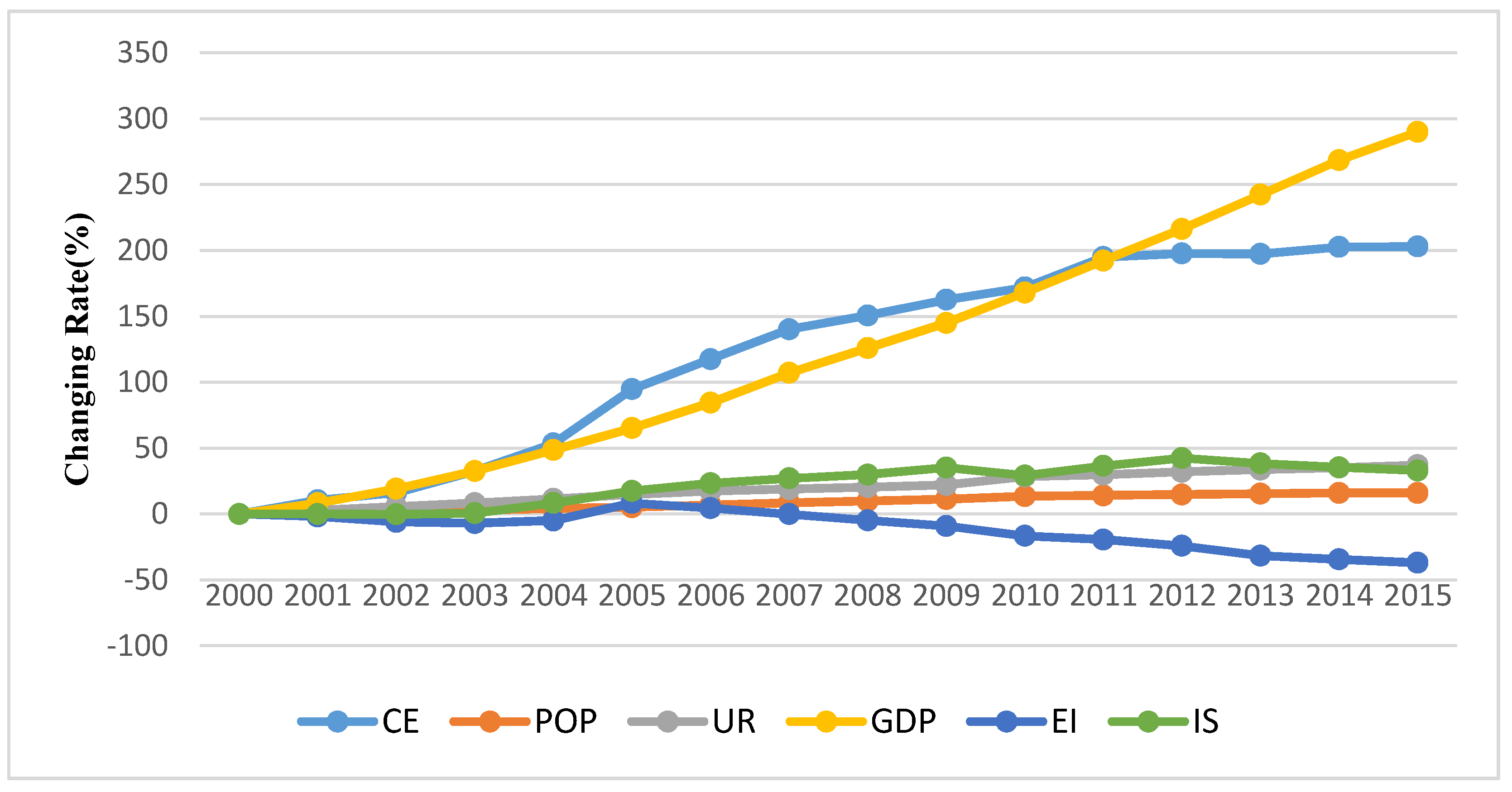
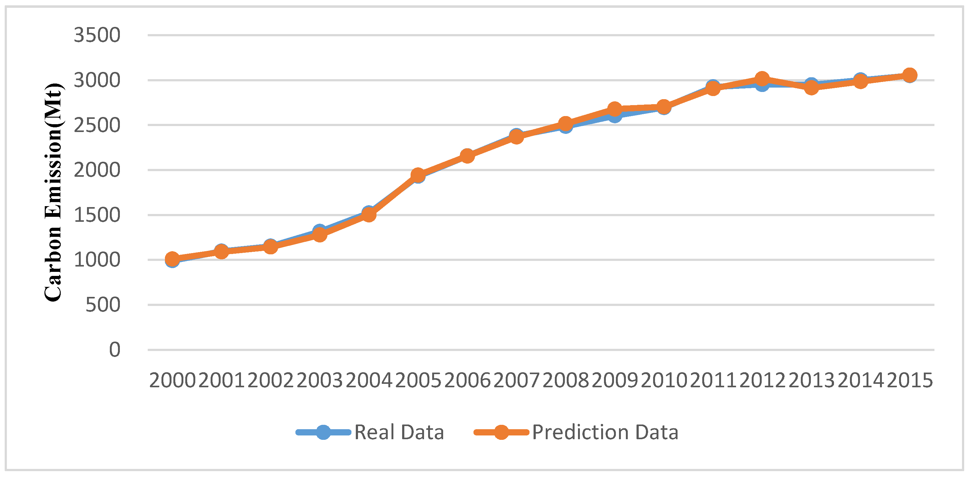
This paper conducted a multivariate analysis of carbon emissions in east and south coastal China from 2000–2015, an area that includes six provinces named Shandong, Zhejiang, Jiangsu, Fujian, Shanghai, and Guangdong. We used the extended STIRPAT model to study impact indexes of carbon emissions. The factors included population, per capita GDP, urbanization, energy efficiency, and industrial structure. What is more, in order to understand the development status more comprehensively, we further verified the EKC hypothesis between per capita GDP/urbanization and carbon emissions. Finally, we forecasted carbon intensity in this area and identified its contribution to the national emission reduction targets in 2020 and 2030. Considering the significance of per capita GDP, energy intensity, and industrial structure obtained from regression results, four scenarios were set to predict the carbon emissions of the area according to the respective growth rates of three factors.

The regression results showed that the population was the most prominent factor. Its change trend was steady, so it had little impact on carbon emissions. Economic growth played a significant role in increasing carbon emissions, while energy intensity was mainly responsible for reducing it. The negative effect of industrial structure was not obvious, so there was a much room for improvement. As for the EKC hypothesis, the relationship between per capita GDP/urbanization and carbon emissions exhibited an inverted U-shape, which can satisfy the logical support EKC hypothesis and ecological modernization theory. Analysis results showed that, in the BAU scenario, the carbon intensity was reduced by 48.5% in 2020 and 59.7% in 2030 compared to 2005, but in the advanced scenario, the carbon intensity was reduced by 51.7% in 2020 and 69.1% in 2030 compared to 2005, which contributed greatly to the national carbon emission reduction targets. From the highest-rate scenario, it can be seen that improving energy efficiency, optimizing energy structure, and adjusting industrial structure can effectively reduce carbon intensity.

Based on the results mentioned above, the future strategies of carbon emission mitigation for policymakers are provided below:

(1) Increasing the emission reduction effect of energy efficiency. Looking to the future, the Region’s GDP will maintain fast growth. It was unreasonable to decrease CO₂ emissions by decreasing the GDP growth rate. Admitting this fundamental problem meant we need to take other measures to reduce CO₂ emissions. Energy efficiency and per capita GDP were the significant factors affecting carbon emissions, but the reduction of energy intensity had yet to be strengthened. Technological progress and innovation can greatly improve energy efficiency, and we should be committed to developing and introducing advanced technology.

(2) Optimizing the energy structure is imminently needed. The energy structure of the Region is dominated by coal. In order to reduce environmental pollution, the Region can continue to optimize the energy structure. It should minimize the proportion of coal in energy use, and speed up the innovation of coal-utilization technology, such as clean coal technology, as well as increase the use of oil, natural gas, and other clean energy. In addition, the Region should vigorously encourage new energy power generation methods, such as solar, hydro, wind, nuclear, and biomass energy generation. As the Region’s main generating power is thermal, the fuel consumption of thermal power accounted for 50% of total fuel consumption; this should be considered as a serious issue.

(3) Encouraging the optimization of industrial structure. It was found that industrial structure remarkably decreased CO₂ emissions in the MS and AS. Although the Region includes the six most developed provinces in the whole country, the proportion of secondary industry GDP is still rising year by year. The Region’s secondary industry accounted for 50% of the national secondary industry GDP, while the manufacturing industry output accounted for more than 70% of the country’s GDP. Enterprises with high consumption, pollution, and carbon emissions were the major sources of CO₂ emissions. Hence, in order to create green ecological cities, it is very important to transform and upgrade industrial structure. Innovative technologies should be advocated in existing industries, while green energy-saving industries could energetically advance the effectiveness of resource distribution and improve fuel utilization. What is more, many Chinese companies do not realize the mutual benefit of decreasing emissions by cooperation with other companies. Especially for high energy-consuming industries, enterprises should realize that energy conservation and environmental protection can be achieved by industrial symbiosis. In addition, due to the different development levels of the six provinces in the Region, different strategies should be adopted for different provinces.

This paper provided a new avenue through which researchers can further explore carbon emissions in specific areas. The EKC curve combined with the econometric model was used to explore the relationship between per capita GDP/urbanization and carbon emissions in specific areas. Based on the traditional scenario settings, the highest-rate scenario was added to predict carbon emissions more comprehensively. However, there are some limitations in this study. Although our current research results are encouraging, we tend to be cautious. In the respect, we look forward to further study, including new indexes and different angles, to conduct a more in-depth investigation of the carbon impact factors in the Region. Meanwhile, there are certain limitations to the study of specific areas to assess whether the national carbon reduction targets can be achieved.

References

1. BP. BP Statistical Review of World Energy Market. Available online: http://www bpcom/content/dam/bp/pdf/energy-economics/statistical-review-2015/bpstatistical-review-of-world-energy-2015-full-reportpdf (accessed on 16 March 2018).
2. IPCC. Mitigation of Climate Change (2014) Working Group III Contribution to the Fifth Assessment Report of IPCC Fifth Assessment Report; UK Cambridge University Press: Cambridge, UK, 2014. [Google Scholar]
3. Kang, J.; Zhao, T.; Liu, N.; Zhang, X.; Xu, X.; Lin, T. A multi-sectoral decomposition analysis of city-level greenhouse gas emissions: Case study of Tianjin, China. Energy 2014, 68, 562–571. [Google Scholar] [CrossRef]
4. Wang, J.; Zhao, T.; Wang, Y. How to achieve the 2020 and 2030 emissions targets of China: Evidence from high, mid and low energy-consumption industrial sub-sectors. Atmos. Environ. 2016, 145, 280–292. [Google Scholar] [CrossRef]
5. Gao, C.; Liu, Y.; Jin, J.; Wei, T.; Zhang, J.; Zhu, L. Driving forces in energy-related carbon dioxide emissions in east and south coastal China: Commonality and variations. J. Clean. Prod. 2016, 135, 240–250. [Google Scholar] [CrossRef]
6. Song, M.; Guo, X.; Wu, K.; Wang, G. Driving effect analysis of energy-consumption carbon emissions in the Yangtze River Delta region. J. Clean. Prod. 2015, 103, 620–628. [Google Scholar] [CrossRef]
7. Yu, X.; Yuan, Z.; Fung, J.C.H.; Xue, J.; Li, Y.; Zheng, J.; Lau, A.K.H. Ozone changes in response to the heavy-duty diesel truck control in the Pearl River Delta. Atmos. Environ. 2014, 88, 269–274. [Google Scholar] [CrossRef]
8. National Bureau of Statistics of China (NBSC). Chinese Statistical Yearbook; China Statistics Press: Beijing, China, 2001–2016. [Google Scholar]
9. National Bureau of Statistics of China (NBSC). China Energy Statistical Yearbook; China Statistics Press: Beijing, China, 2001–2016. [Google Scholar]
10. Zhang, M.; Li, H.; Zhou, M.; Mu, H. Decomposition analysis of energy consumption in Chinese transportation sector. Appl. Energy 2011, 88, 2279–2285. [Google Scholar] [CrossRef]
11. Meng, M.; Jing, K.; Mander, S. Scenario analysis of CO2 emissions from China’s electric power industry. J. Clean. Prod. 2017, 142 Pt 4, 3101–3108. [Google Scholar] [CrossRef]
12. Zhang, C.; Tan, Z. The relationships between population factors and China’s carbon emissions: Does population aging matter? Renew. Sustain. Energy Rev. 2016, 65, 1018–1025. [Google Scholar] [CrossRef]
13. Zhou, Y.; Liu, Y. Does population have a larger impact on carbon dioxide emissions than income? Evidence from a cross-regional panel analysis in China. Appl. Energy 2016, 180, 800–809. [Google Scholar] [CrossRef] [Green Version]
14. Wang, Y.; Han, R.; Kubota, J. Is there an Environmental Kuznets Curve for SO2 emissions? A semi-parametric panel data analysis for China. Renew. Sustain. Energy Rev. 2016, 54, 1182–1188. [Google Scholar] [CrossRef]
15. Wang, Y.; Zhao, T. Impacts of energy-related CO2 emissions: Evidence from under developed, developing and highly developed regions in China. Ecol. Indic. 2015, 50, 186–195. [Google Scholar] [CrossRef]
16. Wang, P.; Wu, W.; Zhu, B.; Wei, Y. Examining the impact factors of energy-related CO2 emissions using the STIRPAT model in Guangdong Province, China. Appl. Energy 2013, 106, 65–71. [Google Scholar] [CrossRef]
17. Xu, S.-C.; Zhang, L.; Liu, Y.-T.; Zhang, W.-W.; He, Z.-X.; Long, R.-Y.; Chen, H. Determination of the factors that influence increments in CO2 emissions in Jiangsu, China using the SDA method. J. Clean. Prod. 2017, 142 Pt 4, 3061–3074. [Google Scholar] [CrossRef]
18. Xu, X.; Zhao, T.; Liu, N.; Kang, J. Changes of energy-related GHG emissions in China: An empirical analysis from sectoral perspective. Appl. Energy 2014, 132, 298–307. [Google Scholar] [CrossRef]
19. Yan, Q.; Zhang, Q.; Zou, X. Decomposition analysis of carbon dioxide emissions in China’s regional thermal electricity generation, 2000–2020. Energy 2016, 112, 788–794. [Google Scholar] [CrossRef]
20. Guo, Y.G.; Lin, F.C.; Bai, Y.Q.; Wu, M.M. The decomposition research on energy-related carbon emissions of Shanghai. Environ. Pollut. Control 2009, 7, 18. [Google Scholar]
21. Liu, C.; Chen, C.; Chen, Q.; Zhu, S.; Wang, H.; Zheng, L.I. Evolution Mechanisms of CO2 Emissions in Beijing City during the Period 1997–2007. Resour. Sci. 2010, 32, 235–241. [Google Scholar]
22. Xin, Z. The Status and Decomposition Model of Carbon Emissions for Jiangsu Province. China Popul. Resour. Environ. 2010, 20, 25–30. [Google Scholar]
23. Liu, L.-C.; Fan, Y.; Wu, G.; Wei, Y.-M. Using LMDI method to analyze the change of China’s industrial CO2 emissions from final fuel use: An empirical analysis. Energy Policy 2007, 35, 5892–5900. [Google Scholar] [CrossRef]
24. Lin, B.; Zhao, H. Energy efficiency and conservation in China’s chemical fiber industry. J. Clean. Prod. 2015, 103, 345–352. [Google Scholar] [CrossRef]
25. Xie, X.; Shao, S.; Lin, B. Exploring the driving forces and mitigation pathways of CO2 emissions in China’s petroleum refining and coking industry: 1995–2031. Appl. Energy 2016, 184, 1004–1015. [Google Scholar] [CrossRef]
26. Salahuddin, M.; Alam, K.; Ozturk, I. The effects of Internet usage and economic growth on CO2 emissions in OECD countries: A panel investigation. Renew. Sustain. Energy Rev. 2016, 62, 1226–1235. [Google Scholar] [CrossRef]
27. Tan, X.; Dong, L.; Chen, D.; Gu, B.; Zeng, Y. China’s regional CO2 emissions reduction potential: A study of Chongqing city. Appl. Energy 2016, 162, 1345–1354. [Google Scholar] [CrossRef]
28. Grossman, G.M.; Krueger, A.B. Economic Growth and the Environment. Q. J. Econ. 1995, 110, 353–377. [Google Scholar] [CrossRef]
29. Zhao, Y.; Wang, S.; Zhou, C. Understanding the relation between urbanization and the eco-environment in China’s pearl River Delta using an improved EKC model and coupling analysis. Sci. Total Environ. 2016, 571, 862–875. [Google Scholar] [CrossRef] [PubMed]
30. York, R.; Rosa, E.A.; Dietz, T. STIRPAT, IPAT and ImPACT: Analytic tools for unpacking the driving forces of environmental impacts. Ecol. Econ. 2003, 46, 351–365. [Google Scholar] [CrossRef]
31. Diao, X.D.; Zeng, S.X.; Tam, C.M.; Tam, V.W.Y. EKC analysis for studying economic growth and environmental quality: A case study in China. J. Clean. Prod. 2009, 17, 541–548. [Google Scholar] [CrossRef]
32. Ouyang, X.; Lin, B. Carbon dioxide (CO2) emissions during urbanization: A comparative study between China and Japan. J. Clean. Prod. 2017, 143, 356–368. [Google Scholar] [CrossRef]
33. He, Z.; Xu, S.; Shen, W.; Long, R.; Chen, H. Impact of urbanization on energy related CO2 emission at different development levels: Regional difference in China based on panel estimation. J. Clean. Prod. 2017, 140 Pt 3, 1719–1730. [Google Scholar] [CrossRef]
34. IPCC. IPCC Fourth Assessment Report. Available online: http://wwwipccch/publications_and_data/publications_and_data_reportshtm (accessed on 10 February 2007).
35. Ang, B.W.; Choi, K.-H. Boundary problem in carbon emission decomposition. Energy Policy 2002, 30, 1201–1205. [Google Scholar] [CrossRef]
36. Ehrlich, P.R.; Holdren, J.P. Impact of population growth. Science 1971, 171, 1212. [Google Scholar] [CrossRef] [PubMed]
37. Dietz, T.; Rosa, E.A. Effects of Population and Affluence on CO2 Emissions. Proc. Natl. Acad. Sci. USA 1997, 94, 175–179. [Google Scholar] [CrossRef] [PubMed]
38. Zhou, Y.; Liu, Y.; Wu, W.; Li, Y. Effects of rural-urban development transformation on energy consumption and CO2 emissions: A regional analysis in China. Renew. Sustain. Energy Rev. 2015, 52, 863–875. [Google Scholar] [CrossRef]
39. Shahbaz, M.; Loganathan, N.; Muzaffar, A.T.; Ahmed, K.; Ali Jabran, M. How urbanization affects CO2 emissions in Malaysia? The application of STIRPAT model. Renew. Sustain. Energy Rev. 2016, 57, 83–93. [Google Scholar] [CrossRef]
40. Ji, X.; Chen, B. Assessing the energy-saving effect of urbanization in China based on stochastic impacts by regression on population, affluence and technology (STIRPAT) model. J. Clean. Prod. 2015, 24, 206–209. [Google Scholar] [CrossRef]
41. Kang, Y.-Q.; Zhao, T.; Yang, Y.-Y. Environmental Kuznets curve for CO2 emissions in China: A spatial panel data approach. Ecol. Indic. 2016, 63, 231–239. [Google Scholar] [CrossRef]
42. Sinha, A.; Bhattacharya, J. Estimation of environmental Kuznets curve for SO2 emission: A case of Indian cities. Ecol. Indic. 2017, 72, 881–894. [Google Scholar] [CrossRef]
43. Xu, R.; Lin, B. Why are there large regional differences in CO2 emissions? Evidence from China’s manufacturing industry. J. Clean. Prod. 2017, 140 Pt 3, 1330–1343. [Google Scholar] [CrossRef]
44. Wang, J.; Zhao, T.; Xu, X.; Zhang, X. Exploring the changes of energy-related carbon intensity in China: An extended Divisia index decomposition. Nat. Hazards 2016, 83, 501–521. [Google Scholar] [CrossRef]
45. Meng, L.; Guo, J.; Chai, J.; Zhang, Z. China’s regional CO2 emissions: Characteristics, inter-regional transfer and emission reduction policies. Energy Policy 2011, 39, 6136–6144. [Google Scholar] [CrossRef]
46. Xu, B.; Lin, B. Regional differences of pollution emissions in China: Contributing factors and mitigation strategies. J. Clean. Prod. 2016, 112 Pt 2, 1454–1463. [Google Scholar] [CrossRef]
47. Sheng, P.; Guo, X. The Long-run and Short-run Impacts of Urbanization on Carbon Dioxide Emissions. Econ. Model. 2016, 53, 208–215. [Google Scholar] [CrossRef]
48. Kao, C. Spurious regression and residual-based tests for cointegration in panel data. J. Econ. 1999, 90, 1–44. [Google Scholar] [CrossRef]
49. Miao, L. Examining the impact factors of urban residential energy consumption and CO2 emissions in China—Evidence from city-level data. Ecol. Indic. 2017, 73, 29–37. [Google Scholar] [CrossRef]
50. Squalli, J. An empirical assessment of U.S. state-level immigration and environmental emissions. Ecol. Econ. 2010, 69, 1170–1175. [Google Scholar] [CrossRef]
51. York, R. Demographic trends and energy consumption in European Union Nations, 1960–2025. Soc. Sci. Res. 2007, 36, 855–872. [Google Scholar] [CrossRef]
52. Martínezzarzoso, I.; Bengocheamorancho, A.; Moraleslage, R. The impact of population on CO2 emissions: Evidence from European countries. Environ. Resour. Econ. 2007, 38, 497–512. [Google Scholar] [CrossRef]
53. Bruvoll, A.; Medin, H. Factors behind the Environmental Kuznets Curve. A Decomposition of the Changes in Air Pollution. Environ. Resour. Econ. 2003, 24, 27–48. [Google Scholar] [CrossRef]
54. Weale, A. The New Politics of Pollution; Manchester University Press: Manchester, UK, 1992. [Google Scholar]
55. Gouldson, A.; Murphy, J. Regulatory Realities: The Implementation and Impact of Industrial Environmental Regulation. Int. Public Manag. J. 1998, 2, 147–152. [Google Scholar]
56. Gouldson, A.; Murphy, J. Ecological modernization and the European Union. Geoforum 1996, 27, 11–21. [Google Scholar] [CrossRef]
57. Ren, L.; Wang, W.; Wang, J.; Liu, R. Analysis of energy consumption and carbon emission during the urbanization of Shandong Province, China. J. Clean. Prod. 2015, 103, 534–541. [Google Scholar] [CrossRef]
58. Cheng, B.; Dai, H.; Wang, P.; Xie, Y.; Chen, L.; Zhao, D.; Masui, T. Impacts of low-carbon power policy on carbon mitigation in Guangdong Province, China. Energy Policy 2016, 88, 515–527. [Google Scholar] [CrossRef]
59. Shao, S.; Yang, L.; Gan, C.; Cao, J.; Geng, Y.; Guan, D. Using an extended LMDI model to explore techno-economic drivers of energy-related industrial CO2 emission changes: A case study for Shanghai (China). Renew. Sustain. Energy Rev. 2016, 55, 516–536. [Google Scholar] [CrossRef]
60. NDRC. Guidance Catalogue of Industrial Structure Adjustment. NDRC Directive [2011], 9. Available online: http://wwwsdpc govcn/zcfb/zcfbl/201104/t20110426_408008html (accessed on 16 March 2018).
61. NDRC. Guidance Catalogue of Industrial Structure Adjustment. NDRC Directive [2005], 40. Available online: http://www sdpcgovcn/zcfb/zcfbtz/tz2005/t20050403_65133htm (accessed on 16 March 2018).
62. Zhao, X.; Cai, Q.; Zhang, S.; Luo, K. The substitution of wind power for coal-fired power to realize China’s CO2 emissions reduction targets in 2020 and 2030. Energy 2017, 120, 164–178. [Google Scholar] [CrossRef]
Figure 1. Changing rate of CO2 emissions, population, urbanization, GDP per capita, energy intensity and industrial structure in six provinces between 2000 and 2015. CE is carbon dioxide emissions, POP is population size, UR is urbanization level, GDP is gross domestic product per capita, EI is energy intensity, and IS is industrial structure.
Sustainability 10 01836 g001
Figure 2. The fitting curve between CE and GDP in the Region [33].
Sustainability 10 01836 g002
Figure 3. The fitting curve between CE and UR in the Region [29].
Sustainability 10 01836 g003
Figure 4. Curve fitting of the true values and estimated values in carbon emissions in the Region (2000–2015) [27].
Sustainability 10 01836 g004
Figure 5. The level of carbon emissions and total GDP at the provincial level in 2000 and 2015 [8,9,12].
Sustainability 10 01836 g005
Figure 6. The carbon emissions of six provinces from 2000 to 2030 under the BAU, highest-rate, middle, and advanced scenarios.
Sustainability 10 01836 g006