Research on Financial Pressure, Poverty Governance, and Environmental Pollution in China

Abstract

The traditional environmental governance theory attributes pollution to the result of market failure, but ignores the institution-level factors and the possibility of government failure. Using provincial panel data from 2001 to 2016 in China, and by drawing impulse response function graphs and building PVAR models, this paper studies the financial pressure and poor governance effect on environmental pollution. Financial pressure represents fiscal decentralization and debt pressure. The study finds that the increase of fiscal autonomy brings about the reduction of various types of pollutant emissions; the expansion of the scale of government debt causes very large pressure on the local governments to repay their debts and exacerbates environmental pollution in order to obtain debt repayment funds. For a long time, there was indeed a phenomenon in China in which the goal of reducing poverty was achieved at the cost of the environment. However, since 2012, the reduction of the poverty-stricken population has brought about a good trend of reducing emissions of various types of pollutants. There are no “PPE vicious circles” and “environmental traps” in China. There has been no contradiction between poverty reduction and the green development strategy implementation since 2012. There is a win-win trend in the process of environmental protection and poverty governance in China.

1. Introduction

Since the reform and opening-up, on the one hand, China’s economic growth has developed rapidly. On the other hand, China’s environmental pollution is also very serious. The economic dividends brought about by extensive economic development methods have aroused serious ecological environmental problems. Haze pollution, water damage, and poisonous land incidents have undermined the sustainability of economic development, and the environmental carrying capacity has reached, or is approaching, the upper limit in China [1]. Taking the “Environmental performance index 2014” calculated by Yale University as an example, China ranked second in the world in terms of environmental pollution in 2014 [2]. The World Air Quality Index calculated by the World Health Organization also shows that only nine cities in China have entered the ranks of the 100 cities in the world [3]. The economic development at the cost of the environment has been difficult to sustain. Changing the mode of economic development, exploring the deep causes of environmental pollution, and exploring the contradictions between development and the environment have become one of the hot topics.

The traditional Pigovian taxation theory [4] believes that the pollution problem can be effectively solved by converting the pollution cost into the internal cost of the enterprise by taxing polluting enterprises. Coase’s theorem was proposed by Ronald Coase. It holds that, under certain conditions, economic externalities or inefficiencies can be corrected through negotiation of the parties, thus maximizing social benefits [5]. Coase’s theorem [6] believes that the full market development and the definition of power and responsibility can resolve environmental conflicts. Some scholars also believe that through strict government regulations, the legislative and administrative measures can minimize the harm caused by pollution [7]. However, the above theoretical methods treat pollution as the result of market failure, without taking into account the role of the institution or even the possibility of government failure. If government’s existing institution-level factors are conducive to environmental pollution, the blind control of the market will not produce good results. China’s economic miracle is inseparable from the fiscal decentralization. Fiscal decentralization means giving local governments certain taxation power and scope of expenditure responsibilities, and allowing them to independently determine the size and structure of budget expenditures, so that local governments at the grassroots level can freely choose the types of policies they need, and actively participate in social management. The result is that local governments can provide more and better services. Since the tax-sharing reform, the contradiction between the financial power of the central government and local governments has become increasingly prominent. The local financial power is small, but the work is heavy and they also bear the pressure to promote economic development, local governments have to attract invest to increasing financial revenue resources [8]. This has led to a reduction in the threshold of supervising polluting enterprises, concealing the possibility of environmental pollution; on the other hand, it has caused the scale of debt of the local governments to continue to expand whilst the debt pressure increases. Local governments also rely on land finance and local government debt to resolve funding shortfalls when tax revenues are insufficient. This constitutes a vicious cycle of pollution and debt repayment. Obviously, the financial pressure is a potential factor in exacerbating pollution. On the one hand, fiscal pressures include the pressure of fiscal decentralization. The reduction of financial autonomy makes local governments not only unable to effectively raise funds for economic development, but also hopes that polluting enterprises will continue to produce to promote local economic development. On the other hand, fiscal pressures also include the local government debts. With regard to debt pressure, local governments must ensure that debts are repaid on time. In order to ensure the credibility of the government, local governments promote pollution to increase their income.

In addition to their financial pressures, local governments are also faced with the arduous tasks of poverty governance. In 2013, there are still more than 70 million people in China living below the basic standard of living [9]. In 2020, China hopes to achieve poverty alleviation. Local governments are not only faced with the pressure to promote economic growth and reduce the debt burden, but also shoulder the heavy responsibility of getting rid of poverty by 2020. However, the eradication of poverty is a complex and arduous task that requires not only the government, but also the organic combination of the government, market, and society [10]. The arduous and urgency of poverty reduction will lead to conflict. The local government’s task of reducing poverty as scheduled may reduce the threshold of polluting enterprises and lead to the destruction of the ecological environment. Therefore, under the pressure of poverty reduction, the government’s influence on the ecological environment is also a potential aspect of the formation of environmental pollution under the institutional level.

Based on the existing literature, this article divides the factors that affect environmental pollution at the institution level into financial pressure (including fiscal decentralization and debt pressure) and poverty governance, taking the data from 2001 to 2016 for 30 provinces in China (excluding Tibet because the data is missing) as a sample of the study, the direction and the degree of influence of these two aspects on environmental pollution are studied. This provides some enlightenment for institutional change for the current trend of transforming economic development and achieving green development.

The difference between this article and traditional research lies in the fact that the perspective of research is placed on the government level, and the effect of fiscal pressure and poverty governance policies on environmental pollution under institutional design and policy environment is studied. Different from traditional research, the innovations in this paper mainly include the following four aspects: First, from the perspective of research, different from traditional research, this paper no longer believes that environmental pollution is fully the result of market failure. Instead, it places research points on the government, and studies whether local governments faced pressure from all parties separately affect environmental pollution. Second, in light of the actual situation in China, the main pressures faced by local governments are mainly from the higher-level government. The ultimate pressure comes from various restrictions and policy pressures by central government. Therefore, this article summarizes the government pressure as financial pressure and poverty governance, and financial pressure is further refined into two aspects: fiscal decentralization and debt pressure. Third, quantify the environmental pollution as much as possible with detailed and comprehensive indicators, rather than a single indicator. This not only provides a more comprehensive picture of China’s environmental pollution, but also verifies that this study has good robustness. Fourth, from the research method, the impulse response function under the PVAR model can show the comprehensive, dynamic, and long-term change process of environmental pollution indicators in the context of a positive change in fiscal stress and poverty governance. This can reveal the overall picture of the effects of variables rather than a short-term local relationship. In short, the answer to the question of whether the various factors at the institutional level will have an impact on environmental pollution may lead us to break blind trust in government behavior, and seek new ways of governance of environmental pollution from the improvement of government institutions and policies. On the basis of obtaining how financial pressure and poverty governance affects environmental pollution, it may provide some useful lessons for China’s current fiscal institution reforms, and the building of a well-off society and a sustainable development strategy.

The remainder of this paper is structured as follows: The second section is the literature review. The third section is the theoretical analysis and research hypothesis. The characteristics of the dataset used and the statistical methods applied are discussed in the fourth section. The fifth section reports the results. The sixth section draws the conclusions, discusses the implications of the findings, the limitations of this study, and the research avenues that are worth further exploration.

2. Literature Review

2.1. Fiscal Decentralization and Environmental Pollution

There are four main categories of conclusions about the impact of fiscal decentralization on environmental pollution in the current literature.

The first category suggests that fiscal decentralization is conducive to environmental governance. Jacobsen et al. believe that fiscal decentralization takes into account environmental pollution in different regions and is an excellent means of environmental governance [11]. He believes that the expansion of local financial power will help local governments increase environmental protection funds to improve the quality of the environment [12]. Li and Han found that the improvement of fiscal autonomy effectively stimulated the haze governance in China [13]. Malueg and Yates analyzed the impact of fiscal decentralization on the EU’s carbon emissions trading system and argued that fiscal decentralization is effective if there are no strategic game behavior among member states [14]. Böhringer et al. found that fiscal decentralization can encourage the state government to reduce greenhouse gas emissions by more than 20% [15] Banzhaf believes that fiscal decentralization is an effective economic tool for solving environmental problems [16]. McKinstry et al. found that Pennsylvania promoted greenhouse gas emission reductions through fiscal decentralization reforms in the United States [17]. López found through model analysis that fiscal decentralization reforms can reduce environmental pollution [18]. Que et al. believe that adjusting the fiscal decentralization structure can promote environmental governance [19]. Spencer and Chupp used data analysis from the U.S. power sector to find that the fiscal decentralization of the state government is conducive to reducing air pollution [20]. Gupta analyzed the endogenous economic growth model and found that the optimal productive public expenditure is conducive to environmental governance [21]. Herber found that fiscal decentralization can be an effective economic tool for environmental governance in various countries [22].

The second category believes that fiscal decentralization is not conducive to environmental governance. Sigman studied global water pollution and found that the increase in fiscal decentralization worsened the state of water pollution [23]. Holmstrom and Milgrom believe that local government competition with GDP as the main goal under fiscal decentralization is likely to result in sacrificing the environment in exchange for economic development [24]. Some Chinese scholars (Yang [25], Liu [26], Guo [7], Wu [27], Yan [28], Xue and Pan [29], Tan [30], etc.) have found through empirical research on the provincial government panel data that the fiscal decentralization of local governments in China is not conducive to environmental governance.

The third category of literature considers that the effect of fiscal decentralization on environmental governance is not significant. Yan analyzed the panel data of Chinese provincial governments from 1997 to 2010 and found that fiscal decentralization has no effect on solid waste [28]. Xue and Pan found that decentralization of fiscal revenue does not significantly affect environmental pollution [29].

The fourth category suggests that the effect of fiscal decentralization on environmental governance is nonlinear. Li (2009) used the simultaneous equations model to find that the impact of fiscal decentralization on industrial pollutants in China is inverted U-shaped, and China is now on the left side of inverted U-shaped [31]. Deng shows that the impact of fiscal expenditure structure on regional pollution emission intensity is an inverted U-shaped relationship [32]. Liu (2015) analyzed the panel data of prefecture-level cities in China using the panel smooth translation regression model (PSTR model) and found that the impact of fiscal decentralization on environmental pollution is nonlinear [33].

In general, the international literature mostly believes that fiscal decentralization is conducive to environmental governance, but many Chinese authors believe that fiscal decentralization is not conducive to environmental governance. The view of Chinese authors is mainly based on the evaluation of promotion mechanisms for officials with GDP as the core, and who believe that the expansion of the local financial power will allow local governments to have more funds for regional competition, so as to obtain an advantage in official assessment, thus, making local governments sacrifice the environment in exchange for economic growth motives. However, this article believes that starting from the promotion mechanism to explore the positive relationship between fiscal decentralization and environmental pollution has the following deficiencies:

First, there is a lack of understanding of the nature of fiscal decentralization. China’s local governments are divided into four levels: provincial, municipal, counties, and townships. The local governments at all levels exercise power within the region in accordance with the law. Local governments at all levels are responsible for various tasks, such as promoting economic development in the region and maintaining social stability. Therefore, local governments must have their own financial power to maintain their own functions, which is the root cause of fiscal decentralization. Fiscal decentralization has its inevitability and rationality. It is not the root cause of pollution. Under the distorted promotion mechanism, disorderly competition among regions has led to local governments using their financial power to blindly develop the economy, causing environmental pollution. Therefore, as long as local governments make rational use of their own financial power, fiscal decentralization may become an advantageous tool to protect the environment.

Second, some literatures ignored the changes in institutions and policies. Since China’s tax-sharing reform in 1997, the local financial power was small and the authority was large. Local governments were facing the dilemma of insufficient funds while promoting economic development. This prompted local governments to open up their financial resources, increase their own income, and rely on polluting companies more to maintain their financial support and economic development. On the other hand, economic development at the cost of the environment is often dependent on the acquiescence of the central policy and the official assessment of GDP. However, in recent years, the central government has changed its approach to economic development and established a green eco-economy policy. The official assessment mechanism has gradually abandoned the GDP-only theory and has incorporated environmental protection into the performance evaluation of officials. These aspects indicate that the local government has lost policy acquiescence by sacrificing the environment to develop the economy. The more constraints it imposes on its own financial power, the more likely it is that fiscal funds will be used to promote green and healthy economic development, even directly towards the recovery of the ecological environment.

2.2. Local Government Debt and Environmental Pollution

The current literature on local government debt mainly focuses on its various influencing factors: globalization (Kim et al. [34]); monetary (Andolfatto and Martin [35]); the number of special districts in a county (Faulk and Killian [36]); corruption (Liu et al. [37]); fiscal policy (Cassou et al. [38]); intergovernmental transfers (Lu and Zhong [39]); local governments’ behavior (Li and Liang [40]); taxes (Kopczewska et al. [41]); etc.

At present, more literature also focuses on the various economic consequences of government debt, especially the impact of government debt on economic growth, but the conclusions are not consistent: Some literature believes that government debt can promote economic growth (Hu and Gu [42]; Xia [43]). Some literature believes that government debt will hinder economic development (Salotti and Trecroci [44]; Cheng and Gong [45]; etc.). The majority of the literature believes that the impact of government debt on economic growth is an inverted U-shaped relationship and there is an inflection point (Coupet Jr. [46]; Diao [47]; Chen and Wu [48]; etc.). Other economic consequences of government debt also include: the level of public expenditure (Chen et al. [49]; Lin and Zhao [50]); the long-run natural real interest rate (Winter [51]); macrofund flow (Zhang et al. [52]); systemic financial risk (Mao et al. [53]); livelihood development (Wang and Liu [54]); private investment (Chen and Yang [55]); FDI (Xian and Leng [56]); etc.

In summary, the literature has analyzed the impact of government debt on economic development, livelihood development, fiscal expenditure, private investment, and FDI, but few studies directly research the impact of government debt on environmental governance. However, Local governments have the obligation to repay debts on time. The effective implementation of obligations has a bearing on regional stability and the credibility of governments. Therefore, local governments are required to repay their debts on time and are bound to broaden their financial resources, and even rely on the development of local polluting enterprises and sacrifice the environment to obtain debt-repaying funds. Therefore, we need to further explore the impact of the scale of local government debt on the regional environment.

2.3. Poverty Governance and Environmental Pollution

Regarding poverty and environment pollution, some of the literature thinks that only poverty affects environment pollution, but others think that the two have mutual influence.

The first type of literature believes that poverty will affect environmental pollution, but environmental pollution will not affect poverty. Ouedraogo pointed out through a survey of a landlocked country in Africa, that the main factor affecting households’ energy choices is income. Households with lower income generally choose to burn wood as the main energy source for cooking every day. Such practices have a greater damage to vegetation and are not conducive to the sustainable development of the ecosystem [57]. Abhilash found that farmers often overdosed the same pesticides and unreasonably mixed pesticides in the Indian survey, causing serious local environmental pollution [58]. Swanson [59] believes that after the economic crisis in 1930, the rural poor population in the United States had a large-scale disorderly development of land, causing serious soil erosion problems. Zhang et al. [60] found that backward countries, out of consideration for poverty eradication and economic development, will reduce the penalties for pollution violations, resulting in environmental pollution problems caused by poverty eradication. Jiang and Yan [61] conducted an empirical study of various data in the poverty-stricken areas in Zhaotong City (Yunnan Province, China) and found that there is no internationally fair Kuznets curve in the region. They believe that this may be due to the economic development basis in the extremely poor areas as it is easy to fall into a state of ecological poverty due to the destruction of the ecological environment.

The second type of literature considers that poverty and environment pollution affect each other. Grossman and Krueger [62] found that there is an inverted U-shaped relationship between the ecological environment and economic growth: in the primary stage of the economic development in a country, the environmental quality continues to decline with the increase of the economic level and the consumption of resources continues to increase; after reaching a certain threshold, there will be a negative relationship between economic growth and environmental pollution. Economic growth has brought about the continuous improvement of the environment. Li [63] believes that poverty reduction and environmental changes constitute a cycle of poverty and environment pollution. Among them, developing countries have damaged environments in order to eradicate poverty. In addition, poverty will voluntarily carry out environmental damage to ease itself. The poverty situation leads to further pollution. Lv [64] believes that without economically sustainable development, the issue of environmental protection can only become empty words; the current low level of productivity and poverty for people in developing countries have led to a vicious cycle between the environment and poverty. Cao et al. [65] found that the eco-environment and economic poverty in contiguous poverty-stricken areas coexist. It is suggested that ecological problems should be taken into account fully in the governance of poverty.

On the whole, most scholars regard economic development as the proxy variable for poverty eradication and the lack of direct examination of the poor in the research on the relationship between poverty and environmental pollution. In addition, most of the literature focuses on contiguous areas of poverty, or takes a special poverty area as an example, and lacks research on the population in poverty and the environmental quality at a national level. Therefore, it is necessary to establish a foothold in China on the basis of a direct examination of the number of people in poverty and explore the relationship between poverty control and environmental pollution.

Whether it is fiscal decentralization, government debt, or poverty governance, it is an institution-level factor that is outside of market factors. The government is the maker and the main implementer of various institutions and policies in the country. We must jump out of the research restrictions of market regulation and tap into the influencing factors of environmental pollution at the institutional level, which will help us to find out the current institution and policy deficiencies and take further measures for the reduction to the damage to the environment.

3. Theoretical Analysis and Research Hypothesis

3.1. Fiscal Decentralization and Environmental Pollution

In the late 1950s, Musgrave and Oates [66] proposed the theory of fiscal federalism and it became the basis of environmental federalism theory. The theory of environmental federalism mainly discusses the distribution of responsibility for environmental governance at different levels of government. That is, environmental governance should be mainly undertaken by the central government or local governments. The theory holds that the distribution of responsibility for environmental governance in the central and local areas depends mainly on the spillover effect of environmental public goods and the heterogeneity between regions. Moons et al. [67] believe that if environmental governance alone depends on the central government, it will ignore the heterogeneity between different regions. The environmental pollution conditions in different regions are different, and the demand for environmental public goods is not the same. Therefore, only the responsibility for environmental governance has devolved. To local governments, we can effectively solve the problem of environmental pollution in different regions. Scott [68] believes that the area where pollution control policies can be exerted is limited and that other regions rarely receive spillover effects. Therefore, the task of environmental governance should be mainly borne by local governments. Environmental federalism, based on the discussion of regional heterogeneity, rationally allocates responsibility for environmental governance among governments at all levels and reflects local conditions. Based on this basic theory, many scholars have analyzed the relationship between fiscal decentralization and environmental pollution from a theoretical perspective. First, the increase in the degree of decentralization of local finances has led to a reduction in the fiscal constraints imposed by local governments on the provision of environmental public goods and is more conducive to responding to residents’ concerns about the quality of the environment. Local governments can improve environmental problems according to local conditions in light of the actual conditions of environmental pollution in the region. Second, the increase in fiscal decentralization has freed local governments from a single objective of economic development, eased the pressures of economic growth, and reduced the incentives for local governments to engage in “bottom-up competition” to promote economic development. There is more energy to focus on environmental pollution. Third, after China’s tax-sharing reform, local government’s financial power has become smaller and its routine power has become greater. Local governments that have lost some fiscal revenue may gain investment in environmental competition and the promotion of officials through assessments. They may increase investments by lowering the environmental threshold and relax environmental supervision, deteriorating the environmental quality. Based on this, this paper proposes the following assumptions:

Hypothesis 1.

The degree of fiscal decentralization is in a reverse relationship with environmental pollution and the increase in fiscal autonomy will improve the environment.

3.2. Local Government Debt and Environmental Pollution

The theory of public accountability holds that in the public domain, when the principle represented by the public delegates the management of public resources to an agent represented by government, the agent assumes the accountability of the behavior and reporting. In terms of the behavior, the government has the responsibility to improve its operational performance, promote economic and social development, and provide better social services. In terms of reporting, the government has to disclose to the public, in a timely and accurate manner, the responsibility for the mastered social resources and their related planning, control, and finance. In the perspective of public accountability, the debt income that the government raises to the public not only represents a traditional debt-to-debt relationship, but also a public accountability. The debt-to-debt relationship determines that the government has the obligation to pay back the principle and the interest on time and that the principle-agent relationship determines that once the government fails to pay its debts as scheduled, it will raise public doubts about the government’s power and further influence the government’s credibility. For the government, the lack of credit will seriously affect the liberation of public accountability and undermine the normal exercise of government power. Since the reform of decentralization institutions, the scale of debt acquired by local governments using various financing platforms has continued to expand, and the pressure on debt repayments has also increased. Compared with financial difficulties, local governments are even more taboo because of the credit crisis that arises from the default of their own debts. Therefore, in order to ensure the scheduled repaying of debts, the local governments will continue to expand their financial resources, resulting in the phenomenon of the “combination of the government and businesses” and “get new debt and repay the old debt”. Local governments have the possibility of lowering the environmental threshold for attracting foreign investments in order to pay off debts in a timely manner and obtaining debt-recovery funds at the cost of polluting the environment. Based on this, this paper proposes the following assumptions:

Hypothesis 2.

The scale of the local government debt has a positive relationship with the environmental pollution.

3.3. Poverty Governance and Environmental Pollution

The “PPE vicious cycle” is about the cyclical relationship between poverty, population, and environment, that is, the vicious cycle between population growth, poverty, and environmental degradation. Poverty will lead to an increase in population and the continued destruction of the ecological environment. In turn, the increase in population will increase poverty and lead to the further deterioration of the ecological environment. In addition, the fragile ecological environment will further increase the level of poverty. The PPE cycle is a major problem facing the sustainable development of developing countries. Poverty is both a victim of environmental pollution and a catalyst for environmental pollution. The two are intertwined, making the ecological environment develop into a direr situation.

The “poverty trap” [69,70,71] states that poverty and environment pollution are a process of continuous decline and that the government cannot achieve effective poverty alleviation and significant environmental improvement at the same time in the process of poverty control and environmental protection. On the one hand, poverty alleviation in poverty-stricken areas largely depends on the natural resources and ecological environment in the region, but due to the backwardness of the economy and the low level of technology, extensive development methods and predatory exploitation of resources have caused more serious environmental pollution. On the other hand, when the government implements environmental protection policies, due to institution defects and financial restrictions, it has, to some extent, impaired the interests of poverty, resulting in less environmental governance than expected. The mutual restriction between poverty and the environment makes both of them present a downward trend that cannot achieve a win-win situation at the same time.

The Environmental Kuznets Curve (EKC) is one of the models of the relationship between wealth and the environment in economics. It was proposed by the United States economist Simon Kuznets in the 1950s. This theory strongly discusses that the necessity path of economic development is pollution first and then governance [72,73]. This view regards environmental pollution as the only way to eradicate poverty and believes that with the advancement of technology and the improvement of public environmental quality and economy development will only get rid of the curse of pollution in exchange for development after the economic development reaches a certain level. Most developing countries are very willing to accept this hypothesis and put it into practice because they are subject to economic and technological constraints and have a strong desire to develop their economy. Even in many developed countries, the existence of the EKC has been verified [74]. Although the modern international community highly respects the green development model that takes into account both the economy and the environment, it still tends to place environmental protection in second place when it comes to implementation, which has caused serious environmental pollution problems. For China, the eradication of poverty is not only yearned by the public for a better life, but also the clear direction of policies in recent years.

Based on the above three theories, the “PPE Vicious Circle” demonstrates the necessity of environmental pollution caused by the growth of poor populations; the “poverty trap” believes that the only result of poverty reduction and environmental protection actions is the simultaneous deterioration of the two; and the “Environmental Kuznets Curve” shows that before economic development reaches a certain level, environmental pollution is the only way to eliminate poverty. Based on this, this paper proposes the following opposing hypotheses:

Hypothesis 3a.

The increase of the people in poverty will bring about the deterioration of environmental pollution.

Hypothesis 3b.

The reduction of people in poverty will also lead to deterioration of environmental pollution.

4. Methods

4.1. Sample and Data

This paper uses the panel data of 30 provinces in China from 2001 to 2016 (except Tibet due to the lack of data) to study the impact of fiscal decentralization, debt scale, and poverty governance on environmental pollution at the institutional level. Fiscal decentralization uses financial autonomy indicators and the data comes from “China’s Statistical Yearbook”. The scale of the debt is measured by loans and bonds in urban capital construction and the data comes from the “Statistical Yearbook of China’s Urban Construction”. Poverty governance is measured by the number of people living in the minimum living guarantee bracket in each province and the data comes from “China’s Civil Affairs Statistical Yearbook”. Environmental pollution was measured using three indicators of industrial wastewater discharge, industrial sulfur dioxide emissions, and smoke (powder) dust emissions, the data was derived from “China’s Environment Yearbook”. The other relevant data are from the website of the National Bureau of Statistics.

4.2. Measurements

4.2.1. Environmental Pollution (EP)

This article measures environmental pollution using three indicators: wastewater, exhaustgas, and smokedust. On the one hand, using multiple pollutants to quantify environmental pollution is conducive to reflecting the overall picture of environmental pollution. On the other hand, it can also ensure the robustness of empirical tests. “Wastewater” represents the per capita industrial wastewater discharge over the year (tons/person), “exhaustgas” represents the total sulfur dioxide emission per capita (tons/person), and “smokedust” represents the total per capita smoke (powder) dust emission (tons/person). Using tons/person as a unit helps to eliminate the impact of different population sizes in different regions.

4.2.2. Fiscal Decentralization (FD)

At present, the quantification indicators of fiscal decentralization in the academic community mainly include three methods: “income decentralization”, “expenditure decentralization”, and “fiscal autonomy”. Income decentralization and expenditure decentralization are calculated by dividing the provincial budgetary income (expenditure) by the central budgetary revenue (expenditure); fiscal autonomy is calculated by dividing the fiscal revenue within the provincial budget by fiscal expenditure within the provincial budget. By using these three indicators, Chen Shuo and Gao Lin [75] believe that the denominators of income decentralization and expenditure decentralization are central financial data that lack cross-sectional information. Both the numerator and denominator of financial autonomy are cross-region data, which can reflect the fiscal decentralization relationship between the central government and local governments. They can also reflect the differences in fiscal decentralization between regions. This article follows this perspective and uses financial autonomy indicators as proxy variables for fiscal decentralization.

4.2.3. Debt Pressure (DP)

Because of the continuous expansion of the local government debt, the pressure of the local government debt mainly comes from the pressure of the repayment principle and the interest of debts. In the existing research, there are three main kinds of quantification indicators of government debt scales. The first measure is based on the balance of provincial government debts in the national government debt audit report issued by the National Audit Office of China (NAOC). However, as the latest “National Government Debt Audit Report” by NAOC was published in 2013, the debt results of government audits of all the provinces were also announced at the end of 2014. The data only covers the period of 2012–2018. The time span is short and it is impossible to conduct long-term research. The second measure is the scale of “city investment bonds”. Taking 2013 as an example, the proportion of “city investment bonds” in the local government debt is only 10%. This quantitative method has a large gap with the scale of the local government debt. The third measure is the use of loans and bonds in urban construction funds. The data under this method has better integrity and can better reflect the overall situation of the size of the local government debt compared with the “city investment bonds” data. Therefore, this paper selects the natural logarithm of the amount of loans and bonds in urban construction funds as a proxy variable for the scale of local government debt.

4.2.4. Poverty Governance (PG)

The core of poverty governance is the reduction or even elimination of people in poverty. Therefore, this paper selects the ratio of the number of people living in the minimum living guarantee divided by the total population in each province at the end of the year, and uses this ratio as a proxy variable for poverty governance. This indicator directly examines the number of people living in poverty. It not only accurately reflects the status quo of poverty in China, but also reduces the value of poverty.

We also considered three control variables in regression analysis: regional competition (RC), the level of economic development (ED), energy consumption (EC).

Table 1. Variable definitions.

Variable Type	Variable Name	Variable Symbol	Variable Definition
Explained variables (EP)	wastewater	wastewater	Per capita industrial wastewater discharge (tons/person)
	exhaust gas	exhaustgas	SO2 emission per capita (tons/person)
	smoke (powder) dust	smokedust	per capita smoke (powder) dust emissions (tons/person)
Explanatory variables	Fiscal decentralization	FD	Fiscal autonomy, provincial-level budgetary revenue/provincial budgetary expenditures
	Debt pressure	DP	the natural logarithm of loans and bonds in urban construction funds
	Poverty governance	PG	urban-rural minimum living security population/total population at the end of the year
Control variables	Regional competition	RC	Foreign direct investment amount (100 million yuan)
	The level of economic development	ED	natural logarithm of per capita gross national product
	Energy consumption	EC	coal consumption per capita (tons of standard coal/person)

is the variable definitions.

4.3. Construction of the PVAR Model

In this paper, by constructing a dynamic long-term equilibrium simultaneous equation model, fiscal decentralization, debt pressure, poverty governance, and environmental pollution are placed in the same model to study the long-term equilibrium relationship between the variables. The model is as follows:

$$Y_t=A_1{Y}_{t-1}+A_2{Y}_{t-2}+\dots \dots +A_p{Y}_{t-p}+{\mathsf{\varepsilon }}_t;$$

(1)

Y_t = [FD, DP, PG, wastewater, exhaustgas, smokedust]^T, t = 1, 2, 3,……, t

In Model (1), Y is a column vector of six-dimensional endogenous variables, including FD, DP, PG, wastewater, exhaustgas, smokedust. Subscript “p” represents the lag order of the endogenous variable, “t” is the t year. A represents the coefficient matrix of the corresponding endogenous variable, and ɛ is the six-dimensional residual error. If each sequence in Model (1) is a stationary sequence, a PVAR model is established, otherwise, a differential PVAR model or PVEC model is established. We use Model (1) to test Hypothesis 1, Hypothesis 2, and Hypothesis 3a.

$$Y_{it}={\alpha }_{it}{X}_{it}+{\beta }_{it}CRT{L}_{it}+{\mathrm{C}}_t+{\mathsf{\varepsilon }}_{it}$$

(2)–(7)

In the Models (2)–(7), the subscripts i and t represent the t-th year of the i-th province, Y represents the explained variable, X represents the explanatory variable, CRTL represents the control variable, α and β represent coefficients, C represents individual heterogeneity, and ɛ represents the residual. We use Models (2)–(7) to test all hypotheses, especially Hypothesis 3b. The sample period of Models (2)–(4) is 2001–2016; the sample period of Models (4)–(6) is 2012–2016. The explained variables of Models (2) and (4) are wastewater; the explained variables of Models (3) and (5) are exhaustgas, and the explained variables of Models (4) and (6) are smokedust.

5. Results

5.1. Descriptive Statistics

The descriptive statistical analysis of each variable is shown in

Table 2. The descriptive statistics.

	FD	DP	PG	Wastewater	Exhaustgas	Smokedust
Mean	0.5165	13.0086	0.0469	29.3586	0.0184	0.0120
Median	0.4622	13.2231	0.0377	23.1013	0.0146	0.0094
Maximum	0.9509	15.9536	0.2795	92.8042	0.0645	0.0499
Min	0.1483	8.5447	0.0050	3.2522	0.0015	0.0004
S.D.	0.1911	1.3727	0.3702	20.3066	0.0124	0.0088

. The mean of the financial autonomy is 0.5165 and the maximum is 0.9509, indicating that the current provincial governments have not achieved the province’s financial self-sufficiency. On average, the province’s budgetary fiscal revenue can only cover half of the province’s fiscal expenditure and the rest depends on the central government’s financial allocations. Therefore, since the tax-sharing reform, China’s local financial autonomy is low and the contradiction between small fiscal powers and large powers is highlighted. The average value of the local government debt is 13.0086, with a maximum of 15.9536. The gap between the average and the maximum is small, indicating that the scale of China’s local government debt is generally maintained at a relatively high level, reflecting the current situation of China’s local government debt expansion. The average ratio of urban–rural minimum living security population to the total population is 0.0469; the maximum value is 0.2795 and the minimum value is 0.0050. The large difference between the maximum value and the minimum value shows that the current situation of poverty in different regions of China is quite different.

From

Table 3. Correlation analysis.

	Wastewater	Exhaustgas	Smokedust	FD	DP	PG	RC	ED	EC
wastewater	1
wxhaustgas	−0.1513 ***	1
smokedust	−0.2114 ***	0.7364 ***	1
FD	0.4035 ***	−0.2715 ***	−0.4172 ***	1
DP	0.4180 ***	−0.2975 ***	−0.4714 ***	0.4772 ***	1
PG	−0.0827 *	0.2658 ***	0.1396 ***	−0.5826 ***	0.0115 ***	1
RC	0.1546 ***	−0.3060 ***	−0.2370 ***	−0.0973 **	0.2531 ***	0.2119 **	1
ED	0.7368 ***	−0.1038 **	−0.2932 ***	0.5081 ***	$0.5885{}^{***}$	0.0604	0.2883 **	1
EC	0.3996 ***	0.5393 ***	0.3641 ***	0.1003 **	0.0983 ***	0.2210 **	0.0506	0.6440 ***	1

* p < 0.1; ** p < 0.05; *** p < 0.01.

, we can see that the fiscal decentralization has a significant negative correlation with the emissions of exhaust gas and smoke (powder) dust, and can initially explain Hypothesis 1.

5.2. Stability Test

Before constructing the PVAR model or PVEC model, the stability of variables needs to be tested. If the variables are all stable, unconstrained PVARs are established. If the variables are not stable, a PVEC model with co-integration constraints can be established under the premise that the variables are monotonous and co-integration exists. In this paper, the homogenous unit root and heterogeneous unit root tests were performed on the six variables of FD, DP, PG, wastewater, exhaustgas, and smokedust. The lag time of the unit root test is determined according to the AIC criterion. Dwastewater, dexhaustgas, and dsmokedust represent the first-order difference of the wastewater, exhaustgas, and smokedust. The results of the variable test are shown in

Table 4. The stability test results.

	Homogenous Unit Root Test				Heterogeneous Unit Root Test						Conclusion
	LLC Test		Breitung Test		IPS Test		ADF Test		PP Test
	Statistics	p Value	Statistics	p Value	Statistics	p Value	Statistics	p Value	Statistics	p Value
FD	−3.6773	0.0001	−1.2879	0.0989	−3.1614	0.0008	89.2536	0.0085	70.7778	0.1610	stability
DP	−5.2247	0.0000	−1.2659	0.1028	−1.4582	0.0724	74.8504	0.0939	88.8894	0.0091	stability
PG	−5.6499	0.0000	7.9004	1.0000	−3.7393	0.0001	106.8150	0.0002	125.5700	0.0000	stability
wastewater	1.6643	0.9520	−2.5178	0.0059	4.7928	1.0000	14.0673	1.0000	14.7023	1.0000	unstable
exhaustgas	6.8996	1.0000	13.5864	1.0000	7.4252	1.0000	25.9880	1.0000	32.9823	0.9982	unstable
smokedust	−2.3708	0.0089	0.5612	0.7127	−0.9387	0.1739	61.3114	0.4287	58.5553	0.5287	unstable
dwastewater	−15.8856	0.0000	−10.9889	0.0000	−7.5439	0.0000	153.0900	0.0000	168.8520	0.0000	stability
dexhaustgas	−1.7730	0.0381	5.3358	1.0000	−3.2322	0.0006	98.7656	0.0012	89.7852	0.0076	stability
dsmokedust	−10.4541	0.0000	−5.0046	0.0000	−7.0278	0.0000	152.5930	0.0000	182.8820	0.0000	stability

.

In the test of the stationarity of variables, the p values of the FD, DP, and PG variables under various test methods were mostly less than 0.05, so, these three variables are considered to be stationary sequences. Among the three variables of wastewater, exhaustgas, and smokedust, the p values of most of the test methods were all greater than 0.05, so these three variables were considered non-stationary sequences. However, after wastewater, exhaustgas, and smokedust are converted to first-order differentials, their p values, under all test methods, were less than 0.05. Thus, these three variables, after the first-order difference, become stable. Although in the unit root test the three variables quantifying environmental pollution (wastewater, exhaustgas, and smokedust) are non-stationary sequences, the variables become stable after the first-order difference and the variables after the first-order difference still have practical significance (annual increment of pollutant discharge). Thus, we use the six variables of FD, DP, PG, dwastewater, dexhaustgas, and dsmokedust to construct an unconstrained PVAR model.

However, it is worth noting that we use the panel data of 30 provincial governments for 10 years. Due to the large gap between the socio-economic development levels of the provinces, it is very likely that cross-correlation exists between variables. If cross-correlation does exist between the variables, the credibility of the conclusion of the stability of the variable obtained by the first-generation unit root test will be reduced. In order to investigate the cross-correlation of variables, this paper first performs a CD (cross-section dependence) test. The CD statistic is a statistic based on the average of the OLS regression residual correlations for each set of panel data. The specific steps are to perform an ADF test on the individual’s sequence and then perform a CD test on the residuals of the ADF test. As can be seen from

Table 5. Pesaran-CD cross-section correlation test.

Variables	Value of CD	Value of p	Conclutions
wastewater	79.4900	0.0000	YES
exhaustgas	42.3000	0.0000	YES
smokedust	39.8400	0.0000	YES
FD	19.1600	0.0000	YES
DP	44.5200	0.0000	YES
PG	41.8500	0.0000	YES
RC	64.0000	0.0000	YES
ED	82.8400	0.0000	YES
EC	75.0200	0.0000	YES

, there is a significant cross-correlation of each variable, and the use of the first-generation panel test results in doubt about the credibility.

In order to analyze the stationarity of variables better, and revise the results of the first-generation panel unit root test. This paper uses Pesaran’s (2007) second-generation panel unit root test method (CIPS method) to determine the stationarity of variables. This method is based on the CADF (cross-section augmented ADF) of the cross-section extension and can effectively overcome the cross-correlation problem between variables. The test results are shown in

Table 6. Pesaran-CIPS panel unit root test results.

Variables	Statistics	Value of p	Conclutions
wastewater	−1.2120	0.9980	unstability
exhaustgas	−1.4210	0.9570	unstability
smokedust	−1.9650	0.1140	unstability
dwastewater	−4.3640	0.0000	stablility
dexhaustgas	−2.4710	0.0070	stability
dsmokedust	−2.4290	0.0000	stability
FD	−2.6250	0.0350	stability
DP	−2.8510	0.0910	stability
PG	−2.1830	0.0190	stability

. As can be seen from the panel unit root test results, the original sequences of wastewater, exhaustgass, and smokedust are not stable, but the first-order differentials (dwastewater, dexhaustgas, dsmokedust) all achieve stability. The original sequences of FD, DP, and PG are stable, so the stability of the variables obtained by using the CIPS method is consistent with the results we have obtained before.

5.3. Impulse Response Function

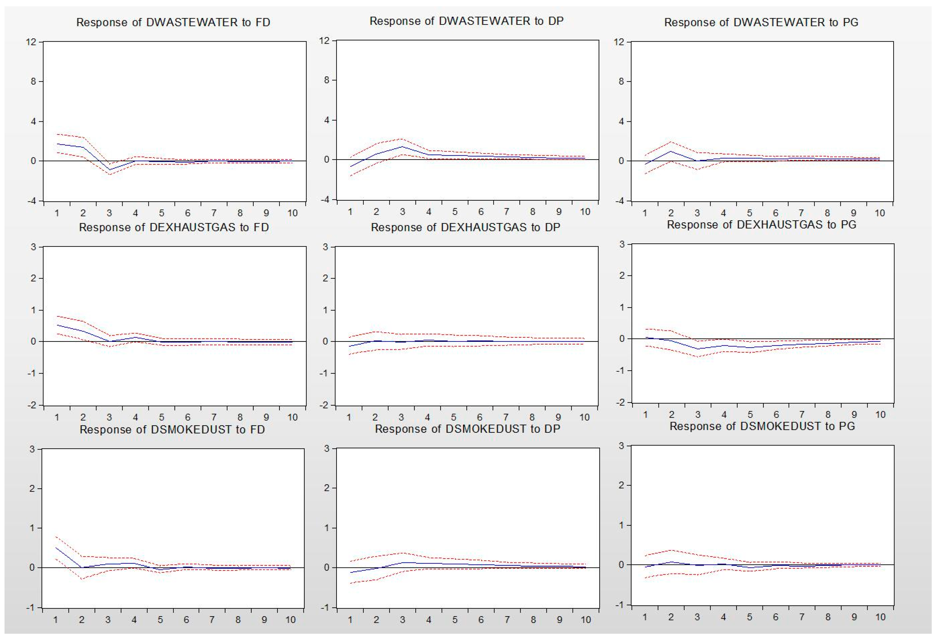
Based on the constructed PVAR model, the impulse response function of each pollution index’s response to changes in fiscal decentralization, debt pressure, and poverty governance impact was plotted. The impulse response function can fully demonstrate the entire process of one variable affecting another. Therefore, the impulse response function provides us with an effective tool for observing the full impact of various influencing factors at the system level on environmental pollution. This paper uses Cholesky decomposition technology to draw the impulse response function based on the PVAR model estimation results shown in Figure 1.

From Figure 1, it can be seen that the impact of a positive standard deviation of one unit of fiscal autonomy brings a significant drop in dwastewater, dexhaustgas, and dsmokedust. Dexhaustgas and dsmokedust reached the lowest point in the third period and remained stable thereafter. This shows that the improvement of FD has effectively curbed the degree of environmental pollution and eased the pressure on the environment. With the official performance appraisal gradually changing the status quo of the GDP-only theory, the country’s transformation of the economic development mode, and vigorously promoting the policy orientation of green development, the expansion of the local government’s financial power makes local governments have more funds to invest in the regional environment to improve the mode of economic development. On top of that, it brings about a reduction in the degree of pollutant emissions. Hypothesis 1 is verified.

The impact of one unit of positive standard deviation of DP brought a rise in the dwastewater, dexhaustgas, and dsmokedust. Among them, DP had the most obvious effect on the elevation of dwastewater, followed by dexhaustgas, and it had the weakest effect on dsmokedust. However, overall, with the expansion of DP, the total discharge of pollutants increased. This shows that under the pressure of very large debt-servicing and repayment, local governments have to pay off debts in order to circumvent the crisis of government credibility, reducing environmental barriers to attract investments and obtain debt-recovery funds at the cost of polluting the environment. Hypothesis 2 is verified.

After being affected by the positive standard deviation of one unit of PG, dwastewater starts from 0, rises to the highest point in the second period, returns to 0 in the third period, and then remains at the 0 point level, indicating that PG’s increase caused short-term fluctuations in dwastewater, but it did not cause the actual rise and fall of dwastewater. At the same time, dexhaustgas dropped from 0 to the lowest point in the third period, then slowly returned to 0, indicating that the increase in PG brought about a reduction in dexhaustgas in the short term. However, in the long term, it did not cause significant changes in dexhaustgas. Finally, dsmokedust stayed at 0 for a long time, indicating that the increase in PG did not affect the changes in dsmokedust. Summarizing the above three impulse response function diagrams, the influence of the increase of PG on different pollutants is not the same and the number of pollutants did not significantly increase. Therefore, there is no “PPE circle” in China. Hypothesis 3a has not been verified.

5.4. Construction and Inspection of a Long-Term Panel Regression Model

The impulse response function can only show the impact of one variable after a positive change in another variable. That is to say, when studying the relationship between the poverty population and environmental pollution, the impulse response function can only show the increase of the poor population to the environment. The impact does not explain the effect of the reduction of poverty on environmental pollution. Therefore, we cannot just rely on the impulse response function to study whether the current poverty reduction in China will have a negative impact on the environment. Based on this, in order to test hypothesizes again, especially to test Hypothesis 3b, we introduced panel regression Models (2)–(4).

In the panel regression model, FD, DP, and PG were used as explanatory variables, and wastewater, exhaustgas, and smokedust were used as explained variables, respectively. Referring to the existing literature, we introduced RC, ED, and EC as control variables. RC is used to demonstrate the impact of changes in the local government financial power on the environmental pollution under regional competition, ED is used to illustrate the extent of economic development on the environment, and EC is used to illustrate that the increase in energy consumption will lead to an increase in pollutant emissions, which will lead to environmental damage.

In order to solve the possible endogenous problems between explanatory variables and explained variables, we first used the Toda-Yamamoto Granger causality test to explore the mutual predictive relationship between variables. If there is a strong mutual predictive relationship between explanatory variables and explained variables, then we need to solve the endogeneity problem first. In the discussion of the previous section, the three variables of EP (wastewater, exhausttgas, and smokedust) are I (1) (first-order single integer variables), and FD, DP, and PG are all sequences of the original order. Therefore, we cannot use the traditional Granger causality test to explore the prediction relationship between them. In fact, same order mono is a necessary basis for cointegration between variables. However, each variable in this paper no longer satisfies this condition. Therefore, the traditional Granger causality test based on the original sequence’s stability or the existence of a cointegration relationship loses its application foundation. The advantage of this status quo is that the probability of a “pseudo-regression” in panel regression is greatly reduced. We can use the Toda-Yamamoto Granger causality test that does not depend on cointegration to explore the mutual predictive relationship between variables. This method was proposed by Toda and Yamamoto in 1995. First, determine dmax (the highest possible single integer order) in the variable, then establish an extended “p+dmax” order VAR model. With the modified Wald test, it is determined whether a variable has a Granger significance causality for other variables by examining whether the coefficient of the p-order lag term is significantly equal to zero at the same time. Obviously, the highest single integer order in this paper is 1, and the optimal lag period for the VAR model determined by the AIC criterion is 3. Therefore, the VAR (3 + 1) model was established. The final results of Toda-Yamamoto Granger causality test are shown in

Table 7. Toda-Yamamoto Granger causality test results.

		Results
		Wastewater	Exhaustgas	Smokedust	FD	DP	PG
Causes	wastewater				6.3488 *	0.3792	0.6609
	exhaustgas				21.1912 ***	11.2597 ***	8.7010 **
	smokedust				5.5083	3.0061	2.0015
	FD	29.7346 ***	18.0066 ***	17.9250 ***
	DP	1.6544	34.1334 ***	34.9147 ***
	PG	0.4143	31.3163 ***	30.4065 ***

* p < 0.1; ** p < 0.05; *** p < 0.01. same as below.

.

As can be seen from Table 7, when FD, DP, and PG are used as Granger causes, except for DP and PG is not Granger causality for wastewater, other results show that the three variables (FD, DP, PG) are all significant Granger causes for EP variables (wastewater, exhaustgas, smokedust). On the contrary, when the EP’s three variables (wastewater, exhaustgas, smokedust) are the causes, except that exhaustgas is the Granger cause of FD and DP, other results show that EP variables are not Granger causes of FD, DP, and PG. Overall, the endogenous problems in panel regression models are not serious. However, in order to more completely mitigate the adverse consequences of the endogeneity problems in the model, we used the lag one-phase independent variable and the current dependent variable in the subsequent regression.

In Models (2)–(4), the concomitant probabilities of the test statistics for each model passed the hausman test were less than 0.05, so we decided to establish fixed effect models. This part uses the panel data of 30 provinces from 2001 to 2016. In order to eliminate the influence of heteroscedasticity, DP, RC, ED, and EC were taken logarithmically. The results of the regression are shown in

Table 8. The long-term panel regression results.

Variables	Model (2)	Model (3)	Model (4)
	Wastewater	Exhaustgas	Smokedust
FD	$-2.2212{ }^{***}$	$0.5252{ }^{ *}$	$-0.9532{ }^{***}$
	(−3.7721)	(1.6707)	(−3.9491)
DP	−0.6316	$0.7017{ }^{**}$	$-0.1290$
	(−0.9935)	(2.0675)	(−0.4951)
PG	$-0.1116{ }^{***}$	$0.0583{ }^{***}$	$-{0.0279}^{ ***}$
	(−4.6431)	(4.5467)	(−2.8320)
RC	$-1.1869{ }^{***}$	$-{1.2716}^{ ***}$	$-0.3385{ }^{***}$
	(−2.8871)	(−5.7942)	(−2.0085)
ED	$26.2068{ }^{***}$	$-12.4236{ }^{***}$	$-7.8311{ }^{***}$
	(15.8940)	(−14.1140)	(−11.5866)
EC	$-2.5203{ }^{***}$	${8.2169}^{ ***}$	$5.0407{ }^{***}$
	(−4.0178)	(24.5377)	(19.6040)
R2	0.5425	0.8593	0.8491

* p < 0.1; ** p < 0.05; *** p < 0.01. same as below.

.

Except for Model (3), FD has a significant negative correlation with both wastewater and smokedust, indicating that with the increase of FD, the government has more energy and funds to focus on environmental governance, resulting in an improved environment. This is consistent with the conclusions obtained in the impulse response function.

The results of DP show differences in the three models. In Models (2) and (4), the relationship between DP and wastewater, exhaustgas, and smokedust was not tested. Model (3) showed that DP and exhaustgas were significantly positively correlated. The reason for this phenomenon may be that the relationship between DP and exhaustgas may not be linear and that the coefficients of regression equation reflect only a local dynamic relationship, so a simple linear regression equation cannot show the complexity between the two. In contrast, the impulse response function captures the overall complex and dynamic relationships between variables and, thus, can demonstrate the overall change in environmental pollution as the poverty population changes.

From Model (2), it can be seen that PG and wastewater are significantly negatively correlated. Considering that, since 2001, the number of people in poverty in China has been on a downward trend, and poverty governance has continued to progress, there is no increase in poverty. Therefore, the regression results of Model (2) show that with the decrease of PG, water continuously increases and water pollution is aggravated. The regression results of Model (4) showed that there was a significant negative correlation between PG and smokedust, indicating that as PG decreased, smokedust increased, causing environmental pollution. However, we can also see that in Model (3), with exhaustgas as the explained variable, there is a significant positive correlation between PG and exhaustgas, indicating that with the decrease of PG, exhaustgas is significantly reduced and that the air pollution situation improves. Based on the above regression results, Models (2) and (4) accept Hypothesis 3b. It is believed that the reduction of the poverty population is at the cost of environmental pollution. However, Model (3) rejects Hypothesis 3b and believes that China’s poverty governance has not caused an increase in atmospheric pollutant emissions for a long time. The reason that this paper uses “exhaustgas” (industrial sulfur dioxide emissions) as a variable to quantify the degree of environmental pollution is special. Industrial sulfur dioxide is one of the major pollutants in air pollution and it is also the culprit of the current urban haze phenomenon. For a long time, the air quality of major cities has been unsatisfactory and has become an important factor affecting the daily health of urban residents, especially the haze problem in large cities, such as Beijing. Under the pressure of strong public opinion, major cities have formulated relevant policies and measures to carry out haze governance. More than 20 provincial governments have all introduced and successively implemented relevant measures for controlling air pollution, and the air pollutant emissions have been initially controlled throughout the country. Air pollution control has become a pioneering area in the entire field of environmental governance and has achieved certain results. Therefore, with strong policy guidance, exhaustgas, and PG have shown a significant positive relationship, revealing a clear downward trend between the two. Based on the above results, we can conclude that for a long time, the reduction of PG in China led to a significant increase in water and gas pollution, but in the area of air pollution control, gas pollution did not conflict with PG. On the whole, China has long achieved the goal of reducing poverty at the cost of the environment.

5.5. The Relationship between Poverty Governance and Environmental Pollution in the New Period

It is worth noting that China’s proposal for a 2020 victory to eradicate poverty and further implement the green development strategy is something that has happened since 2012. Therefore, when we study the relationship between poverty governance and environmental pollution under policy pressures, the data since 2012 is a more accurate research window. Therefore, we have selected the data from 2012 to 2016 in this part to conduct further research on environmental pollution caused by fiscal stress and poverty governance. Based on this, in order to test hypotheses again, especially to test hypothesis 3b, we introduced panel regression Models (5)–(7). The concomitant probabilities of the test statistics for each model that passed the Hausman test were less than 0.05, so we decided to establish fixed effect models to test the effect of FD, DP, and PG on EP in 2012–2016. The model regression results with EP (wastewater, exhaustgas, and smokedust) as explained variables are shown in

Table 9. The new period panel regression results.

Variables	Model (5)	Model (6)	Model (7)
	Wastewater	Exhaustgas	Smokedust
FD	−0.4146	−$4.0299{ }^{***}$	−$2.0405{ }^{***}$
	(0.7366)	(6.1335)	(5.6653)
DP	0.1084	0.3571	$0.2970{ }^{*}$
	(0.5859)	(1.3333)	(1.7485)
PG	0.0193	0.0145	0.0049
	(1.5287)	(1.2539)	(0.8652)
RC	0.1441	${3.1245}^{ ***}$	0.9864
	(0.1625)	(3.4952)	(1.4867)
ED	$7.5524{ }^{***}$	$-17.1190{ }^{***}$	$2.6331{ }^{**}$
	(4.6036)	(−12.0991)	(2.6142)
EC	−1.1743	$-{3.6380}^{ ***}$	$-2.1221{ }^{***}$
	(−1.2900)	(−3.5592)	(−2.8985)
R2	0.9705	0.9117	0.9300

* p < 0.1; ** p < 0.05; *** p < 0.01. same as below.

.

FD is negatively related to EP. In Models (6) and (7), there was a significant negative correlation between FD and exhaustgas or smokedust. In Model (5), the relationship between FD and EP is not significant, but the coefficient is positive. It shows that, since 2012, the expansion of fiscal power in various regions has brought about a reduction in the emissions of various environmental pollutants. This is consistent with the conclusions reached earlier and, once again, Hypothesis 1 is confirmed.

In Models (5)–(7), DP and EP were positively correlated, in which Models (5) and (6) were not significant and Model (7) was significantly positively correlated. Again, verifying Hypothesis 2.

Models (5)–(7) did not test the significant correlation between PG and EP, but from the regression coefficient point of view, the regression coefficients of PG in the three models are all positive. This result indicates that the PG decreased with the reduction of EP. Basically verifying H3b again. This result can illustrate two issues. First, China has adopted a policy of transforming the mode of economic development, implementing the policy of green development, and reducing economic and social development at the cost of the environment. Over the past few years, poverty alleviation and fighting against economic development have become less dependent on environmental destruction and this has brought about a non-significant regression coefficient. Second, environmental protection and economic development are not fundamentally antagonistic. We can achieve environmental protection in the process of promoting economic development, and we can even exchange economic development from environmental protection. Under the guidance of green development, poverty governance is gradually drawing on nutrients from environmental protection to achieve a mutually beneficial win-win situation between environmental protection and poverty governance, thus, bringing about a positive regression coefficient. Based on the above results, it can be proved that in recent years, China’s strategy of comprehensively eradicating poverty and promoting the transformation of economic development methods and realizing green development has not produced conflicting phenomena. In the process of poverty reduction by local governments, there was no environmental sacrifice. In exchange for the effect of reducing poverty, at this stage, especially in recent years, there has been no “environmental trap” in China.

In summary, wastewater, exhaustgas, and smokedust are used as surrogate variables of EP to measure their response to FD, DP, and PG, respectively, and a relatively consistent conclusion is drawn. This shows that this study has robustness.

6. Conclusions

This article summarizes the factors affecting EP at the institution level as FD, DP, and PG. By plotting the impulse response function map and building a panel regression model under the PVAR model, the effects of FD, DP, and PG on EP were studied at the institutional level. Through empirical research, the main conclusions are as follows:

(1)

The improvement of FD will help reduce EP, and hypothesis 1 is verified, which shows that the expansion of local financial power will help local governments increase their environmental input and ease the current status of EP.

(2)

DP has increased EP, and hypothesis 2 is verified, which shows that the expansion of local government debt has caused local governments to face enormous pressures on debt and interest payments. In order to avoid the government’s credibility crisis, local governments have sacrificed the environment in exchange for debt income.

(3)

The growth of PG has not caused the deterioration of EP. There is no “PPE trap” problem in China. Hypothesis 3a is not verified.

(4)

For a long time, China’s environment has indeed suffered in order to achieve the goal of reducing poverty, which is mainly related to China’s early national economic development as the center and the neglect of environmental protection. Hypothesis 3b is verified. However, in recent years, the central government has resolutely resolved to implement the concept of green development by changing the mode of economic development, not only to reduce the damage to the environment caused by economic development, but also to absorb the nutrients that promote economic development from environmental protection undertakings. In the past five years, China’s poverty reduction efforts have not brought environmental pollution. Instead, it has brought about a reduction in the emission of all types of pollutants. This shows that China’s policies of eradicating poverty and implementing the green development strategy by 2020 do not contradict each other. There is no “environmental trap” problem in China’s poverty governance.

Based on the above findings, this paper proposes the following policy recommendations:

(1)

Firstly, accelerating reforms of the fiscal and taxation institutions that give greater financial autonomy to local governments and, at the same time, radically change the assessment mechanism of GDP-only for officials to promote a new assessment mechanism should include environmental performance. In the process, local governments will be freed from the vicious circle of economic development and environmental pollution. They will have greater motivation and more funds to improve the ecological environment.

(2)

Secondly, local government should control the scale of debt, establish a sound early warning mechanism for local government debt risks, control the scale of local government debt within a reasonable range, ensure that local governments have a stronger ability to pay off debts and reduce debt, and reduce the pressure on debt to prevent local governments from furthering environment pollution.

(3)

Third, poverty governance and transformation of economic development methods must be implemented in a green economy. It is necessary to guard against the adverse effects of poverty reduction and poverty eradication on the environment and to prevent damages to people in poverty in transforming economic development patterns.

(4)

Fourth, institutions need to play an active role in environmental governance. On the one hand, we must strengthen the supervision of the market and severely crack down on environmental pollution in economic development. On the other hand, we must examine institution-level design deficiencies and adjust the institution deficiencies in a timely manner to eliminate the potential damage to the ecological environment at the institution level, to aggravate the potential factors of environmental pollution, and to promote the healthy economic development and the continuous improvement of the ecological environment.

Of course, there are two caveats related to this study that should be raised at this point:

(1)

Firstly, linear panel regression finds it difficult to reflect the nonlinear relationship between variables, so, in the panel regression, the impact of DP on EP does not reach a consistent conclusion, although in the impulse response function, a DP-positive impulse brings about an increase in EP, but the impulse response function reflects only a long-term and macro relationship which is relatively insufficient for portion and short-term reflections. Therefore, the study on the complex nonlinear relationship of DP affecting EP is relatively insufficient.

(2)

Secondly, we do not test the existence of an “environmental Kuznets curve” in China. The “Environment Kuznets Curve” believes that before a country’s economic development reaches a certain level, the economic development will inevitably depend on environmental destruction and resource development and utilization, and that the resulting environmental pollution will be unavoidable. Only reaching a certain level of economic development will contribute to environmental protection, which is what we commonly call the “pollution first, then governance” development path. In China, to verify the existence of the “Environment Kuznets Curve”, two conditions must be met. The first is the selection of the pole of the curve, that is, whether China has reached the extreme point of the “Environment Kuznets Curve”. This is not conclusive in the academic world. Second, China needs a long enough development time to serve as a research window for the “Environment Kuznets Curve”.

Based on this, there are at least three future research prospects of this paper. Firstly, to find a more appropriate method to study the nonlinear relationship between DP and EP, to explore the notion that DP is conducive to environmental protection, and to make full use of this short-term, partial relationship to serve environmental protection. Secondly, using international data as a research sample, to determine the extreme points of the “Environment Kuznets Curve” as a reference for the “Environment Kuznets Curve” study in China, and to expand the research timeframe and sample size to explore whether China really exists in an “Environmental Kuznets Curve”. Thirdly, environmental non-governmental organizations (ENGOs) play an increasingly important role in the process of environmental governance, especially in some developing countries, such as China [76]; therefore, future environmental governance should take into account the impact of ENGOs.

References

1. Tian, S.; Dong, Y.; Xu, W. Environmental fiscal expenditures, government environmental preferences, and policy effects. Explor. Econ. Issues 2016, 6, 14–21. [Google Scholar] [CrossRef]
2. Environmental Performance Index 2014. Available online: https://epi.envirocenter.yale.edu/ (accessed on 5 may 2018).
3. The World Air Quality Index 2014. Available online: https://www.drmj.org/the-world-air-aap-2016-who.html (accessed on 5 May 2018).
4. Pigou, A.C. The Econ. of Welfare; Macmillan: London, UK, 1920. [Google Scholar]
5. Coase, R.H. The Problem of Social Cost; The University of Chicago Press: Chicago, IL, USA, 1960; Volume 3, pp. 1–44. [Google Scholar]
6. Coase, R.H. The federal communications commission. J. Law Econ. 1959, 2, 1–40. [Google Scholar] [CrossRef]
7. Guo, Z.; Zheng, Z. Fiscal Decentralization, Promotional Incentives, and Environmental Pollution: An Analysis Based on Provincial Panel Data from 1997 to 2010. J. Southwest Univ. Natl. Humanit. Soc. Sci. 2013, 3, 103–107. [Google Scholar]
8. Tian, X.; Xia, S. The research on the impact of local government debt risk. J. Shanxi Univ. Financ. Econ. 2017, 39, 26–38. [Google Scholar] [CrossRef]
9. Available online: http://www.xinhuanet.com/politics/2015-11/28/c_1117292150.htm (accessed on 5 May 2018).
10. Sun, Y. The government’s poverty governance capacity and its promotion path. Receigar Dev. 2015, 3, 31–34. [Google Scholar] [CrossRef]
11. Jacobsen, G.; Kotchen, M.; Vandenbergh, M. The behavioral response to voluntary provision of an environmental public good: Evidence from residential electricity demand. Eur. Econ. Rev. 2012, 59, 946–960. [Google Scholar] [CrossRef]
12. He, Q. Fiscal decentralization and environmental pollution: Evidence from Chinese panel data. China Econ. Rev. 2015, 36, 86–100. [Google Scholar] [CrossRef]
13. Li, G.; Han, M. Fiscal decentralization, spatial spillover and China’s urban Haze pollution: Mechanism and evidences. Cont. Financ. Econ. 2015, 6, 26–34. [Google Scholar] [CrossRef]
14. Malueg, D.A.; Yates, A.J. Strategic behavior, private information, and decentralization in the European Union emissions trading system. Environ. Resour. Econ. 2009, 43, 413–432. [Google Scholar] [CrossRef]
15. Böhringer, C.; Rivers, N.; Yonezawa, H. Vertical fiscal externalities and the environment. J. Environ. Econ. Manag. 2016, 77, 51–74. [Google Scholar] [CrossRef] [Green Version]
16. Banzhaf, H.S. Designing economic instruments for the environment in a decentralized fiscal system. J. Econ. Surv. 2012, 26, 177–202. [Google Scholar] [CrossRef]
17. McKinstry, R.B.; Rose, A.; Ripp, C. Incentive-based approaches to greenhouse gas mitigation in Pennsylvania: Protecting the environment and promoting fiscal reform. Widen. Law J. 2004, 14, 205–267. [Google Scholar]
18. López, R. Fiscal spending and the environment: Theory and empirics. J. Environ. Econ. Manag. 2011, 62, 180–198. [Google Scholar] [CrossRef]
19. Que, W.; Zhang, Y.; Liu, S.; Yang, C. The spatial effect of fiscal decentralization and factor market segmentation on environmental pollution. J. Clean. Prod. 2018, 184, 402–413. [Google Scholar] [CrossRef]
20. Spencer, B.H.; Chupp, B. Andrew. Fiscal federalism and interjurisdictional externalities: New results and an application to US air pollution. J. Public Econ. 2012, 96, 449–464. [Google Scholar] [CrossRef]
21. Gupta, M.R. Fiscal policies, environmental pollution and economic growth. Econ. Model. 2009, 26, 1018–1028. [Google Scholar] [CrossRef]
22. Herber, B.P. Pigovian taxation at the supranational level: Fiscal provisions of the international oil pollution compensation fund. J. Environ. Dev. 1997, 6, 110–122. [Google Scholar] [CrossRef]
23. Sigman, H. Decentralization and Environmental Quality: An International Analysis of Water Pollution, NBER Working Paper. 2007. Available online: http://www.nber.org/papers/w13098 (accessed on 5 May 2018).
24. Holmstrom, M. Multitask Principal—Agent Analyses: Incentive Contracts, Asset Ownership, and job Design. J. Law Econ. Organ. 1991, 1, 24–52. [Google Scholar] [CrossRef]
25. Yang, R.; Zhang, Q.; Zhou, Y. Fiscal Decentralization, Public Preferences, and Environmental Pollution—Evidence from Chinese Provincial Panel Data; Working Paper of Renmin University of China; Renmin University: Beijing, China, 2007. [Google Scholar]
26. Liu, Q. Fiscal decentralization, governmental incentives and environmental pollution abatement. Econ. Surv. 2013, 2, 127–132. [Google Scholar] [CrossRef]
27. Wu, J.; Wan, G. The transmission mechanism and effect of fiscal decentralization on environmental pollution: An ampirical study based on municipal panel data. J. Guangxi Univ. Financ. Econ. 2016, 6, 37–45. [Google Scholar]
28. Yan, W.; Zhong, M. Can Chinese-style fiscal decentralization increase envirenmental pollution. Collect. Essays Financ. Econ. 2012, 3, 32–37. [Google Scholar] [CrossRef]
29. Xue, G.; Pang, X. An empirical analysis on the impact of fiscal decentralization on environmental pollution in China. China Popul. Resour. Environ. 2012, 22, 77–83. [Google Scholar]
30. Tan, Z.; Zhang, Y. An empirical research on the relation between fiscal decentralization and environmental pollution. China Popul. Resour. Environ. 2015, 25, 110–117. [Google Scholar]
31. Li, M. Fiscal Decentralization and Environmental Pollution—Revision of the Environmental Kuznets Hypothesis. Econ. Rev. 2009, 5, 54–59. [Google Scholar] [CrossRef]
32. Deng, Y. Fiscal expenditure structure and environmental pollution: Empirical research based on the panel threshold model. Meteorol. Environ. Res. 2018, 9, 32–37. [Google Scholar] [CrossRef]
33. Liu, J.; Chen, X.; Wu, J. Fiscal Decentralization, Local Government Competition, and Environmental Pollution—Analysis of Heterogeneity and Dynamic Effects Based on 272 Urban Data. Financ. Res. 2015, 9, 36–43. [Google Scholar] [CrossRef]
34. Kim, D.-H.; Suan, Y.-B.; Lin, S.-C.; Hsieh, J. Government size, government debt and globalization. Appl. Econ. 2018, 50, 2792–2803. [Google Scholar] [CrossRef]
35. Andolfatto, D.; Martin, F.M. Monetary policy and liquid government debt. J. Econ. Dyn. Control 2018, 89, 183–199. [Google Scholar] [CrossRef]
36. Faulk, D.; Killian, L. Special districts and local government debt: An analysis of ‘Old Northwest Territory’ States. Public Budg. Financ. 2017, 37, 112–134. [Google Scholar] [CrossRef]
37. Liu, C.; Moldogaziev, T.T.; Mikesell, J.L. Corruption and state and local government debt expansion. Public Adm. Rev. 2017, 77, 681–690. [Google Scholar] [CrossRef]
38. Cassou, S.; Shadmani, H.; Vazquez, J. Fiscal policy asymmetries and the sustainability of US government debt revisited. Empor. Econ. 2017, 53, 1193–1215. [Google Scholar] [CrossRef]
39. Lu, M.; Zhong, H. Eurozonization of the Chinese economy: How do intergovernmental transfers affect local government debt in China. Asian Econ. Pap. 2018, 17, 1–18. [Google Scholar] [CrossRef]
40. Li, S.; Liang, Y. Competition model and the change of local governments’ behavior—And governance of China’s local government debt. Chin. Econ. 2016, 49, 199–212. [Google Scholar] [CrossRef]
41. Kopczewska, K.; Kudla, J.; Walczyk, K.; Kruszewski, R.; Kocia, A. Spillover effects of taxes on government debt: A spatial panel approach. Policy Stud. 2016, 37, 274–293. [Google Scholar] [CrossRef]
42. Hu, Y.; Gu, Y. Local government debt and the economic growth. Audit. Res. 2016, 5, 104–112. [Google Scholar]
43. Xia, S. The Study of Long-term and Short-term Dynamics of Government Debt, Fiscal Deficit, and Economic Growth during the Transitional Period. Macroeconomics 2017, 3, 68–77. [Google Scholar] [CrossRef]
44. Salotti, S.; Trecroci, C. The impact of government debt, expenditure and taxes on aggregate investment and productivity growth. Economica 2016, 83, 356–384. [Google Scholar] [CrossRef]
45. Cheng, Y.; Gong, L. Government debt and economic growth. J. Quant. Tech. Econ. 2014, 12, 22–37. [Google Scholar]
46. Coupet, E., Jr. Government debt and economic growth: Another Neoclassical growth approach. J. Appl. Econ. Bus. Res. 2017, 7, 172–193. [Google Scholar]
47. Diao, W. A research on the moderate scale of China’s local government debt in the perspective of economic growth: Using the provicial data. Econ. Probl. 2016, 3, 50–54. [Google Scholar] [CrossRef]
48. Chen, Z.; Wu, G. Does local government debt promote regional economic growth? Mod. Financ. Econ. 2018, 4, 48–60. [Google Scholar] [CrossRef]
49. Chen, C.; Yao, S.; Hu, P.; Lin, Y. Optimal government investment and public debt in an economic growth model. China Econ. Rev. 2017, 45, 257–278. [Google Scholar] [CrossRef]
50. Lin, F.; Zhao, Y. Does government debt affect multiplier effect of fiscal expenditure? A cross-country analysis. J. Financ. Econ. 2018, 2, 58–74. [Google Scholar] [CrossRef]
51. Winter, C. The impact of government debt on the long-run natural real interest rate—A quantitative evaluation. Appl. Econ. Lett. 2017, 24, 1429–1434. [Google Scholar] [CrossRef]
52. Zhang, Y.; Cheng, Y.; Hu, Q. Quantitive analysis of local government debt default’s influence on China’s macrofunds flow: On input-output macro flows of funds method. Financ. Trade Res. 2018, 3, 1–10. [Google Scholar] [CrossRef]
53. Mao, R.; Liu, N.; Liu, R. The expansion of local government debt and the mechanism of systemic financial risk triggering. China Ind. Econ. 2018, 4, 19–38. [Google Scholar] [CrossRef]
54. Wang, B.; Liu, W. Local government debt expansion and livelihood development. Res. Financ. Econ. Issues 2018, 1, 85–90. [Google Scholar]
55. Chen, H.; Yang, Q. Research on the Relationship between Government Debt and Private Investment—Comparison between OECD Countries and China. Stud. Int. Financ. 2017, 12, 17–24. [Google Scholar] [CrossRef]
56. Xian, G.; Leng, Y. Local government debt, financial development and FDI: An empirical research. Nankai Econ. Stud. 2016, 3, 52–74. [Google Scholar] [CrossRef]
57. Ouedraogo, B. Household energy preferenceces for cooking in urban Ouagadougou, Burkina Faso. Energy Policy 2006, 34, 3787–3795. [Google Scholar] [CrossRef]
58. Abhilash, R.C. Nandita Singh. Pesticide use and application: An Indian scenario. J. Hazard. Mater. 2009, 165, 1–12. [Google Scholar] [CrossRef] [PubMed]
59. Swanson, K.E.; Kuhn, R.G.; Xu, W. Environmental policy implementation in rural China: A case study of Yuhang, Zhejiang. Environ. Manag. 2001, 27, 481–491. [Google Scholar] [CrossRef]
60. Zhang, W.; Yuan, J.; Luo, X. Economic development gap, enforcement of environmental regulation and environmental pollution insurance system design. J. Financ. Econ. 2015, 30, 119–128. [Google Scholar]
61. Jiang, X.; Yan, T. An EKC-based analysis of coordinated economic development and environmental protection in poverty-stricken areas based: A case study of zhaotong, yunnan province. Comp. Econ. Soc. Syst. 2016, 3, 31–39. [Google Scholar]
62. Grossman, G.M.; Krueger, A.B. Economic growth and the environmental. Q. J. Econ. 1995, 110, 353–377. [Google Scholar] [CrossRef]
63. Li, Z. On poverty and environmental circulation in developing countries. Econ. Rev. 2007, 6, 83–92. [Google Scholar]
64. Lu, C. Research on poverty in developing countries—Based on the perspective of environment and population. Explor. Econ. Issues 2013, 12, 144–148. [Google Scholar]
65. Cao, S. Coupling between ecological vulnerability and economic poverty in contiguous destitue areas in China. Chin. J. Appl. Ecol. 2016, 27, 2614–2622. [Google Scholar]
66. Oates, W. A reconsideration of environmental federalism. Discuss. Pap. 2001, 56, 171–197. [Google Scholar]
67. Moons, E.; Bert, S.; Stef, P.; Hermy, M. Optimal location of new forests in a suburban region. J. For. Econ. 2008, 14, 5–27. [Google Scholar] [CrossRef]
68. Steele, S.R. Expanding the solution set: Organization economics and agri-environmental policy. Ecol. Econ. 2009, 69, 398–405. [Google Scholar] [CrossRef]
69. Grant, J.P. The State of the World’Children; UNICEF/Oxford University Press: New York, NY, USA, 1994. [Google Scholar]
70. Li, Y. Poor Coordination of Economic and Economic Growth. Chin. Soc. Sci. 1991, 4, 199–210. [Google Scholar]
71. Fromont, P.; Myrdal, G. Rich lands and poor: The road to the world prosperity. Am. Sociol. Rev. 1960, 11, 146–147. [Google Scholar] [CrossRef]
72. Kuznets, S. Economic growth and income inequality. Am. Econ. Rev. 1955, 45, 1–28. [Google Scholar]
73. Stern, D.I. Progress on the Environmental Kuznets Curve? Working Papers in Ecological Economics; Cambridge University Press: Cambridge, UK, 1960. [Google Scholar]
74. Armeanu, D.; Vintilă, G.; Andrei, J.V.; Gherghina, Ş.C.; Drăgoi, M.C.; Teodor, C. Exploring the link between environmental pollution and economic growth in EU-28 countries: Is there an environmental Kuznets curve? PLoS ONE 2018, 13, e0195708. [Google Scholar] [CrossRef] [PubMed]
75. Chen, S.; Gao, L. Central Region Relations: Measurement of Fiscal Decentralization and Reassessment of Mechanisms. Manag. World 2012, 6, 43–59. [Google Scholar]
76. Li, G.; Qiao, H.; Shao, S.; Cao, J. Environmental non-governmental organizations and urban environmental governance: Evidence from China. J. Environ. Manag. 2018, 206, 1296–1307. [Google Scholar] [CrossRef] [PubMed]
Figure 1. The impulse response function diagram.
Sustainability 10 01834 g001