5.1. Reverse Competition
First, we investigate the transfer price, which determines how to divide the reverse channel. Second, we analyze the return rate, which can be viewed as the performance of reverse channel, meanwhile, we also focus on the optimal collective proportion between collective members in order to compare IPR with CPR. Moreover, the parameters are set as follows:
,
,
, and these values will apply throughout the numerical analysis. In
Figure 2,
Figure 3,
Figure 4,
Figure 5,
Figure 6,
Figure 7,
Figure 8,
Figure 9,
Figure 10 and
Figure 11,
.
5.1.1. Comparison of Transfer Price
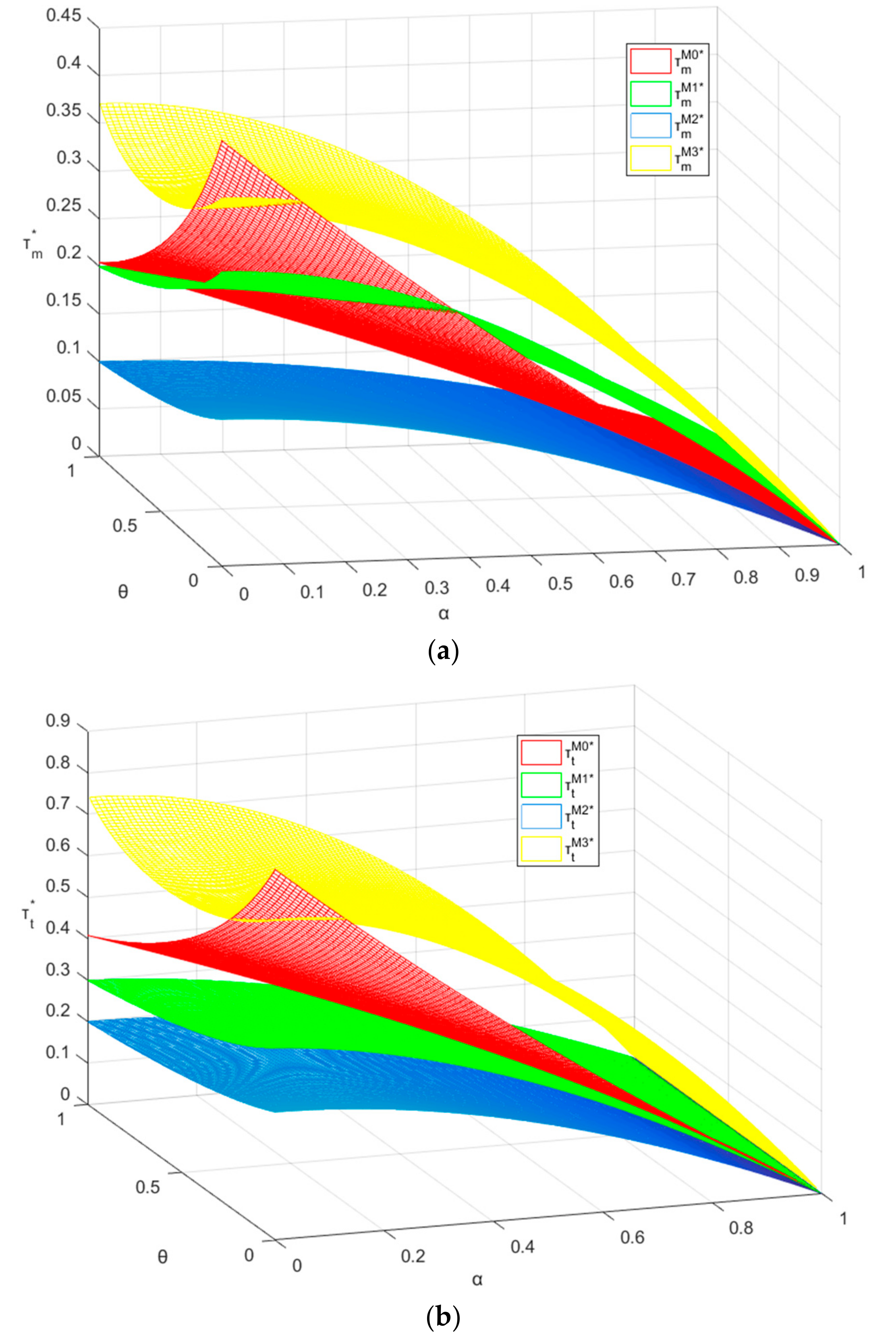
Proposition 1. The optimal transfer prices satisfy the following relationship: .
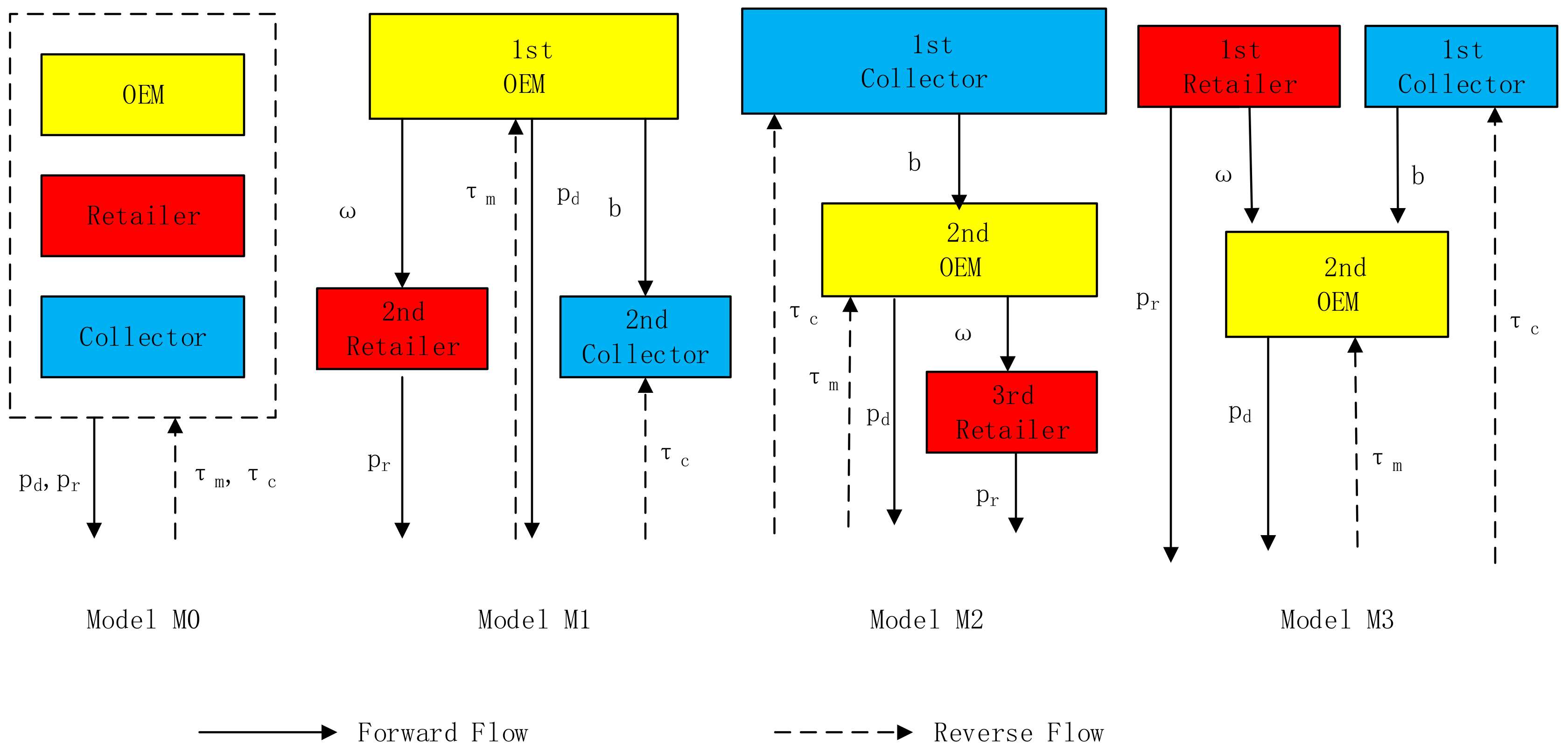
First, the optimal transfer price is lowest in M1 because it is offered by OEM, not the collector. Clearly, since the transfer price is lower than the cost saving from the remanufacturing, OEM could also benefit from the collector’s return rate. Also, if the transfer price is offered by the collector, the transfer price in M3 will be lower than in M2. When the collector leads the channel in M2, there are a first follower and a second follower in the three-echelon CLSC. When both the collector and retailer lead the channel in M3, there is only one follower. It implies that reverse competition is affected by the forward power configuration.
Second, transfer price plays a key role in the reverse channel. Total production cost will increase in the transfer price. Without restraints of the retailer in M3, the collector, as the single leader in M2, will offer the largest transfer price so that the total production cost is the largest. Meantime, OEM’s forward channel profit has also been extracted and forward channel is also distorted.
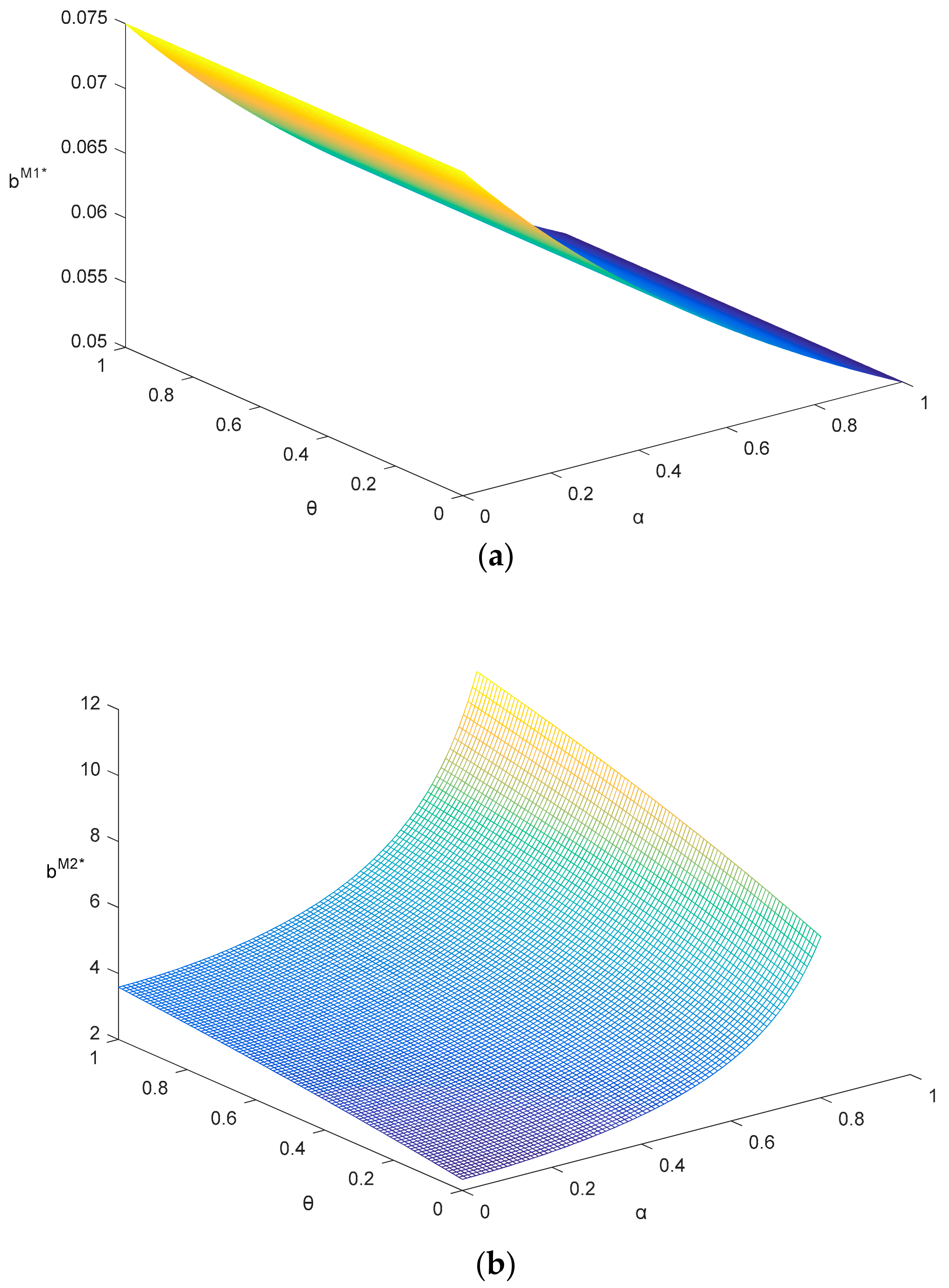
By
Figure 2, we can analyze the impact of dual competition intensities on the transfer price. If OEM leads the reverse channel in M1, transfer price decreases with
. Intuitively, as the competition increase, decreasing transfer price can not only strengthen their own competitiveness, but also beat the collector. However, if the collector is the leader, he will behave analogously as does OEM in
Figure 2b. Compared with transfer price irrelevant to
in M1,
will also increase in
. Since OEM compete in both channels, the collector raises the transfer price in order to beat OEM again as forward competition intensity increases. Then when
is larger, OEM will be exploit from both channel.
5.1.2. Collective Producer Responsibility (CPR) vs. Individual Producer Responsibility (IPR)
Compared with single reverse channel, reverse competition between the collector and OEM indicates double collection channel. From the perspective of extended producer responsibility (EPR), single channel can be regarded as individual producer responsibility (IPR) while double reverse channel implies collective producer responsibility (CPR). For IPR, EOL products could be collected by either OEM, or the collector. For CPR, it is essential to discuss the responsibility sharing between both members. Moreover, this part focuses on how the power configuration and competition intensity affect the responsibility sharing. Besides, we explain the advantage of CPR firstly.
On the one hand, from CLSC’s perspective, the profit under IPR and CPR is shown as follows:
Given the same condition, the profit of forward channel and the revenue of reverse channel under different policies are the same, except for reverse channel cost.
By the comparison, we can know if , i.e., no competition, CPR outperforms IPR. As goes up, the advantage of CPR decreases. If , the progress is even equal to .
On the other hand, from the perspective of OEM, his profit under CPR is composed of four parts, forward retail channel, forward direct channel, reverse collector’s channel, and reverse own channel, which is as follows:
Compared with IPR policy, OEM could benefit from his own reverse channel in addition under CPR. Likewise, as goes up, his profit of own reverse channel goes down, i.e., the advantage of CPR decreases.
Overall, if reverse competition is not fierce, CPR policy is preferred; otherwise, IPR policy is better. Intuitively, if both sides compete against each other, it is impossible to share the recycling market collectively. Next, Proposition 2 shows how the responsibility sharing is influenced by the power configuration and competition intensity.
Proposition 2. The optimal collective proportions are , where .
Proposition 2 indicates the optimal collective proportion only depends on the reverse power configuration. To be specific, the proportion is more than 1 and only depends on the reverse competition intensity if OEM leads the reverse channel. However, if the collector is the leader, the optimal proportion remains at 1 which is consistent with that in Model M0. That is, his return rate is equal to OEM’s. Namely, to optimize the performance of reverse channel, the perspective of the collector is consistent with that of CLSC, no matter who leads forward channel. Compared with the collector-led model, OEM’s return rate is higher if he is the leader. Because he can take control of the forward channel to affect the reverse channel. According to Proposition 2, we can compare the return rates. Before, we first introduce Corollary 1 to explain the relationship between return rate and sale quantities.
5.1.3. Comparison of Return Rate
Corollary 1. Return rate is increasing in the total quantities.
Return rate includes OEM’s return rate, collector’s return rate and total return rate. By Corollary 1, all kinds of return rates are all increasing in the total quantities. Since the reverse channel is determined by the return rate, Corollary 1 implies the reverse channel depends on the forward channel. And the larger forward channel leads to the larger reverse channel.
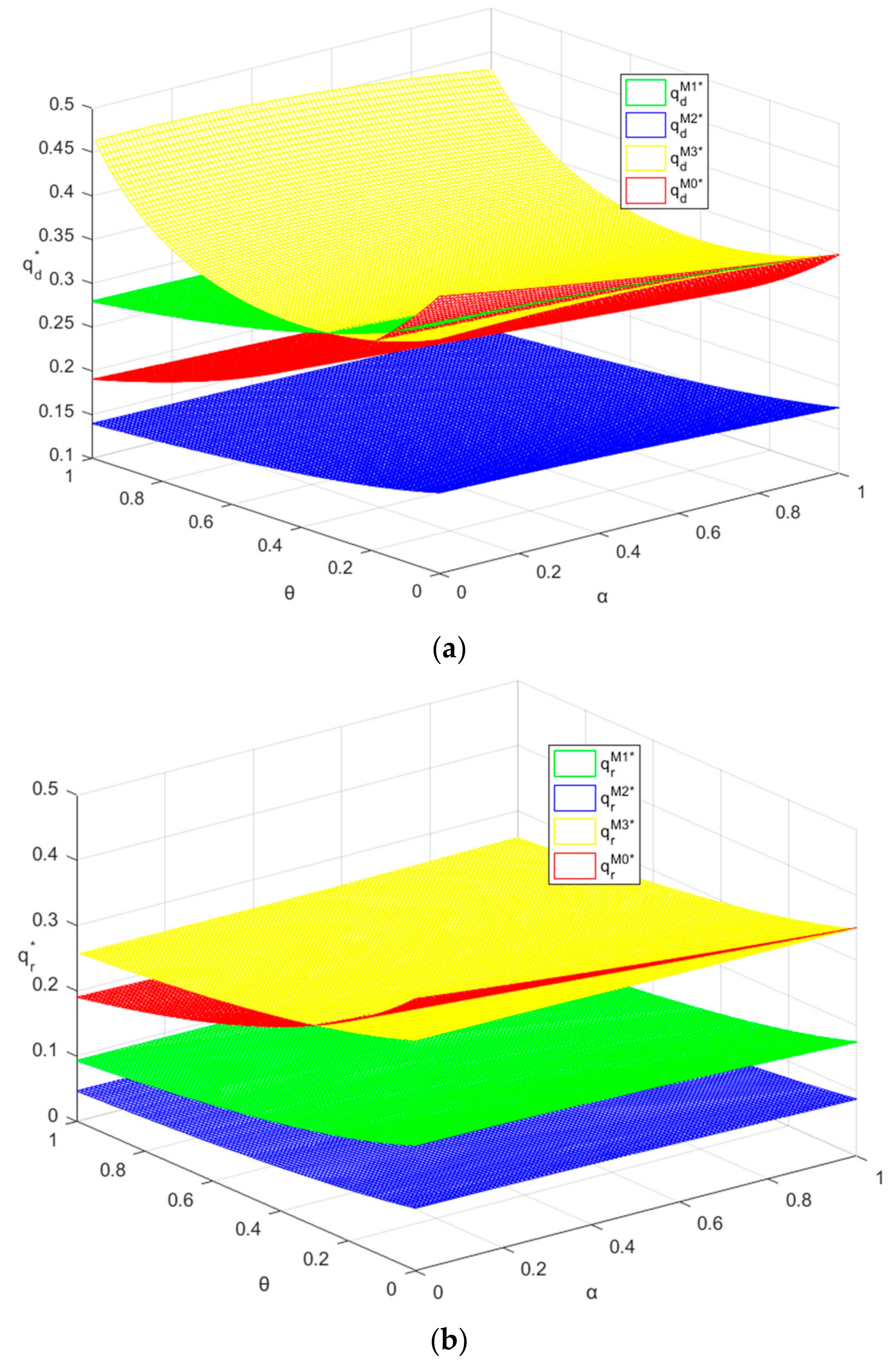
Proposition 3. (i) The optimal collector’s return rates satisfy . (ii) The optimal OEM’s return rates are related as follows:. If and only if and are larger,;if and only if and are smaller,.(iii) The optimal total return rates are related as follows:.
Proposition 3 shows the relationships of return rate between different models. Intuitively, is the smallest if the leader is OEM. Otherwise, the optimal collective propositions in other three models are all 1:1. Namely, the comparison of the collector’s return rate is also consistent with that of OEM’s. One of the decentralized models outperforms the centralized model in the return rate, while the other one underperforms. Combined with Proposition 1, if the collector is the unique leader in CLSC, his main means for raising his profit is to increase the transfer price. However, if the collector has to share the leadership with the retailer in M3, rising up the transfer price might be restrained by the behavior of the retailer. Then improving the performance of reverse channel is also significant for the collector. Hence, the collector’s return rate is highest in M3. This indicates all the aspects of reverse channel are influenced by the power positioning in the forward channel.
By Proposition 3(ii), the relationship between
is consistent with 3(i), but the ranking of
is influenced by the dual competition intensities. First, from the perspective of OEM, he can benefit from his own return rate. When OEM leads the forward channel, he will expand the total quantities by Corollary 1. Therefore, OEM has more incentives to expand his own return rate.
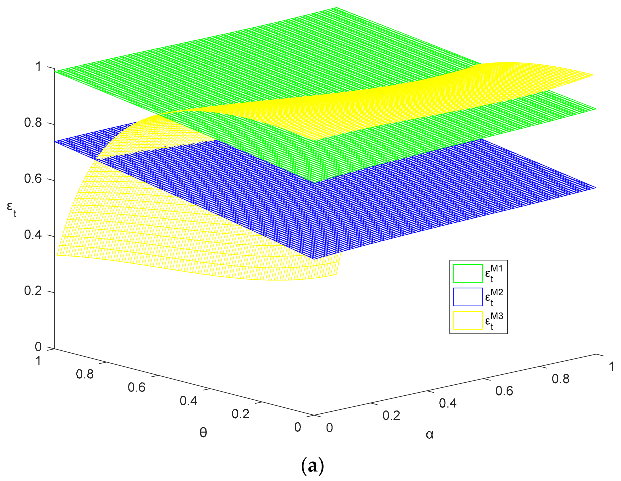
Figure 3a illustrates the impact of both
on OEM’s return rate. If dual competitions are not fierce,
is the largest. As
rise in value, OEM’s return rates are all decreasing. Meantime,
will first be exceeded by
, and then be lower than
. Hence, compared with centralized model in M1, with the increase of competition intensities, no matter who leads the reverse channel, he will reduce the return rate slowly so as to maintain his performance of reverse channel.
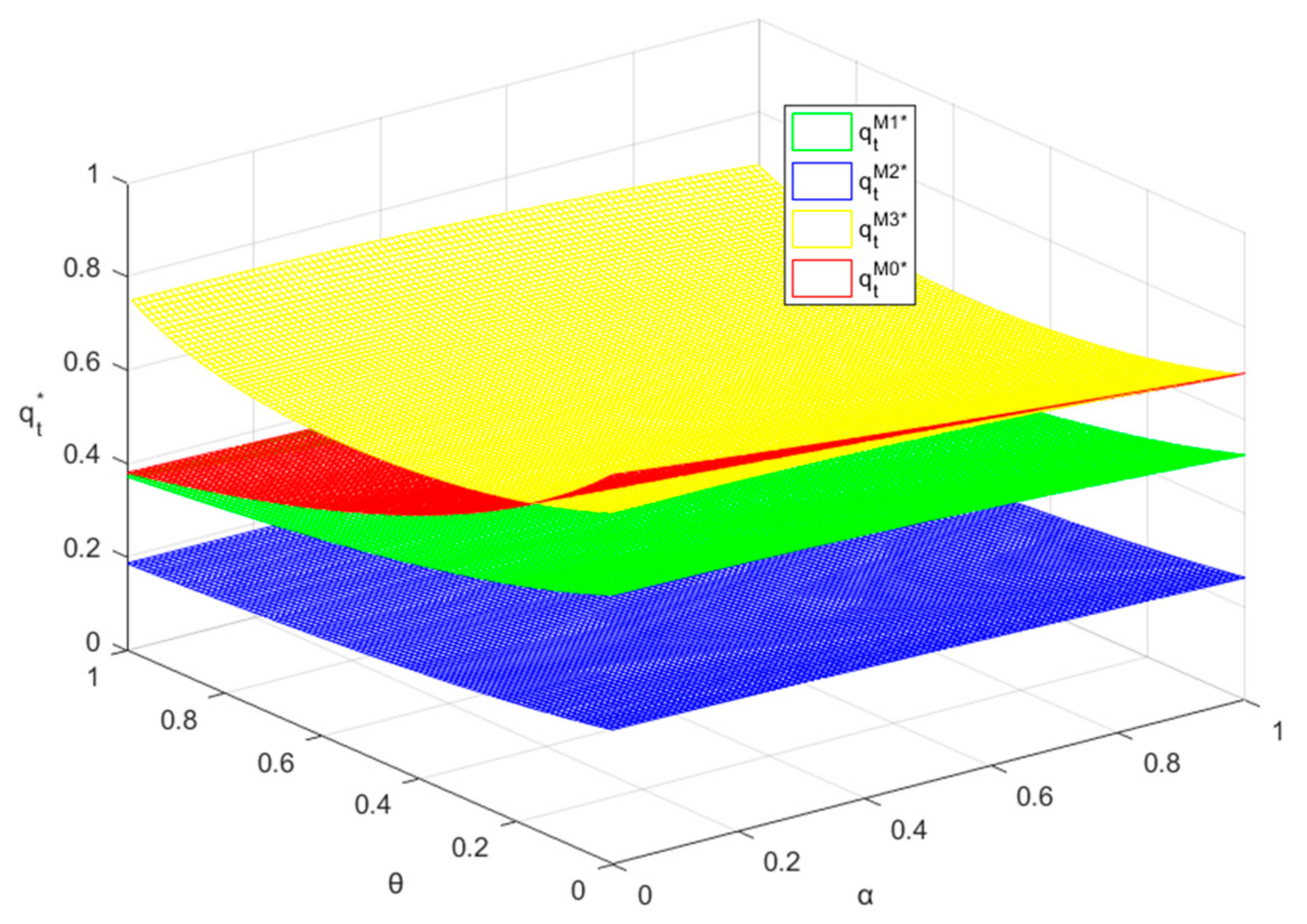
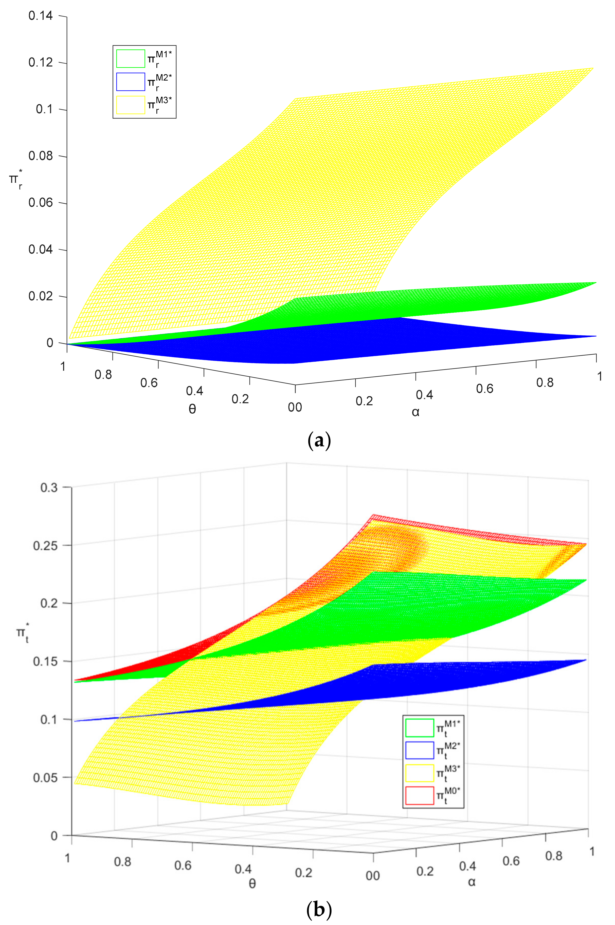
Proposition 3(iii) lists the comparison of total return rate between four models. The total return rate can be viewed as the performance of reverse channel. It is determined by OEM and the collector. By Proposition 3(iii), several interesting conclusions could be obtained. First,
is the largest, while
is the smallest. This implication is that the performance of reverse channel is affected by the forward power configuration. Since the collector is farther from the market, he has to tradeoff between higher transfer price and better total performance if he leads the reverse channel. If he leads the whole CLSC, he prefers higher transfer price. Otherwise, larger total return rate is better. Second, by
Figure 3, as
goes up, all the return rate decrease. Namely, the performance of reverse channel is worse off and even decreases to zero. In the worst case, reverse channel will be closed.
5.2. Forward Competition
Next, we give some comparative results between these models.
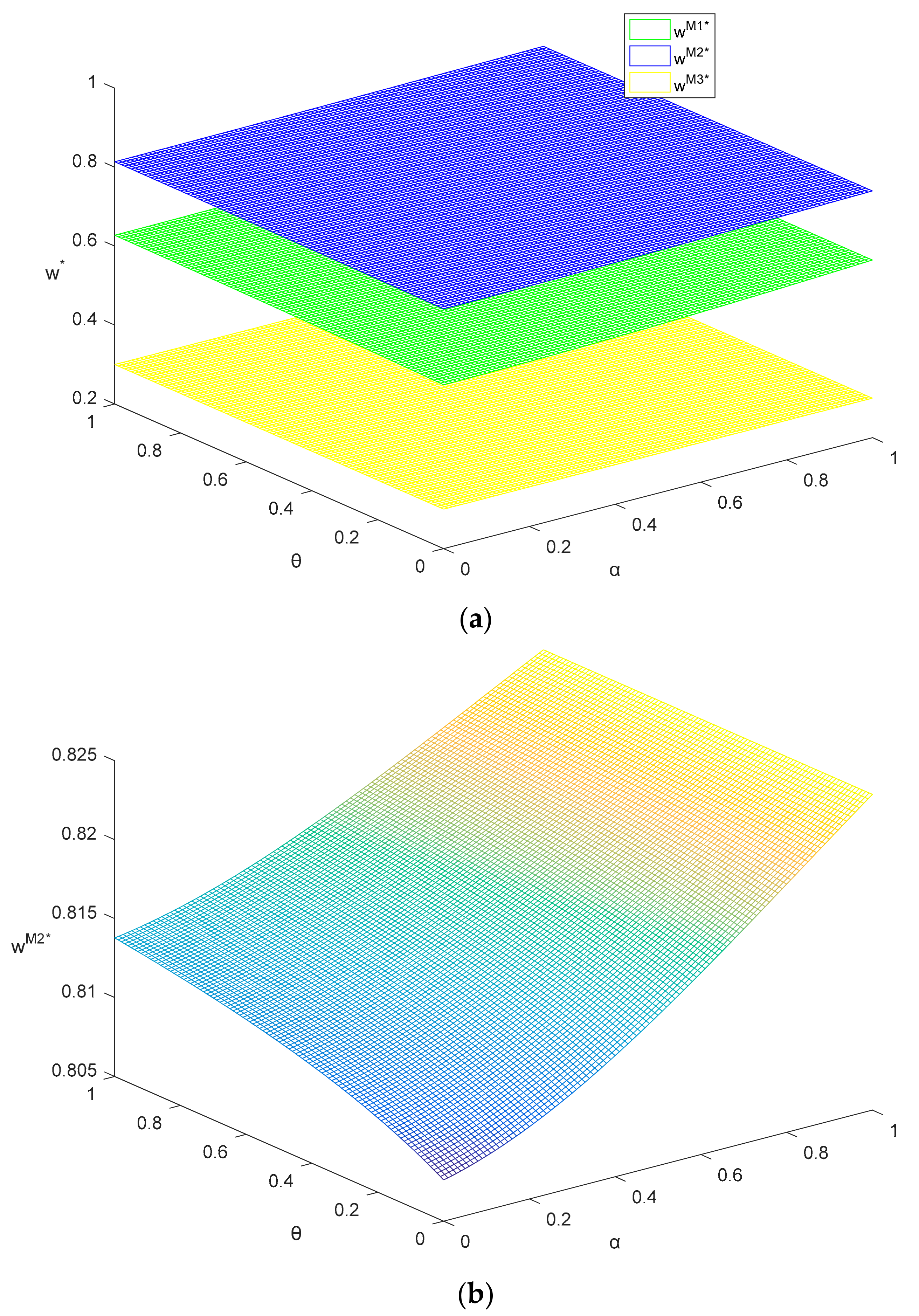
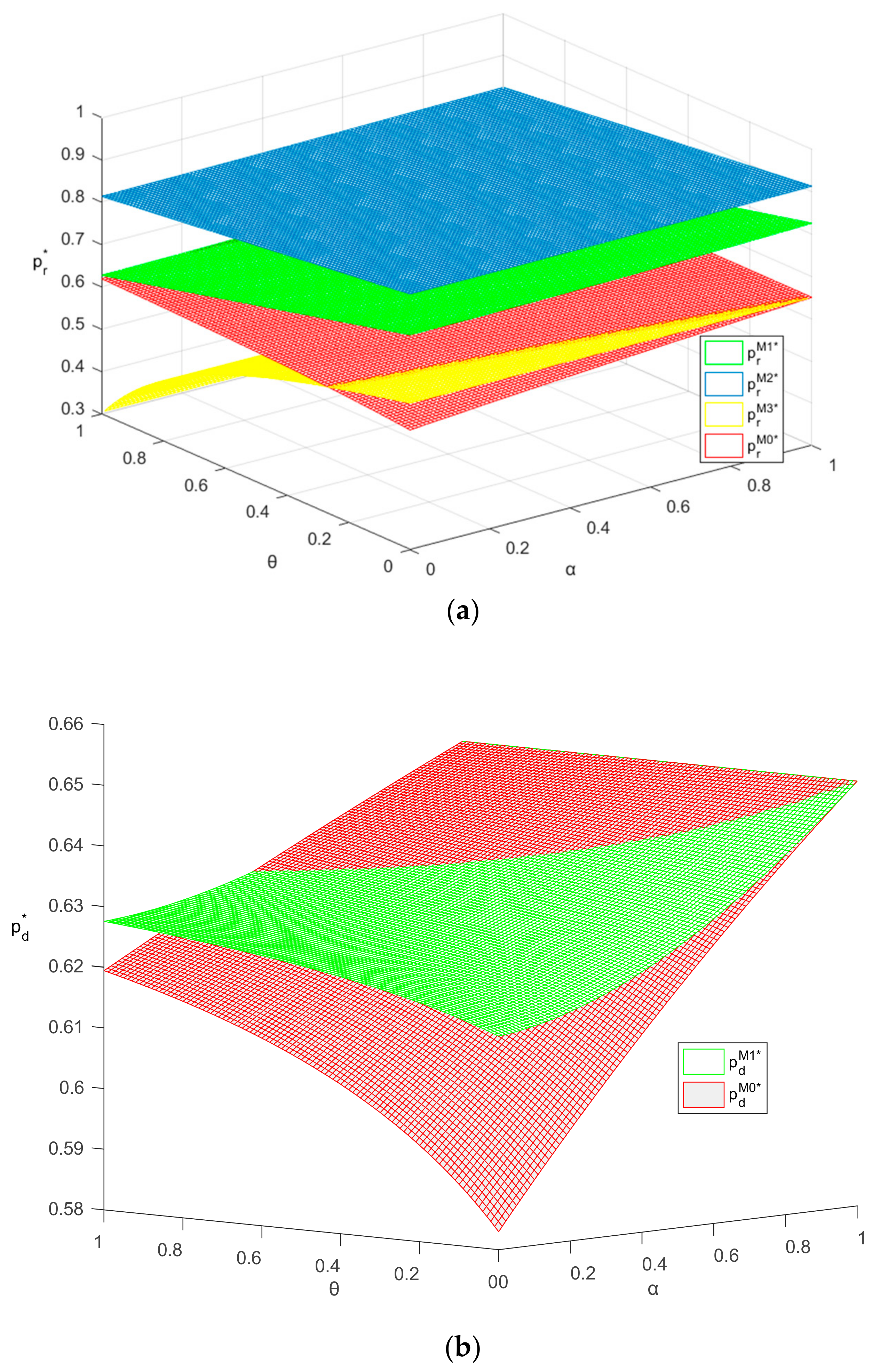
Proposition 4. The optimal wholesale prices satisfy .
It is intuitive that the wholesale price is smallest when the retailer leads the forward channel because he has strong incentive to cut the wholesale price. Furthermore, if OEM is incapable of selling the products directly, he might get nothing in the forward channel since the wholesale price offered by the retailer is even equal to OEM’s total cost. The wholesale price is highest in M2 since the forward channel in M2 is affected by reverse competition. Faced with highest transfer price, OEM has to raise the wholesale price. Compared with has been distorted further.
Figure 4 illustrates the wholesale price. By
Figure 4a, we can know the wholesale price lies on different levels when OEM holds different configurations. Namely, from the perspective of the retailer, his cost varies in different model. And the gap between different levels is so large that the ranking of the wholesale price is independent of competition intensities in both channels, even though every wholesale price is affected by both
. We take
for the example. First, the wholesale price is offered by OEM. As
goes up, he will raise the wholesale price in order to increase the retailer’s cost. Then his competitive advantage has been strengthened while the retailer’s has been weakened. It notes that as
goes up, the wholesale price is also increasing. Because the transfer price offered by OEM increases sharply with the increase of
, then OEM has to charge higher wholesale price from the retailer. Namely, the reverse competition affects the forward channel.
Proposition 5. (i) The optimal retail prices are ordered as follows: . If and only if and are smaller, . (ii) The optimal direct prices are ordered as follows: . If and only if and are larger, ;if and only if and are smaller, .
By Proposition 5(i), it is intuitive that the optimal retail price is lowest in Model M3 given his cost, i.e., the wholesale price is lowest. Besides, the wholesale price can be viewed as the cost of the retailer’s forward channel. Then the ranking of retail price between is consistent with that of wholesale price. Similar to Proposition 3, we find that retail price in M-(R-)led model outperforms (underperforms) that in the centralized model.
By
Figure 5a, if both competitions become fiercer, the retailer has a full control over the retail channel in Model M3 and he has a strong incentive to charge a lower retail price so as to increase the retail channel competitiveness. Under decentralized models, i.e., M1, M2, M3, retail price goes down as competition increases. However, the retail price in the centralized model increases with
. Because the integrated firm sets identical channel prices to maximize total quantities.
Proposition 5(ii) reveals the comparison of optimal direct prices. If OEM leads the forward channel, the wholesale price, offered by him, will be equal to the direct price. If unequal, the retailer will choose the lower one. Then OEM faces up with the tradeoff between lower direct price and higher wholesale price. By Proposition 5(ii), the direct price in Model M2 is higher than it in Model M1. If the forward channel is led by the retailer, OEM’s direct price will not be constrained by the wholesale price. The wholesale price offered by the retailer in M3 is so low that has the same ranking of direct price.
It is also interesting to observe that optimal direct price in M0 could be regarded as one boundary. Below the boundary, the retailer holds the first position; otherwise, OEM leads the forward channel. By
Figure 5b, if both competition intensities become increased, direct price grows. Faced up with the tradeoff between decreasing direct price and increasing the retailer’s cost, the latter impact dominates. However, if the retailer leads the channel, direct price in M3 goes down. OEM has strong incentive to charges a lower direct price so as to increase the direct channel competitiveness. Since the cost gap between two sellers is not that large in M3, the direct price drops sharply as the competition grows.
To sum up, when transfer price in M2 is adequately high, all the forward prices, including wholesale price, direct price, and retail price, are all highest. Second, as the competition grows, the retailer prefers to cut down the price, while OEM’s power configuration determines his behavior. If he holds the first position, he chooses to raise his price; otherwise, he has to cut his price. Besides, if OEM leads the forward channel, the cost gap between both forward members is so large that their competition is not in the same level. However, if the retailer takes control of wholesale price, his cost will be close to OEM’s. Then they will engage in a price battle. According to Proposition 4, we can get Corollary 2, which will further illustrate the final outcome of this price battle.
Corollary 2. (i) The optimal quantities of the direct channel satisfy . If and only if and are smaller, ; (ii) The optimal quantities of the retail channel satisfy ; (iii) The optimal total quantities satisfy . If and only if and are larger, ; if and only if and are smaller, . (iv) The optimal proportions of channel quantities satisfy , where , .
Corollary 2 discuss the comparisons of different kinds of optimal quantities. The results are consistent with the change of each prices. Sales quantities could be regarded as the performance of forward channel. Intuitively, the quantity is the lowest in M2 since the transfer price is such large that all the forward prices go up. The quantity is the largest in M3 if the retailer takes control of forward channel. If the competition is not that fierce, the quantities in M0 is largest. As the competition levels up, the quantities in M0 is decreasing and even exceeded by that in M1.
Figure 6c illustrate the impact of
and
on the total quantities. Generally speaking, as the competition goes up, no matter forward or reverse channel, sales quantities are decreasing in all the models but M3. This indicates competitions hurt the whole CLSC.
Figure 6 and
Figure 7 illustrates the impact of both competition intensities on the direct quantities and retail quantities. With the increase of forward competition, the forward power configuration plays the key role. To be more specific, the power of offering the wholesale price is the key factor. If OEM leads, he prefers to raise the wholesales to beat the retailer’s channel competitiveness. Meantime, the direct price also increases so that the direct quantities decrease in M1 and M2. Otherwise, as the forward follower, OEM will reduce his direct price to improve his own competitiveness. Then the direct quantity goes up in M3. OEM sells the products with low profits for big quantity. On the contrary, by Proposition 4, even though the retail price decrease in all the three decentralized models, all the retail quantities are not increasing but decreasing. Because the retail quantities depend on not only their retail price, but also OEM’s direct price. Surprisingly, the decreasing trend sustains no matter who leads the forward channel. If the retailer leads, the decrease of direct price is faster; if OEM is the leader, the decreasing of retail price is just a bit due to higher and higher wholesale price.
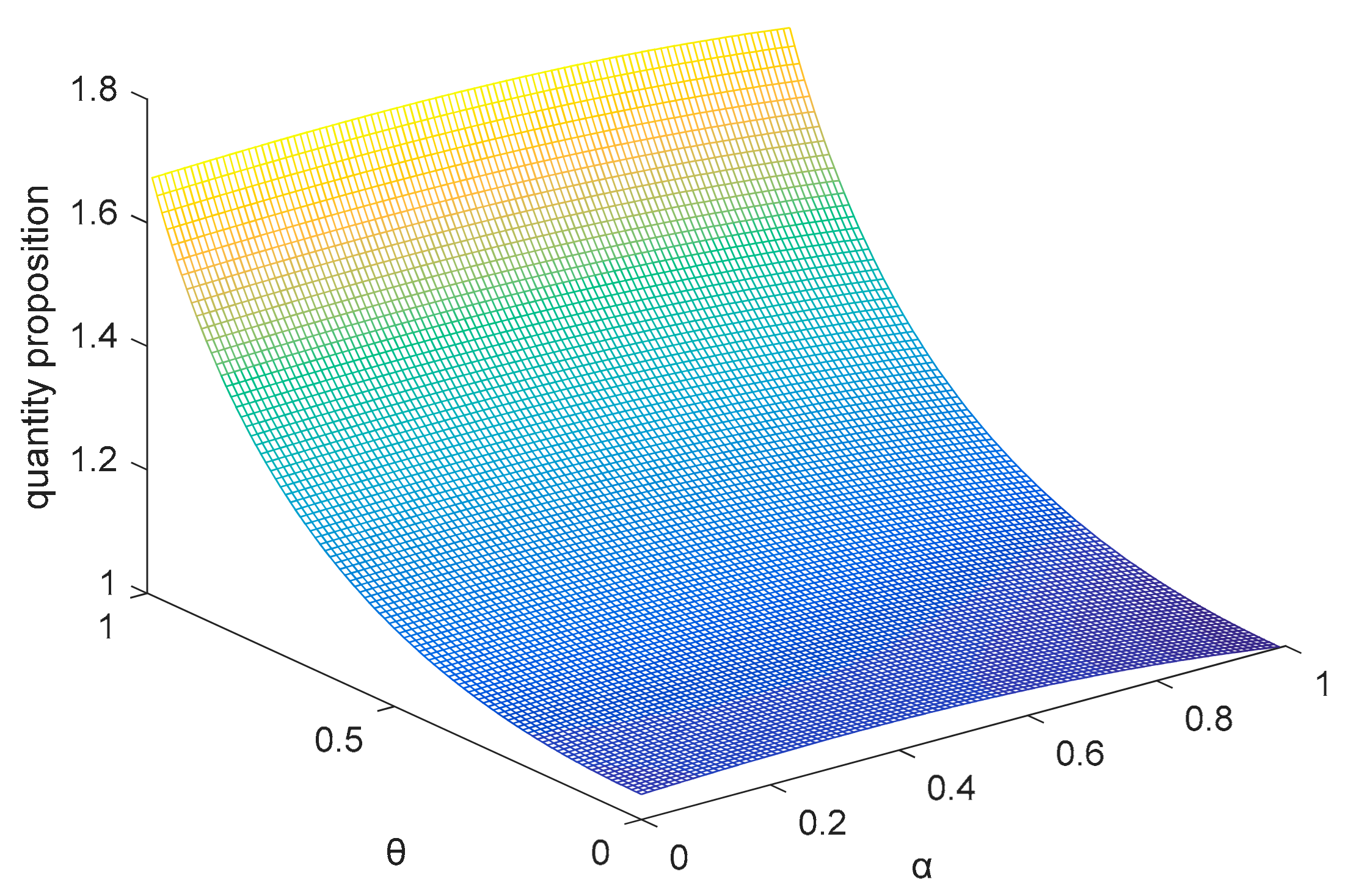
Corollary 2(iv) indicates the optimal proportions of channel quantities only depend on the forward power configuration in
Figure 8. The proportion can also be regarded as the channel share. Specifically, the proportion is
and only depend on the forward competition intensity if OEM leads the forward channel. However, if the retailer is the leader, the optimal proportion must be less than
and might arrive at 1 which is the optimal proportion in the centralized model. Unlike the proportion in the model led by OEM, it decreases in
while increases in
. Then OEM’s channel share becomes larger.
Now we discuss plausible reasons. If the forward channel led by the retailer, the price battle boosts the total quantities so that OEM’s return rate rises up and his cost reduces. OEM has more incentive to reduce the direct price. In contrast, the retailer’s cost is constant so that his retail price is higher. Then his channel share becomes smaller. If OEM leads the forward channel, faced up with more and more fierce competition, he takes the strategy of offering a higher wholesale price. Even though his direct price is also increasing while the retailer’s cost increases too. This results in the weaker channel competitiveness of the retailer. Then his channel share is also decreasing.
5.3. Dual Competitions
In this section, we first compare different equilibrium profits so that we can analyze CLSC efficiency. In addition, we investigate the extension of M3.
5.3.1. Comparison of Equilibrium Profits
Proposition 6. (i) OEM’s, retailer’s and collector’s optimal profits satisfy the following relationships: . If and only if and are larger, . (ii) ; ; (iii) Total channel profits are related as: . With the increase of and , first, , then, .
Intuitively, each channel member obtains the highest profits when they play the leader’s role, respectively. Moreover, from the perspective of CLSC, the profit in the centralized model is the highest. Because all decision variables are fully coordinated and there is no efficiency loss.
From OEM’s perspective, his profit is not the lowest when he holds both second positions in both channels. Even though he leads the forward channel in M2, losing the power of transfer price for him indicates that he might be at an inferior bargaining position to the collector. On the contrary, though his profit from reverse channel and retail channel are both zero, he can still benefit from his direct channel. As
goes up, his profit in M2 exceeds that in M3 due to price battle between him and the retailer. Result of battle is that both members’ profits are zero and total quantity attains maximum.
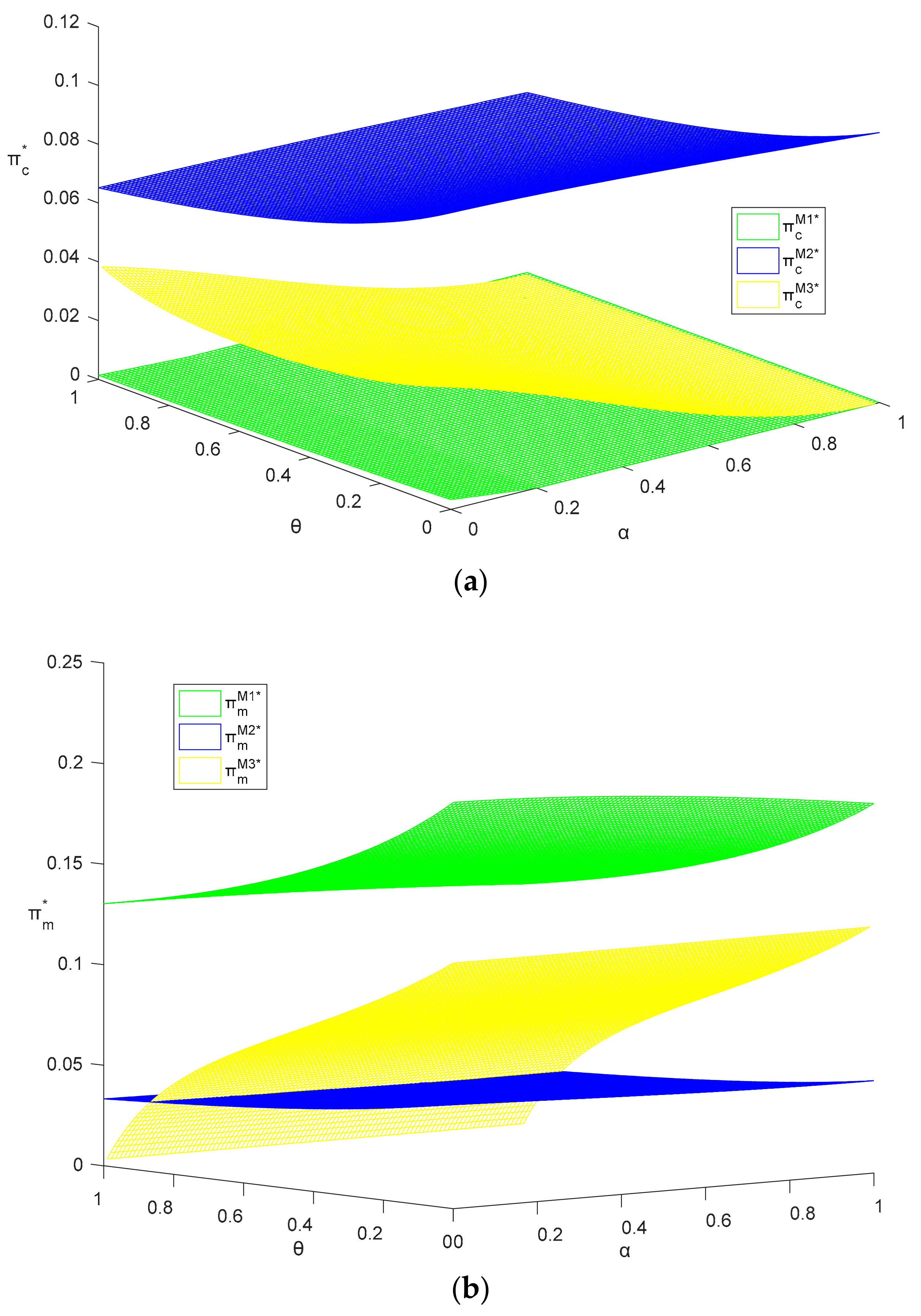
Figure 9b shows the impact of
and
on OEM’s profit. Intuitively, his profit will decrease in
, no matter the price war wages in the forward channel. If he leads the forward channel, his profit decreases owing to decreasing sales quantities. Otherwise, his decreasing profit implies that increasing direct quantities cannot offset the loss of decreasing unit profit margin. Moreover, his profit will also decrease in
, no matter who leads the reverse channel. Because decreasing reverse return rate results in increasing forward production cost. In summary, both competitions affect OEM’s profit, regardless of its power configuration.
From the retailer’s perspective, the ranking of his profit is aligned with that of his position.
Figure 10a shows that his profit declines in competition intensities and eventually tends zero. Likewise, from the collector’s perspective, similar conclusion could be drawn. Clearly, leading whole CLSC is different from leading single reverse channel. The collector has to share the first power with the retailer in M3 so that his profit depends on the negotiation with the retailer. We will discuss the question in next part.
Proposition 6(ii) shows that total profit is the highest in the centralized model owing to no efficiency loss. It is interesting to focus on the following two points. First, when and are smaller, total profit in M3 is so close to that in the centralized model. To optimize the performance of reverse channel, the collector will take the same perspective as does the whole CLSC and his return rate is equal to OEM’s. Meantime, in the forward channel, the retail price is nearly equivalent to the direct price so that the market size is shared equally. Therefore, both channel in M3 is consistent with that in M0. Second, when and are sufficiently high, total profit in M1 is rather close to that in M0. Specifically, if both competition is maximal, i.e., , , total profit in M1 is equal to that in M0. Namely, to hold both first power position for OEM can coordinate CLSC. The implication is that if competitions are fierce, to hold both first positions for OEM is preferred. Otherwise, both opponents will take actions simultaneously so as to maximize their own profits. Namely, from the perspective of CLSC, it is better to concentrate both powers to one OEM. Naturally, when competitions are smaller, it is optimal to hold both second position in both forward and reverse channels for OEM.
5.3.2. Analysis on CLSC Efficiency
Proposition 6(ii) sheds light on CLSC efficiency under dual competitions and power configuration. Then we can obtain Corollary 3.
Corollary 3. Supply chain efficiency is ordered as: . With the increase of and , first, , then, .
By Corollary 3, we can know the ranking of CLSC efficiency is consistent with that of total profit. It notes the worst CLSC efficiency comes in M2 due to “repeated double marginalization” [
7]. Classical double marginalization implies that the wholesale price which is higher than production costs leads to the efficiency loss. If the collector leads the reverse channel in M2, he offers so high transfer price that OEM has to raise the wholesale price. Therefore, “repeated double marginalization” includes two parts, i.e., between collector and OEM in the reverse channel, OEM and retailer in the forward channel.
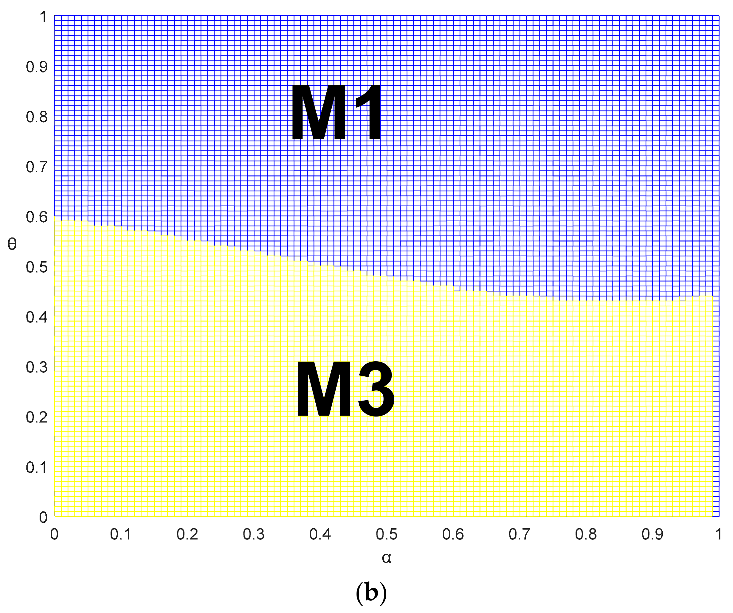
Besides, we analyze the relationship between M1 and M3. In M1, OEM leads both channel while he is follower in both channels in M3. From OEM’s perspective, M1 and M3 are just complementary. By
Figure 10b, we can obverse that the performances in both M1 and M3 are far higher than that in M2. Unlike M2, M1 and M3 get rid of “repeated double marginalization” since the condition of the latter is that there is a sequential game between wholesale price and transfer price. But there is either Nash game or no game in M1 and M3. Then M1 and M3 might just suffer from classical double marginalization problem. By
Figure 11a, if both competition is maximal,
. And if there are nearly no competitions,
is close to 1.
Figure 11b illustrates there exists a threshold line of
and
between M1 and M3. Above the threshold line, M1 is preferred; below the line, M3 outperforms. Besides, the observation is that
and
have the substitution effect since total profit in M0 decreases in both
and
. Then the threshold line indicates
decreases in
.
5.3.3. Extension of M3
Unlike OEM who controls both channels in M1, the collector and retailer in M3 lead the reverse and forward competition, respectively. In our analysis for M3, to ensure OEM’s participation, wholesale price is equal to production cost while the transfer price only depends on the reserve competition. Then the collector’s and retailer’s profit just come from single competition so that “repeated double marginalization” disappears. If OEM’s profit is always zero, we can explore the relationship between wholesale price and transfer price. For brevity, we just take unilateral competition into consideration, i.e., , and we can obtain the following theorem.
Theorem 5. If , , where.
By Theorem 5, we can know wholesale price increases in transfer price. Higher transfer price result in collector’s higher profit, and higher retailer’s profit comes from lower wholesale price. Intuitively, Theorem 5 indicates there is the inverse relationship between the collector’s profit and retailer’s profit. Likewise, Corollary 3 indicates the relationship between wholesale price and transfer price is also positive correlation so that there is “repeated double marginalization” in M2. Different from the case in M2 where the collector is the unique leader, the retailer in M3 also holds the first position. Then it is a key factor for comparison of the retailer’s and collector’s power. If collector has more power, M3 tends to be M2 and “repeated double marginalization” will be more serious so that M3 will be distorted from the full-coordinated channel in M0 more heavily.


