Article

Sky Luminance Measurements Using CCD Camera and Comparisons with Calculation Models for Predicting Indoor Illuminance

Department of Architecture, College of Engineering, Korea University, 145 Anam-Ro, Seongbuk-Gu, Seoul 02841, Korea
*
Author to whom correspondence should be addressed.
Sustainability 2018, 10(5), 1556; https://doi.org/10.3390/su10051556
Submission received: 4 April 2018 / Revised: 30 April 2018 / Accepted: 10 May 2018 / Published: 14 May 2018

Abstract

:
In this study, we address the algorithm of the calculation formula from sky luminance distribution to vertical illuminance and indoor illuminance. To predict daylight, studies about sky luminance distributions and the DeLight daylight model were investigated. This paper compared three well-known sky distribution models (Perez model, Igawa model, and CIE standard sky model) with measured data. The charge coupled device (CCD) camera was used as a measurement method for sky luminance distribution. Indoor illuminance values calculated with those well-known sky distribution models are compared with measured indoor illuminance data. The following conclusions were obtained: (1) In the results of R2, mean bias error (MBE), and Cv(RMSE) analysis, the CIE standard sky model showed the lowest error rate with measured data. Between the Perez model and Igawa model, the Igawa model showed a lower error rate; (2) When we compared the sky classification of the Perez model and the Igawa model, both models classified the sky similarly to the CIE standard sky model in March. However, the classification of the sky in the CIE standard sky model, the Perez model, and the Igawa model differed in some of the July data because of high solar elevation; (3) The illuminance of the center point of the room was calculated using the well-known sky luminance distribution model, the Igawa model has a lower error rate than the Perez model in Korea.

1. Introduction

Buildings account for approximately 40% of the world’s annual energy consumption, while lighting the interior environment contributes the largest portion to building energy consumption [1]. To reduce lighting energy consumption, it is important to forecast the indoor illuminance at the early design stage. If you are predicting indoor illuminance in the initial design stage, you can place light-based eco-friendly systems, such as a photosensor, to calculate energy savings accordingly [2]. When installing artificial lighting, it can be installed considering the indoor light environment so that efficient lighting design becomes possible [3,4,5]. Important input data for predicting the indoor illuminance are the distributions of the sky luminance. Many studies have been carried out to develop models for categorizing and calculating sky luminance distribution, including the Perez model by Perez et al. [6], the International Commission on Illumination (CIE) standard general sky model by Kittler [7], and the all sky model by Igawa [8].
Many researchers have evaluated a number of sky luminance distribution models [9,10,11,12,13]. Torres et al. [14] studied the daylight conditions in Pamplona. They used two-year data of luminance distribution for selecting the sky type, and found that the most frequent sky type in Pamplona is CIE standard clear sky, polluted atmosphere. Ferraro et al. [15,16] analyzed the sky conditions in Italy, France, and Japan using a sky scanner and compared the results with those obtained with the CIE standard general sky, Perez model, and Igawa model. The CIE standard general sky model showed more similar results with the measured values than the Perez model and the Igawa model. Chauvin, et al. [17] studied the prediction of various sky conditions using a sky imager, having an economical and time-saving advantage over using a sky scanner. After comparing images of various sky conditions of a representative clear sky, they investigated a way to classify sky conditions by detecting the cloud region. When compared with the algorithm based on Perez’s All-weather model, a 15% error reduction in the entire sky and a 20% error reduction in the solar orbit were observed. The vertical illuminance value is important for indoor illuminance prediction, and the sky distribution model is the important factor for the vertical illuminance value. Li et al. [18,19] verified the formula for predicting each vertical surface illuminance with sky luminance data, and studied a graphical method for calculating the internal illuminance for the CIE standard clear sky using daylight counting.
In this study, the process of applying the well-known sky model to vertical surface and indoor illuminance prediction formulae are analyzed and compared with the actual measurement data. The diffuse component is considered the greatest potential source of error in the calculation of illuminance [14]. The diffuse component is mainly influenced by sky luminance distribution seen in the field of view of the window. We focused on the diffuse component to analyze error in illuminance prediction. Sky luminance distribution is influenced by weather and climate as well as luminance distribution changes during the day with solar position [20]. Clouds and turbidity also play key roles in regulating the level of solar irradiance [21,22]. Therefore, how to calculate diffuse components known to depend on sky luminance distribution may vary from region to region. In order to reduce error in calculating the diffuse component, it is necessary to measure sky luminance distribution everywhere in a comparatively easy way and apply the appropriate algorithm to each region. In this study, we analyzed the sky luminance distribution of Korea as a measurement area and presented a relatively simple method for measuring sky luminance distribution. In addition, we analyzed the error rate from sky luminance distribution to indoor illuminance prediction step by step.
The purpose of this study was to present a process to find a sky luminance distribution model appropriate for each region. The sky luminance distribution model selected by the method presented in this study was used to calculate vertical illuminance and indoor illuminance. The validity of the calculation process of the indoor illuminance using sky luminance distribution was verified by comparing measured vertical illuminance and indoor illuminance to calculated values. In this study, luminance measurements in Seoul, Korea, are used.
For forecasting indoor illuminance, this study included the following processes (Figure 1).
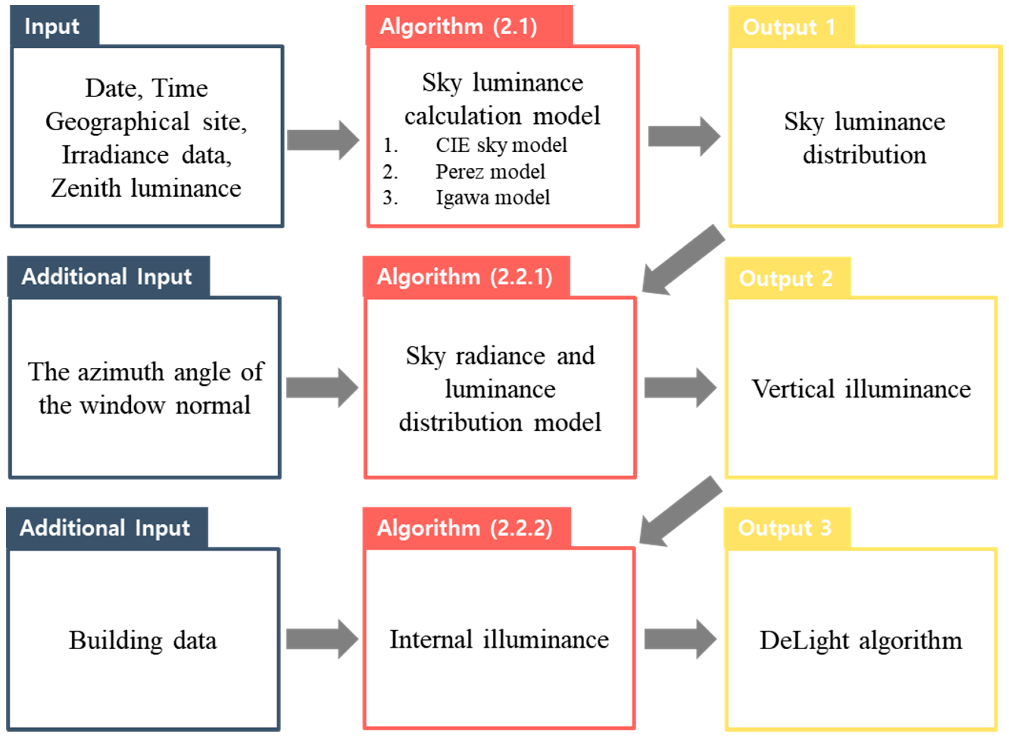
  • Use date, time geographical site, irradiance data and zenith luminance to calculate luminance distribution of the sky. The CIE standard sky model, Perez model, and Igawa model were used for this calculation. Calculated luminance distributions were compared with luminance distribution measured with high dynamic range images (HDRI) to evaluate the accuracy of the sky distribution model.
  • Calculate vertical illuminance of window surface by adding orientation of the window to luminance of each part of the sky calculated from the sky distribution model and compare it with the measured value.
  • Calculate indoor illuminance by adding space data to vertical illuminance calculated in step 2. The calculated indoor illuminance was then verified against measured values

2. Theory

2.1. Sky Luminance Calculation Models

Well-known models for the calculation of sky luminance distributions are the Perez model, Igawa model, and CIE standard sky model. The following formula for defining the relative luminance distribution was proposed by Kittler et al. [23]. The standard formula defining the ratio of relative sky luminance to zenith luminance for any standard sky can be considered by combining a gradation function and indicatrix function, as follows:
Lγα/Lz = [f(χ)φ(Zi)]/[f(Zs)φ(0°)]
where
  • Lγα is the luminance of the sky patch [cd/m2],
  • Lz is the luminance of zenith [cd/m2].
A sky patch is a single piece of a divided hemisphere. For calculating Lγα, the relative indicatrix function f and the relative gradation function φ are needed in Equation (1). The relative indicatrix function f gives the relation of the relative luminance of a sky patch to its angular distance from the sun. The luminance gradation function, φ gives the relation of the luminance of a sky patch to its zenith angle [24]. φ and f are defined in Equations (2) and (3):
f(χ)/f(Zs) = [1 + c{exp(dχ) − exp(dπ/2)} + e(cos2χ)]/[1 + c{exp(dZs) − exp(dπ/2)} + e(cos2Zs)],
φ(Zi)/φ(0°) = {1 + a exp(b/cosZi)}/{1 + a × exp(b)},
where
  • Zi is the zenith altitude angle of the sky patch [radians],
  • Zs is the solar zenith angle [radians],
  • a, b, c, d, and e are the coefficients applied differently for every calculation model,
  • χ is an angular distance between the sky patch and the sun.
χ can be calculated as follows:
χ = arccos(cosZs × cosZi + sinZs × sinZi × cos|αi − αs|)
where
  • αi is the azimuth angle of the sky element [radians],
  • αs is the solar azimuth angle [radians].
For the measurement and calculation of the sky luminance distribution, the hemispherical sky was divided into 145 patches according to the CIE Guide [20].

2.1.1. CIE Standard General Sky Model

Kittler et al. [7] classified all sky conditions into 15 categories, and Darula and Kittler [25] proposed this calculation model. Subsequently, CIE recommended this model as the CIE standard general sky [20]. The International Organization for Standardization (ISO) accepted 15 international types of standard sky [26]. Each sky patch luminance value can be calculated using six kinds of indicatrix functions and six kinds of gradation functions, as in Equations (2) and (3), respectively. The combinations of the function types form the fifteen sky luminance distributions. The coefficients a–e used in the CIE standard sky models can be selected according to the sky condition [20].
However, CIE does not give clear criteria for each of the 15 types of sky independent of the luminance measurements [27]. The value of the ratio of the zenith luminance to the horizontal diffuse illuminance, Lz/EdH, is one of the proposed criteria of the choice of CIE sky types [25]. This criterion has been studied and showed validity only when the solar altitude is lower than 30 degrees [15]. If the solar altitude is higher than 30 degrees, it is difficult to select one category because there is an intersection in the graph. Our measurement was made at a latitude of 37.58° N and a longitude of 127.03° E. At this location, solar altitude angle is the highest on June 21, with a value of 75.8 degrees. Therefore, it can be said that the above method is not suitable for the criteria. Another way is to compare the indicatrix and gradation functions; however, this method is more difficult to apply than the previous method, and is not useful when the sun altitude is above 45 degrees [13].
We chose a method firstly proposed by Tregenza [24]. That method has no application limits, and needs knowledge of the measured luminances. This method compares the measured values with the 15 types of CIE standard sky, respectively, and then selects the sky with the minimum RMSE value [12,15,28]. In this paper, the CIE sky model was not used for the analysis of indoor illuminance. The CIE standard sky model requires more input values than the Perez model or the Igawa model because it can be evaluated by comparing luminance values of the whole sky distribution, which is a relatively inefficient calculation. Therefore, this model is not suitable for this study which evaluates a simple indoor lighting calculation formula. However, the CIE standard sky model in this paper can serve as a criterion for defining the state of HDRI by selecting sky state and comparing the whole luminance.

2.1.2. Perez Model

Perez et al. [6] proposed a sky distribution model that can be subdivided into 8 categories using the sky clearness index, ε. This value is defined as
ε = {(GdH+ GND)/GdH + 1.041 Zs3}/(1 + 1.041 Zs3)
where GdH is the horizontal diffuse irradiance [W/m2] and GND is the normal incident direct irradiance [W/m2]. The criteria for the eight categories classified by the sky clearness index ε: category 1 (1 < ε ≤ 1.065), category 2 (1.065 < ε ≤ 1.230), category 3 (1.230 < ε ≤ 0.500), category 4 (1.500 < ε ≤ 1.950), category 5 (1.950 < ε ≤ 2.800), category 6 (2.800 < ε ≤ 4.500), category 7 (4.500 < ε ≤ 6.200), category 8 (6.200 < ε).
Because the Perez model is defined by horizontal diffuse irradiance and direct normal irradiance, skies can be divided more specifically than with CIE standard general sky.
The Perez model uses the same equations as Equations (1)–(3), although the calculation methods of coefficients a–e differ to those with the CIE standard general skies. Coefficients a–e for the Perez model are calculated by the following equation:
x = x1 + x2Zs+ ∆[x3 + x4Zs]
This equation can be used for all coefficients except c and d of category 1. The equations of coefficients c and d for the first category are defined as
c = exp[{∆ (c1 + c2Zs)}c3] − c4
d = −exp[∆(d1 + d2Zs)] + d3+∆d4
where x1 to x4 are the coefficients proposed by Perez, and ∆ is the sky brightness.
Δ   =   m   ×   G dH / E es 0
where m is the optical air mass [29], and E es 0 is the normal incident extraterrestrial irradiance [W/m2].

2.1.3. Igawa Model

The sky radiance and luminance distribution model was proposed by Igawa et al. [8] for all sky conditions from clear sky to overcast sky. For this model, a method is proposed that categorizes sky conditions according to a sky index. The sky index (Si) value can be calculated from both the clear sky index, Kc, and the cloudless index, Cle. The clear sky index is defined based on the global irradiance. The cloudless index is defined based on the global irradiance and the diffuse irradiance. The sky index is defined as
Si = Kc + Cle0.5
Kc and Cle are calculated as follows:
Kc = GgH/Seeg
Cle= (1 − Ce)/(1 − Ces)
In the function of Kc, the values of the horizontal global irradiance [W/m2], GgH, and the standard global irradiance [W/m2], Seeg, are needed. The values of Seeg can be calculated using the following formula:
Seeg = 0.84 × (Eeo/m) × exp(−0.0675∙m)
In Equation (13), the extraterrestrial direct normal irradiance and m is the relative optical air mass [29]. Although the extraterrestrial direct normal irradiance, Eeo shows an error of ± 3% over time, in this paper we applied a constant value of 1367 W/m2 [8]. The sky conditions are classified into five categories: (1) clear sky conditions, (1.7 ≤ Si); (2) near clear sky conditions (1.5 ≤ Si < 1.7); (3) intermediate sky conditions (0.6 ≤ Si < 1.5); (4) near overcast sky conditions (0.3 ≤ Si < 0.6); and (5) overcast sky conditions (Si < 0.3).
In the function of Cle, the values of the cloud ratio, Ce, and the standard cloud ratio, Ces, are given by
Ce = GdH/GgH
Ces = 0.01299 + 0.07698∙m − 0.003857∙m2 + 0.0001054∙m3 − 0.000001031∙m4
For sky distribution, the Igawa model uses the same formulas as Equations (1)–(3). Unlike the CIE standard general skies model, the Igawa model uses calculation functions of coefficients a–e, similar to the Perez model. Each coefficient in the Igawa model is calculated using a single formula, regardless of the sky category. Therefore, the Igawa model can represent a continuous sky state. This is the big difference with Perez model. Coefficients a–e for the Igawa model can be calculated using the following equations:
a = 4.5/[1 + 0.15∙× exp(3.4∙Si)] − 1.04
b = (−1)/[1 + 0.17 × exp(1.3∙Si)] − 0.05
c = 1.77∙(1.22∙Si)3.56 × exp(0.2∙Si)(2.1 − Si)0.8
d = (−3.05)/[1+10.6∙× exp(−3.4∙Si)]
e = 0.48/[1+245∙× exp(−4.13∙Si)]
The criteria of the three sky distribution models and characteristics of the a–e constant that determines the sky distribution are summarized in Table 1.

2.2. Vertical and Interior Illuminance Prediction Algorithm

2.2.1. Sky Radiance Luminance Distribution Models for Vertical Illuminance

Since sunlight enters a room through windows, the prediction of the luminance or illuminance on the window can be considered as a preliminary step for predicting the indoor illuminance. In the DeLight algorithm [30], which predicts the indoor illuminance at a specific measurement point, the indoor illuminance is predicted by using the vertical luminance at the window as input. Therefore, the prediction of the vertical surface luminance is an important factor in predicting indoor daylight illuminance.
In this study, sky radiance and luminance distribution models were used to predict vertical surface illuminance using the calculated sky luminance values of 145 sky patches. Using an appropriate correlation of the diffuse and direct luminous efficacy, irradiance data can be converted to illuminance data [31]. Since the diffuse component of daylight is mainly influenced by sky luminance distribution, there is a limit to the conversion using efficiency. A suitable alternative to calculate the diffuse illuminance in the vertical surface is to integrate the portion showing sky luminance distribution [18]. The global illuminance on a vertical surface [lx], EgV can be evaluated as the sum of the direct illuminance on a vertical surface [lx], EDV, and the diffuse illuminance on a vertical surface [lx], EdV, and the ground reflected illuminance on a vertical surface [lx], Erg:
EgV = EDV + EdV + Erg.
Among the three elements of the global illuminance on a vertical surface, the diffuse illuminance on a vertical surface, EdV, can be calculated using the luminance value of each part of the sky patch calculated by each sky luminance distribution algorithm. The equation is as follows [19]:
E dV = i = 1 145 L γ α   cos 2 γ i   cos ( α i α n ) i δ γ δ α   ( 0 γ i π / 2 , π / 2 α i α n π / 2 ,   otherwise = 0 )
where
  • Lγα is the sky luminance of a sky patch [cd/m2],
  • γi is the altitude angle of a sky element [radians],
  • αi is the azimuth angle of a sky element [radians],
  • αn is the azimuth angle of a window normal [radians].
The direct illuminance on a vertical surface was calculated using the following equation [32,33]:
EDV = EDN cos γs cos|αs − αn|
EDN = 133800[1 + 0.033 cos(360J/365)] exp (−av m)|
where
  • EDN is the direct normal illuminance,
  • J is the Julian date, the value of which is from 1 to 365,
  • γs is the solar altitude angle [radians],
  • av, the mean extinction coefficient [34].
In the above equation, the mean extinction coefficient, av, is 0.32 for clear sky [30] and 0.8 for intermediate sky [32], whereas an overcast sky is not applicable since there is no direct element. The Perez model and the Igawa model, used in the calculation of the global illuminance on a vertical surface, each have three or more sky categories. Therefore, in the Perez model, categories 7 and 8 are classified as clear sky, and categories 3 to 6 are classified as intermediate sky. In the Igawa model, the clear sky and near clear sky were classified as clear sky, and the mean extinction coefficient, av was applied.
The ground reflected illuminance on a vertical surface is calculated using the following equation [35]:
Erg = Egρg/2
Eg = EdH + EDN sin γs, when cos γs cos (αn − αs) > 0
= EdH, otherwise
where Eg is the ground illuminance, ρg is ground reflectance, and EdH is the diffuse illuminance on a horizontal surface. ρg is 0.2, which is a general value. EdH can be calculated using the luminance value of each part of the sky patch calculated by each sky luminance distribution algorithm. The equation is as follows [19]:
E dH   =   i = 1 145 L γ α   sin γ i   cos γ i   δ γ   δ α

2.2.2. Algorithm of DeLight

In this study, DeLight of Vartiainen [30], one of the daylight prediction algorithms of Energy plus [36], was selected as an algorithm to predict the interior illuminance using the analyzed sky luminance distribution model. There are a number of algorithms that can calculate illuminance/luminance in indoor/outdoor spaces. The most representative ones are the ray tracing method and the radiosity method. These two methods are often used in 3D simulation tools because of their complexity of the calculation process. A relatively simple method is to calculate daylight rate which is the indoor illuminance ratio to outside global horizontal illuminance in the overcast sky. However, this method is only for overcast sky. Depending on weather conditions, it is difficult to know the illuminance value of the specific point in the room. The DeLight algorithm has a relatively simple computation process. Also, it has been suggested that the prediction accuracy is verified because it is selected as one of the algorithms of the EnergyPlus program. In the Vartiainen’s DeLight algorithm, the horizontal illuminance of the daylight entering a room can be calculated as the sum of the interior horizontal direct illuminance, the interior horizontal diffuse illuminance, and the interior horizontal reflected illuminance. The formula is as follows:
Ei = EDi + Edi + Eri
where
  • Ei is the horizontal illuminance of the daylight entering a room [lx],
  • EDi is the interior horizontal direct illuminance [lx],
  • Edi is the interior horizontal diffuse illuminance [lx],
  • Eri is the interior horizontal reflected illuminance [lx].
This formula can only be applied to vertical windows.
When direct sunlight affects the measurement point, the interior horizontal direct illuminance can be calculated as follows:
EDi = τw1) EDN𝑠𝑖𝑛 𝛾𝑠
where
  • τwi) is the light transmittance of the window with the angle of incidence γi [%].
  • θi is the light transmittance of the window with the angle of incidence [37].
The interior horizontal diffuse illuminance at the measurement point, Edi, can be calculated as follows:
E di = 0 w w 0 h w τ w L v zydxdy ( x 2 + y 2 + z 2 ) 2 = τ w L v 2 ( tan 1 w w z z h w 2 + z 2 tan 1 w w h w 2 + z 2 )
where
  • Lv is the luminance of the radiating surface [cd/m2],
  • x is the horizontal distance of the surface element from the left edge of the window [m],
  • y is the vertical distance of the surface element from the lower edge of the window [m],
  • z is the perpendicular distance of point P from the window [m],
  • r is the distance between point P and the surface element [m],
  • ww is the width of the window [m],
  • hw is the height of the window [m],
Lv is calculated by dividing the global illuminance on a vertical surface by π. The room geometry for calculating interior horizontal diffuse illuminance is depicted in Figure 2.

3. Methodology and Measurement

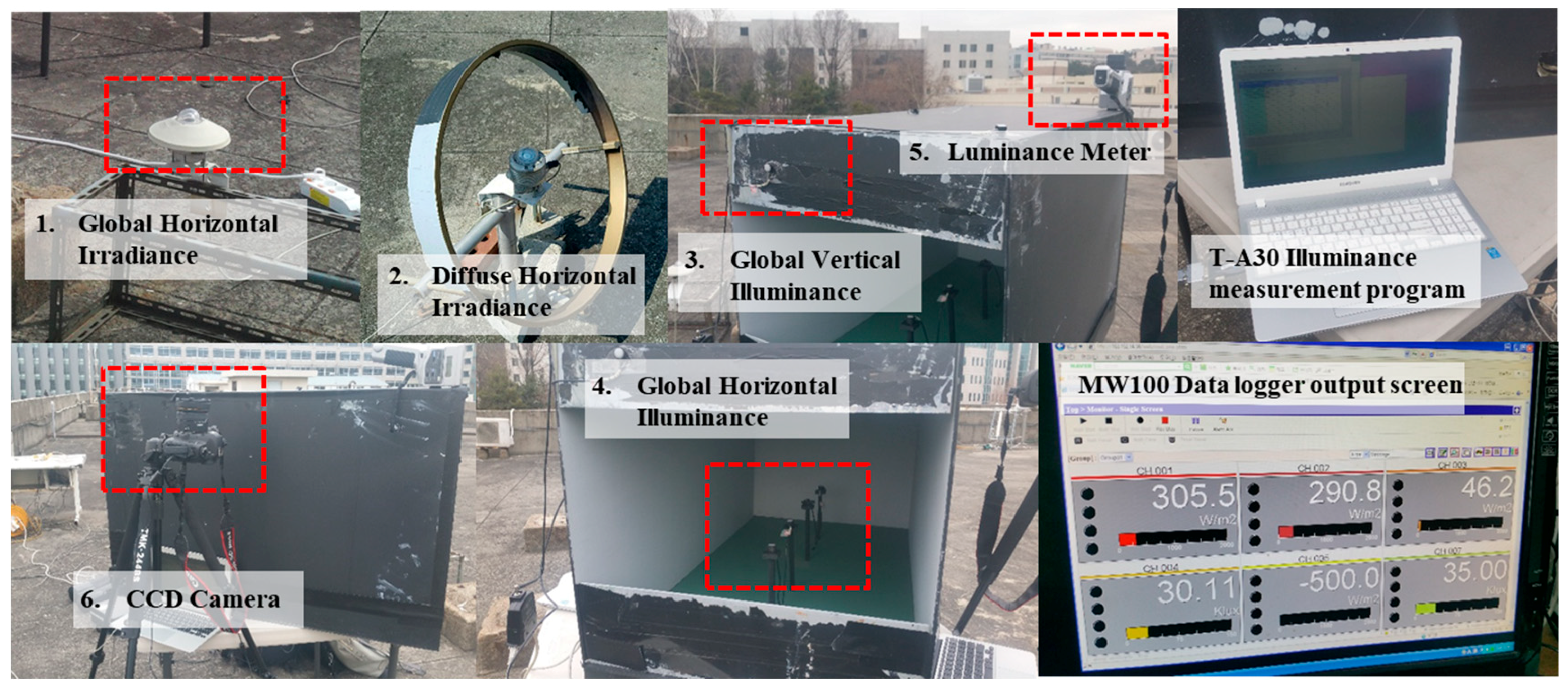
3.1. Measurement Method

To verify the measured indoor illuminance through comparison with the calculated values, sky luminance distributions need to be measured and analyzed. Various illuminance and irradiance values are needed. The measurement quantities for this study are listed in Table 2.
The global horizontal irradiance and the diffuse irradiance are measured at 1 s intervals for input data of the calculation models. Two irradiance sensors are installed in the rooftop of the College of Engineering building of the Korea University (Latitude: 37.58° N, Longitude: 127.03° E). These irradiance sensors are connected to the lab computer and data logger (MW 100). The data logger converts the measured value from sensors into an electrical signal and outputs it to the CF memory card in the data logger. Illuminance sensors are placed on the vertical surface, the horizontal surface, and the center point of the work surface height (0.8 m) of the measurement model. The illuminance sensors were calibrated to allow all sensors to measure the same value. The spot luminance meter used a calibrated standard value in Minolta. The global horizontal irradiance and the diffuse irradiance were measured using a pyranometer with shadow band. Correction to the shadow band is essential when making measurements using a pyranometer with a shadow band. In this paper, we corrected the shadow band using the method of Muneer and Zhang [38].
Device pictures used for measurement are shown in Figure 3.
The size and reflectance values of the room used in the measurement are shown in Table 3.
The scale of measurement model for interior illuminance is 1:5. This scale model has been set with reference to a common small office form in Korea. The center of the space is important because it can represent the entire interior illuminance [39]. Therefore, we selected and analyzed indoor illuminance for the center of the space as a representative illuminance. A charge coupled device (CCD) camera was used to capture the sky image and a spot luminance meter was used to measure the zenith luminance value shoot at 10 min intervals. The CCD camera is capable of a partial analysis of a limited area, rather than only the entire sky, and it can obtain digital images. The CCD camera has advantages over a sky scanner in response speed and price [40]. The CCD camera consists of a fisheye lens and a digital single lens reflex (DSLR) camera [41].

3.2. Description of the Methodology

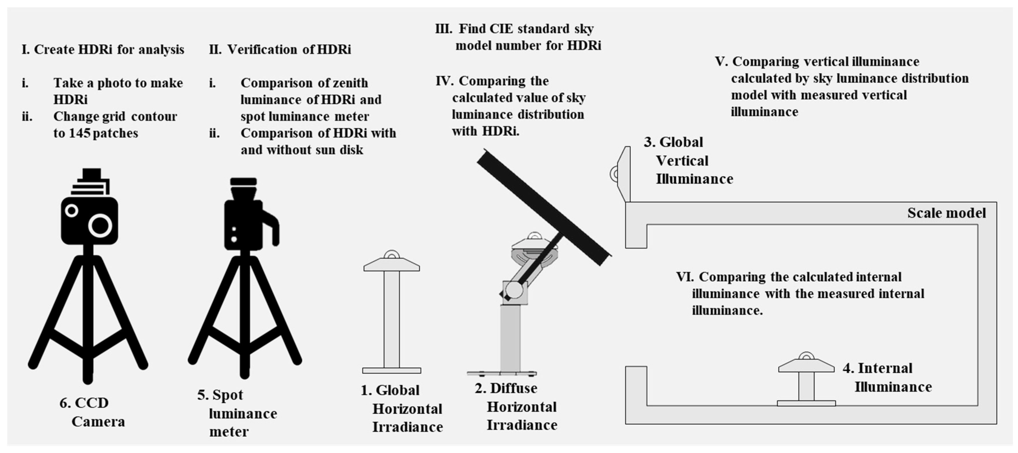
3.2.1. The Process of Analyzing Measurements

A description of the experimental procedure and the methodology of the study using experimental data are shown in Figure 4.
First, three pictures were taken to create an HDRI using a CCD camera. Photographed images were combined in the form of HDRI and verified by comparison with zenith luminance measured with a spot luminance meter. Sky grid shape luminance contour analyzed by HDRI has been changed to 145 patch luminance contour through the conversion process (Section 3.2.2). We calculated sky luminance distributions of the Perez model and the Igawa model using the measured global horizontal irradiance and global diffuse irradiance. Sky luminance distributions of the calculated Perez model and Igawa model were compared with measured values of HDRI. CIE standard sky model selected through comparison with each luminance of 145 patches of HDRI was also compared and analyzed. Vertical illuminance was calculated by integrating sky luminance distribution seen from the vertical plane. We compared calculated results with measured vertical illuminance to verify the effect of sky luminance distribution on vertical illuminance. Finally, we calculated indoor illuminance using vertical illuminance and compared the calculated indoor illuminance with the measured indoor illuminance. Since sky luminance distribution could affect the diffuse component, we further analyzed overcast sky known to be less influenced by direct component.

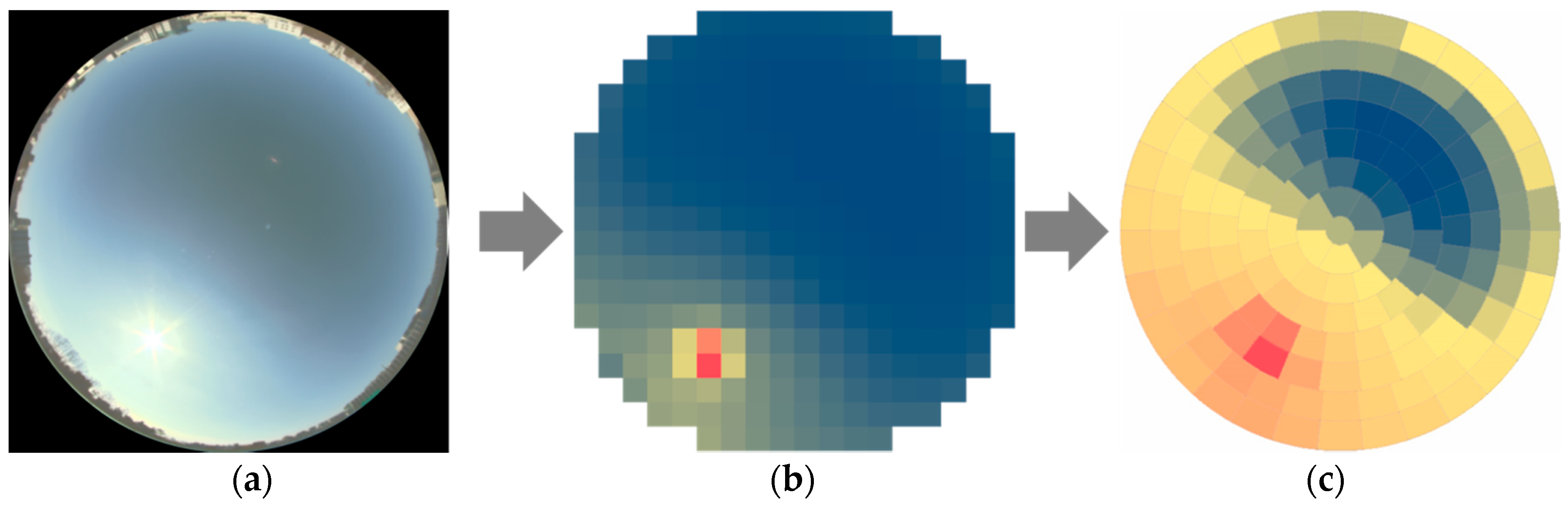
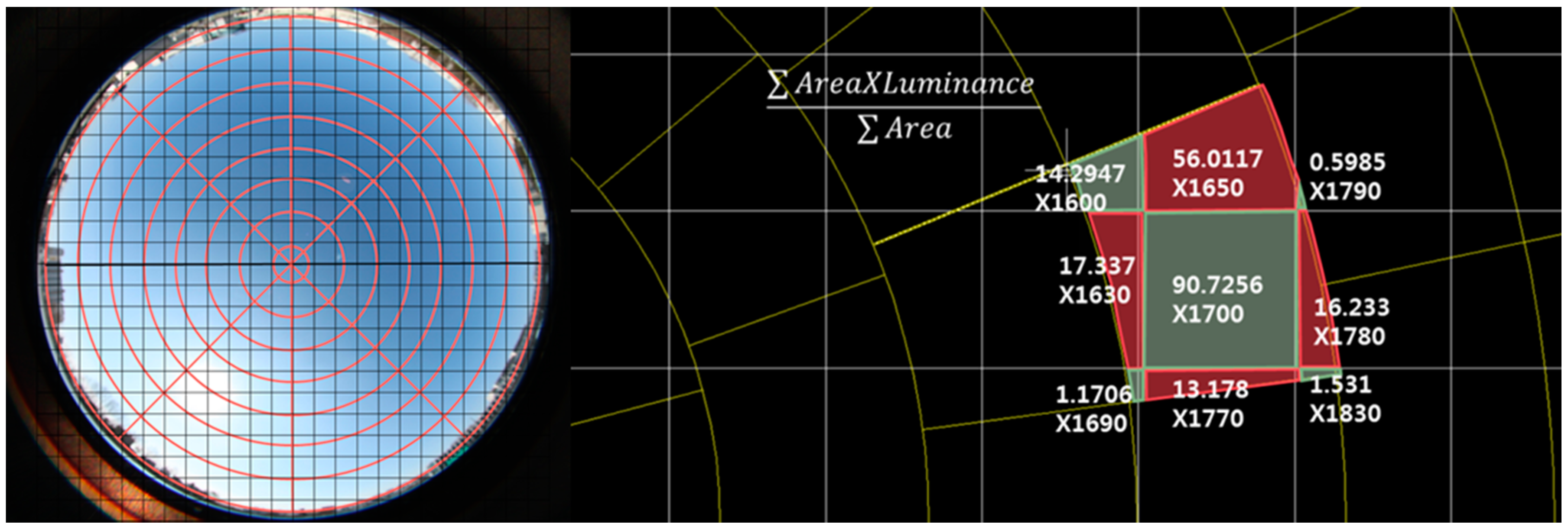
3.2.2. Analysis of Sky Luminance Distribution Using HDRI

A high dynamic range image (HDRI) includes a higher dynamic range of image between the brightest and the darkest areas [42]. The auto exposure bracketing (AEB) function of the DSLR camera with its fisheye lens can be used to obtain HDRIs. The HDRI is created and analyzed using several photographs taken at different exposure settings. While these images are photographs of the same scene, their exposures differ. The AEB function automatically changes the shutter speed or aperture, and the exposure splits into three values in the range of −2 to 2. In this research, various shutter speeds were used for three different exposure images. We also made the HDRIs using three photographs with exposures of −2, 0, and 2. In this research, these three images are combined using the Photosphere program. The screen in the Photosphere program is shown in Figure 5.
The Photosphere program is a photo editing tool that can easily produce HDRIs. After the HDRIs are created, the calibration process is absolutely necessary. In general, HDRIs are corrected by measuring the luminance of the gray target by luminance meter while simultaneously capturing the gray image in the HDRI. However, when analyzing the sky using HDRIs, calibration with a luminance meter is not appropriate [43]. Instead, it is more accurate to calculate the calibration factor using the measured illuminance value at the same level as the camera. The formula for calculating illuminance with luminance measured with HDRI is
E = 0 2 π 0 π / 2 L γ α   sin θ   cos θ   d θ   d φ
HDRI is corrected so that illuminance calculated by HDRI luminance is equal to illuminance measured at the same level as the camera.
After luminance correction with illuminance value, the vignetting effect must also be calibrated. HDRI taken with a fisheye lens is heavily influenced by the vignetting effect. The loss of luminance at the center of the image is negligible. However, the error increases towards the end of the image. We multiplied the luminance of each part of HDRI by the correction constant according to altitude angle to correct luminance loss due to vignetting effect. We measured the aperture with f/4. The vignetting effect of HDRI used in this study was calibrated with reference to Inanici [43].
With the Photosphere program, the luminance value of the selected part can be obtained by clicking or dragging the required part of the HDRI. For comparison with the luminance values of the calculation models, we need to obtain the luminance values of 145 patches defined by the azimuth angle and the altitude angle. Because we can only obtain a square shape by clicking or dragging, we can observe the luminance of the grid form contour by the Photosphere program. Therefore, it is necessary to change the grid form contour to the curved form contour.
First, it is necessary to calibrate the position of the sphere sky image taken by the CCD camera. For calibration of the position, a dome with 145 sky patches was projected on the calibration box, and the image of the dome was taken with a CCD camera. The calibration box was drawn by projecting 145 sky patches in three dimensions. Through this process, we can determine the real position of each sky patch in the HDRI in which the sphere sky was captured [21]. The process for calibration is shown in Figure 6.
Second, we need to determine the relationship of the position between the sphere shape sky contour divided into 145 segments and the grid-shaped sky contour. These two types of sky contours overlap, as shown on the left side of Figure 7. The average luminance of area of each of the 145 sky patches enclosed by the curve can then be calculated from the weighted average of the luminance of the grid contour (Figure 7, right). The luminance value obtained from the HDRI by the photosphere program is multiplied by the area created by intersection of the grid contour and the circular contour. All values for one of 145 patches are added and divided by the area of the patch. The formula is shown as follows. In HDRI, the luminance value of the portion without the image is calculated as 0.
The   luminance   value   of   one   of   the   145   patches = Σ ( Area × Luminance   of   grid   contour )   Σ Area
In summary, the luminance of 145 patches can be calculated using a grid form luminance contour, and HDRI can be used to determine the luminance contour in a grid form (Figure 8).

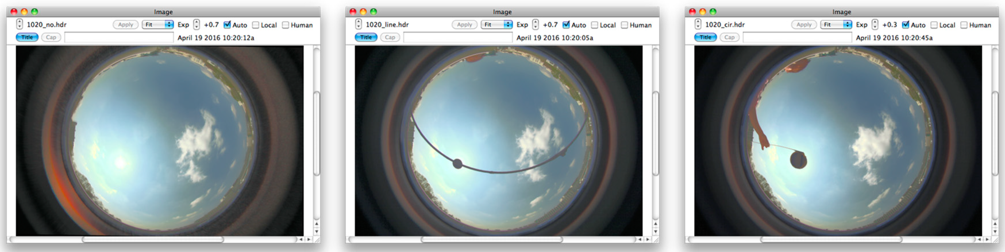
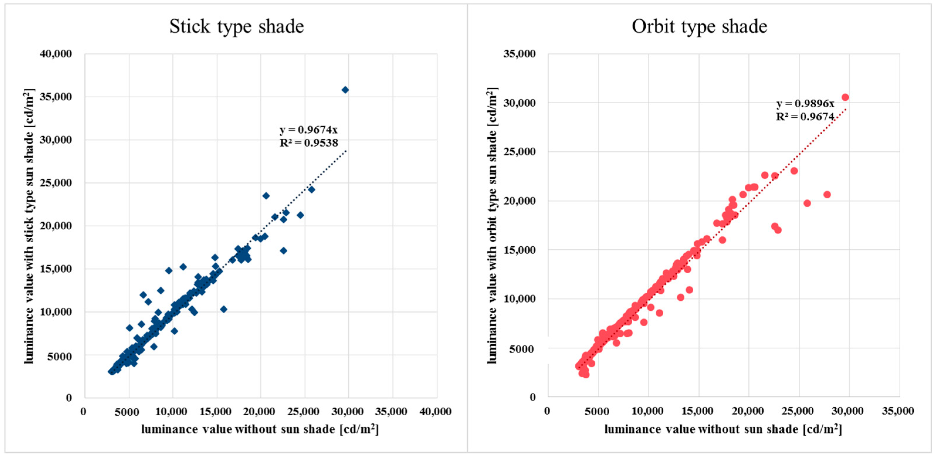
3.2.3. Analysis of Sun Shade Necessity

The most influential factor affecting sky luminance distributions is the location of the sun. In the case of an overcast sky, the sun is relatively screened by clouds, so the influence of the sun is weak. However, in the case of a clear sky, the contour of the sky patches is not clearly revealed because the difference in luminance value between the sun and the other portion of the sky is too large. Therefore, in many previous studies, the sky picture was taken after covering the sun with a sun shade (Cabrera, 2010; Shields et al., 2013). However, since the luminance of each sky patch is measured in the Photosphere analysis, it is possible to analyze the contour of the sky luminance without using the sun shade. To verify this, HDRIs both with and without the sun shade were captured and were then compared.
The HDRIs for three variables such as no sun shade, orbit type sun shade, and stick type sun shade are shown in Figure 9.
The luminance distributions shown by the grid form contour at certain times are shown in Figure 10.
When the two types of shade were installed, since the sun was covered and the luminance of the brightest part was somewhat low, the change in luminance contour was easy to see. In the case without the sun shade, the contours near the sun were difficult to identify because the luminance of the sun was much greater than the luminance of the other sky parts.
A comparison between the skies with and without the sun shade is shown in Figure 11.
When comparing the luminance values, we excluded data near the sun. The R2 of the luminance value of each part, except the sun part, is 0.95 for the stick type sun shade, and 0.97 for the orbit type sun shade. The slope (Y) of the stick type is 0.97 and that of the Orbit type is 0.99. Therefore, the HDRIs photographed without and with sun shades show similar results.

3.3. Comparison Methods

To evaluate the algorithm described above against the measured values, statistical tests were used. The R2 value indicating the agreement rate of the two values, the mean bias error (MBE), the coefficient of variation of the root mean square error (Cv(RMSE)) [44], and t-statistic [45] were used to compare the measured value with the luminance value of the calculated sky model.
The MBE is defined as
MBE = {(∑Period (S − M)interval)/(∑PeriodMinterval)} × 100
where
  • M is measured data,
  • S is simulated data.
The Cv(RMSE) is defined as
Cv(RMSEPeriod) = (RMSEPeriod/APeriod) × 100
RMSE Period = ( S M ) interval 2 N interval
APeriod = ∑PeriodMinterval/Ninterval,
where
  • Ninterval is the number of time intervals in the monitoring period.
The t-statistic is defined as
t = [ ( N 1 ) MBE 2 RMSE 2 MBE 2 ] 1 / 2

4. Results

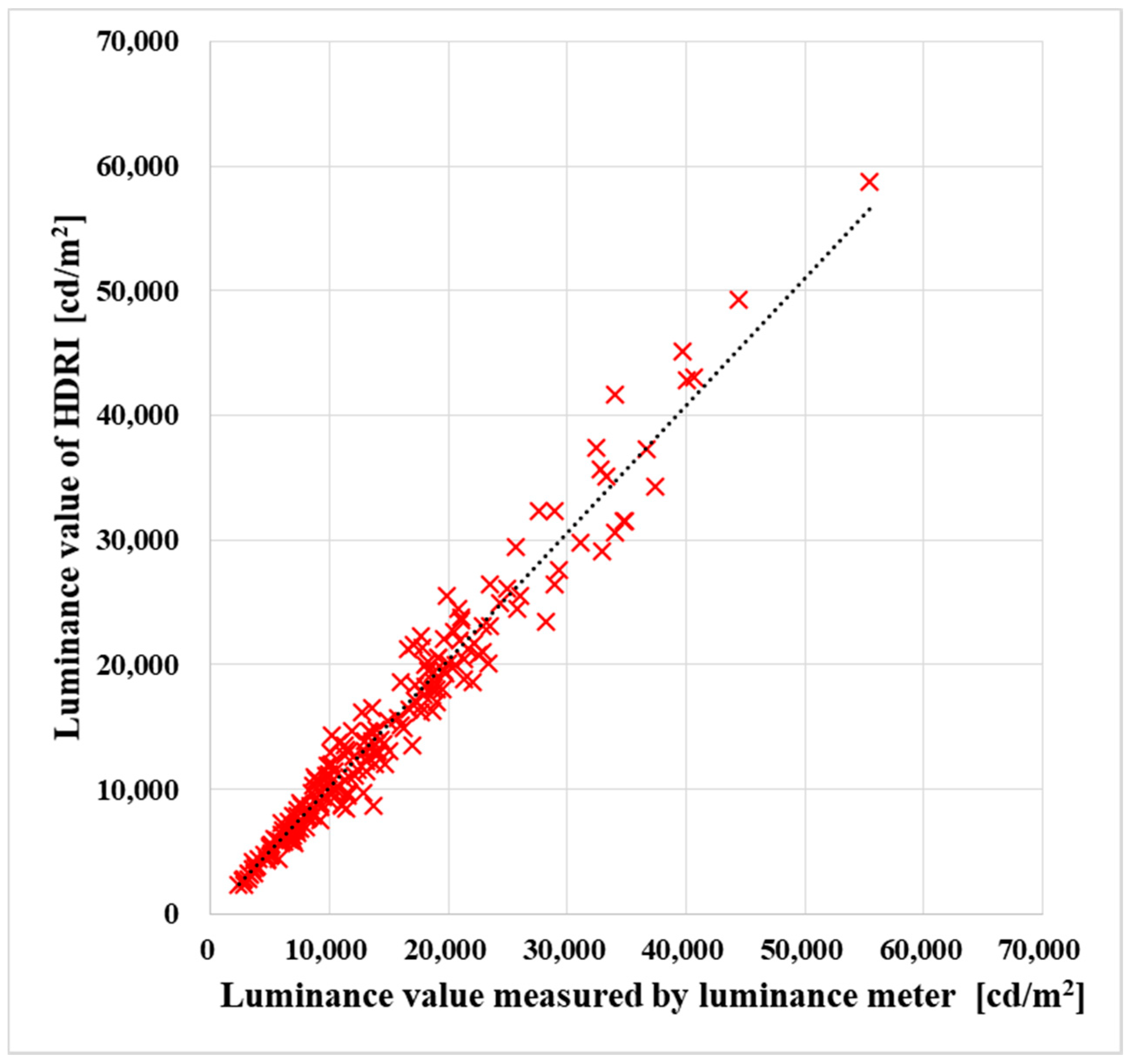
4.1. HDRI Verification Using Zenith Luminance

All HDRIs are calibrated using the horizontal illuminance value, which is measured at the same level as the CCD camera. Figure 12 shows the agreement of the two zenith luminance values obtained with the two methods (one method is the data measured with a spot luminance meter, while the other method is the data obtained from the calibrated HDRI).
The error rates are shown in Table 4.
MBE and Cv(RMSE) of the two values were 0.9% and 12.1%, respectively, with R2 of 0.99. Therefore, the agreement of the two values was high. Thus, luminance values of measured HDRIs are then verified.

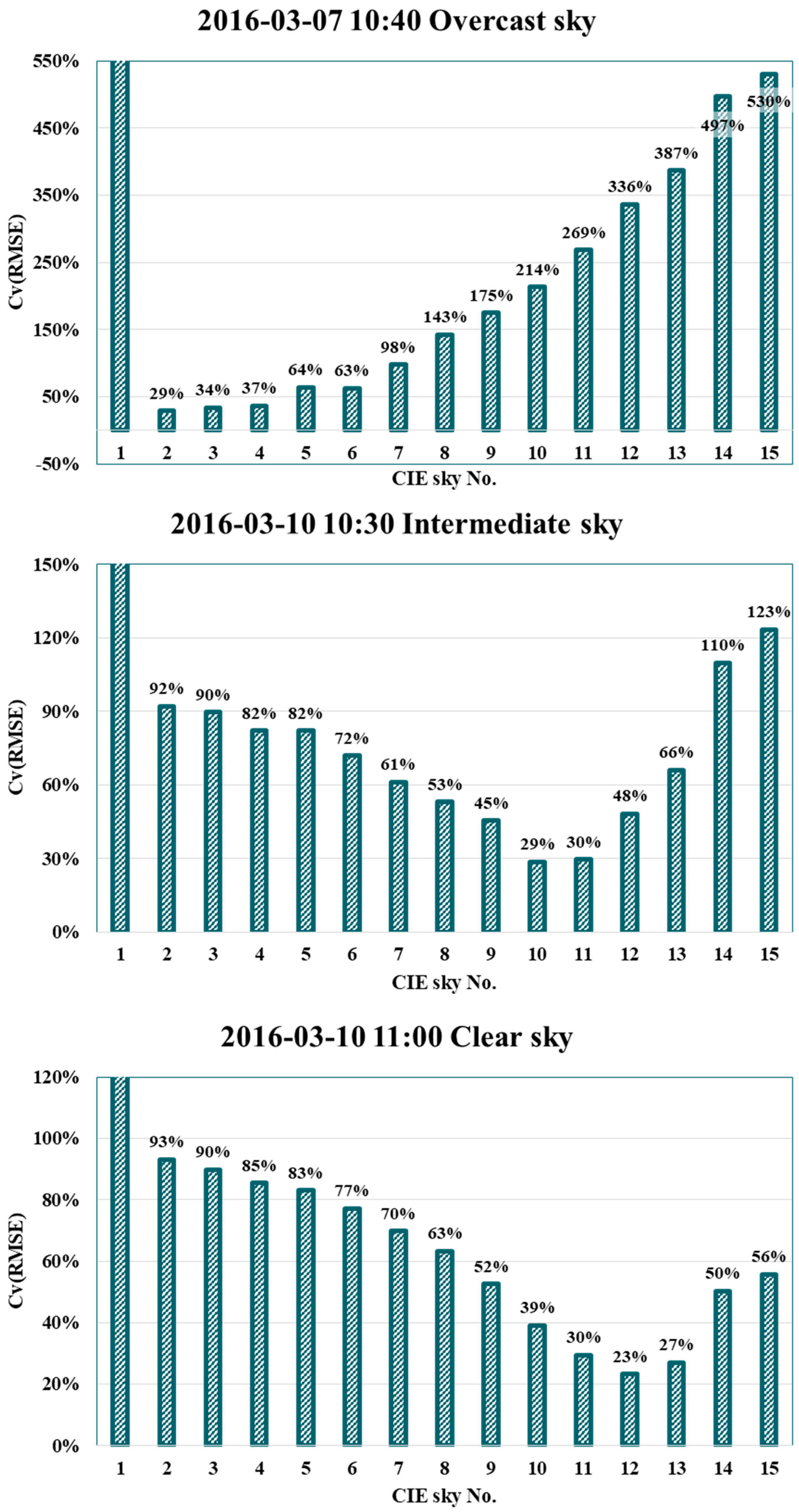
4.2. Calculation Method of CIE Standard Sky Model

The CIE standard sky model does not provide clear criteria for the selection of sky types [15]. The CIE guide [25] recommends a method of calculating the value of the ratio of the zenith luminance to the horizontal diffuse illuminance, Lz/EdH. However, this recommended criterion is only valid when solar altitude is lower than 30 degrees. In our study, we compared luminance values of all 145 sky patches and then selected a sky number with a minimum Cv(RMSE) value. This is because there is no limit to solar altitude. It is possible to utilize the CIE standard sky model as an important indicator for analyzing HDRI since the overall luminance is compared. Representative examples for Clear sky, Intermediate sky, and Overcast sky were selected for the analysis of selection method. Representative time of clear sky was 11:00 am on March 10. That of intermediate sky was 10:30 am on March 10 and that of overcast sky was 10:40 am on March 7. The Cv(RMSE) values calculated by comparing the data of each representative time with CIE standard sky are shown in Figure 13.
The sky at 11:00 am on March 10 was determined as the No. 12 Clear sky in the CIE standard general sky model. In comparison with clear sky as a whole, the error was low. However, the error tended to increase in overcast sky. The sky at 10:30 am on March 10 was identified as the No. 10 Intermediate sky. The overcast sky at 10:40 am on March 7 was identified as the No. 2 Overcast sky. The tendency of error in intermediate sky and overcast sky was similar to the tendency of clear sky error. The sky determined by intermediate sky has a larger error as it approaches clear sky and overcast sky. The sky determined as overcast sky has a larger error as it approaches clear sky. All HDRIs selected corresponding CIE standard sky model numbers in the same way.
When we analyzed the overcast sky case, even though No. 1 sky is classified as an overcast sky, the No. 1 overcast sky shows weak agreement with the measured overcast data. This is because the No. 1 overcast sky is an ideal sky in which the luminance distribution from the zenith to the horizontal plane is gradually decreased. However, the actual overcast sky luminance cannot be distributed in the same way as the ideal overcast sky because of the sun and the variation in the thickness of the cloud. Therefore, even though the measured sky was overcast sky, the Cv(RMSE) of the No. 1 CIE standard sky was high.

4.3. Analysis of Sky Luminance Distribution Calculation Method

First, we checked the data classified as No. 3 overcast sky in the CIE standard sky model (Figure 14).
A graph comparing the luminance values of each part of HDRI with three types of sky models (Perez model, Igawa model, and CIE standard sky model) is shown in the center of Figure 14: the upper side shows the March data and, the lower side shows the July data. Because both March and July data were classified as overcast sky, the luminance distributions in the three sky models gradually decreased from zenith to the horizontal plane. The values of diffuse irradiance were not significantly different from the values of global irradiance. As a result, both the Perez model and the Igawa model were calculated as Overcast sky. The diffuse irradiance of the two skies was (186.9 and 139.8) W/m2, respectively. Overcast sky is affected by cloud. Therefore, if the cloud is uneven, the empirical calculation model and the actual measurement model will have large errors. Therefore, in March and July, the luminance graph of HDRI showed a rule-free form. The error was larger in July than in March, which can be interpreted as the difference in cloud thickness and evenness.
Figure 15 shows the results of the analyzed March and July data, classified as No. 10 and No. 8 intermediate CIE standard sky, respectively.
As can be seen from the photo on the left side of Figure 15, the clouds cover the sky with a relatively constant thickness and the position of the sun can be easily determined because the clouds are relatively thin. Both data (March, July) showed a high agreement rate with the calculated sky model, but the data of July showed a slightly higher error than the data of March as shown in the middle area of Figure 15. In March, the luminance value calculated by the Igawa model was generally high. On the other hand, in July, the calculation of the Perez model was generally high.
Figure 16 shows the results of the analyzed March and July data, classified as No. 12 and No. 13 CIE standard sky.
The graphs comparing the luminance values of HDRI with the calculated sky models are shown in the center of Figure 16. These two data of March and July show that the solar altitude in July was higher than in March. In July, because of the high solar altitude, the amount of solar irradiance reaching the earth surface is high. As can be seen from the data of July, even though the diffuse irradiance value was relatively high, it was judged to be a clear sky by the CIE sky model which compares the entire sky. However, the Perez model, in which the ratio of diffuse irradiance to global irradiance is important, was identified as category 7, and the Igawa model was also identified as near clear sky. CIE Sky is a result of comparing the whole sky, so it reflects more realistic sky conditions. On the other hand, the March data is classified as clear sky in all three types of sky models (Perez model, Igawa model, and CIE standard sky model). As can be seen in the center of Figure 16, the correlation rate of the March data is higher than that of the July data.
Figure 17 shows the R2, MBE, and Cv(RMSE) values of all sky luminance distributions measured. The values are shown in Table 5.
The R2 in the CIE standard sky was 0.93, that in the Igawa model was 0.91, and that in the Perez model was 0.83 with the measured data. The MBE value is an indicator of whether the calculated value is higher or lower than the measured value. In the CIE model and the Perez model, the MBE was positive, which means that it was calculated to be higher than the measured value. In the Igawa model, the MBE value was calculated as a negative value, which means that the Igawa model was calculated to be lower than the measured value. For the Cv(RMSE) value, the Perez model has the highest value of 62.2%, and the CIE standard sky model has the lowest value of 36.4% when compared with HDRI. The CIE sky model has the advantage of selecting the sky with the lowest Cv(RMSE) among the 15 categories, but CIE standard sky model has few options. The Perez model and the Igawa model must calculate each luminance value, but the luminance can be calculated for each situation. The Perez model and CIE standard sky model showed higher Cv(RMSE) in July than in March. The Igawa model showed no significant difference in Cv(RMSE) between March and July. Figure 17 and Table 5 show results calculated for all luminance of the sky patch. The errors were large due to irregular cloud conditions (intermediate sky, overcast sky) and buildings taken together near the horizon.
In order to determine why the March and July data differ, we compared the CIE standard sky model number with the sky clearness by the Perez model and the sky index by the Igawa model [46]. The comparison is shown in the graph in Figure 18.
Data shown in the box drawn with a red dotted line in Figure 18 indicate that the sky condition is the same as the CIE standard sky model. First, we compared sky clearness of the Perez model with the sky number of the CIE standard sky model in March and July. In the March data, in a case in which the CIE standard sky No. is 1 to 5 (overcast sky), the category based on sky clearness is mainly in the range of 1 to 2. When the CIE standard sky No. is from 6 to 10 (intermediate sky), the category based on sky clearness is mostly in the range of from 3 to 6. When the CIE standard sky No. is from 11 to 15 (clear sky), the category based on the sky clearness was mostly distributed as 7 or 8. This means that the criteria of the CIE standard sky and Perez models produce similar results for the March data. However, the data of July differed to that of March. The data for July were more often not displayed in the box drawn with a red dotted line than in March. In March, 66% of HDRIs evaluated as clear sky in the CIE standard sky model were rated as clear sky in the Perez model. However, in July, 23% of HDRIs evaluated as clear sky with the CIE standard sky model were identified as clear sky in the Perez model while the remaining 77% were identified as intermediate sky. Since the CIE model is selected by comparing the luminance of the entire sky, the judgment by the CIE model is more realistic. This result means that when analyzing the same sky, the Perez model is often closer to overcast sky than the CIE standard sky model especially in July.
The correlation between the Igawa model and the CIE standard sky model was higher than that between the Perez model and the CIE standard sky model. For March data, when the CIE standard sky No. was 1 to 5 (overcast sky), the Igawa model was also mostly classified as overcast sky. When the CIE standard sky No. was 6 to 10 (intermediate sky), the sky index often indicated intermediate sky. When the CIE standard sky No. was 11 to 15 (clear sky), the sky index often indicated clear sky. In the Igawa model, data of July were not more consistent with the CIE standard sky model than data of March. However the difference was not significant compared with the Perez model.
Data for March showed 71% of the Perez model and 87% of the Igawa model in a box drawn with a red dotted line. However, in July, only 56% of the Perez model and 76% of the Igawa model were in the red dashed box. When the measured HDRI was classified according to sky condition category, data classified by the criteria of the CIE standard sky model was more similar to the data classified by the Igawa model than the Perez model. The agreement of the CIE standard sky model with the sky conditions of the Perez model and the Igawa model was lower in July than in that in March.

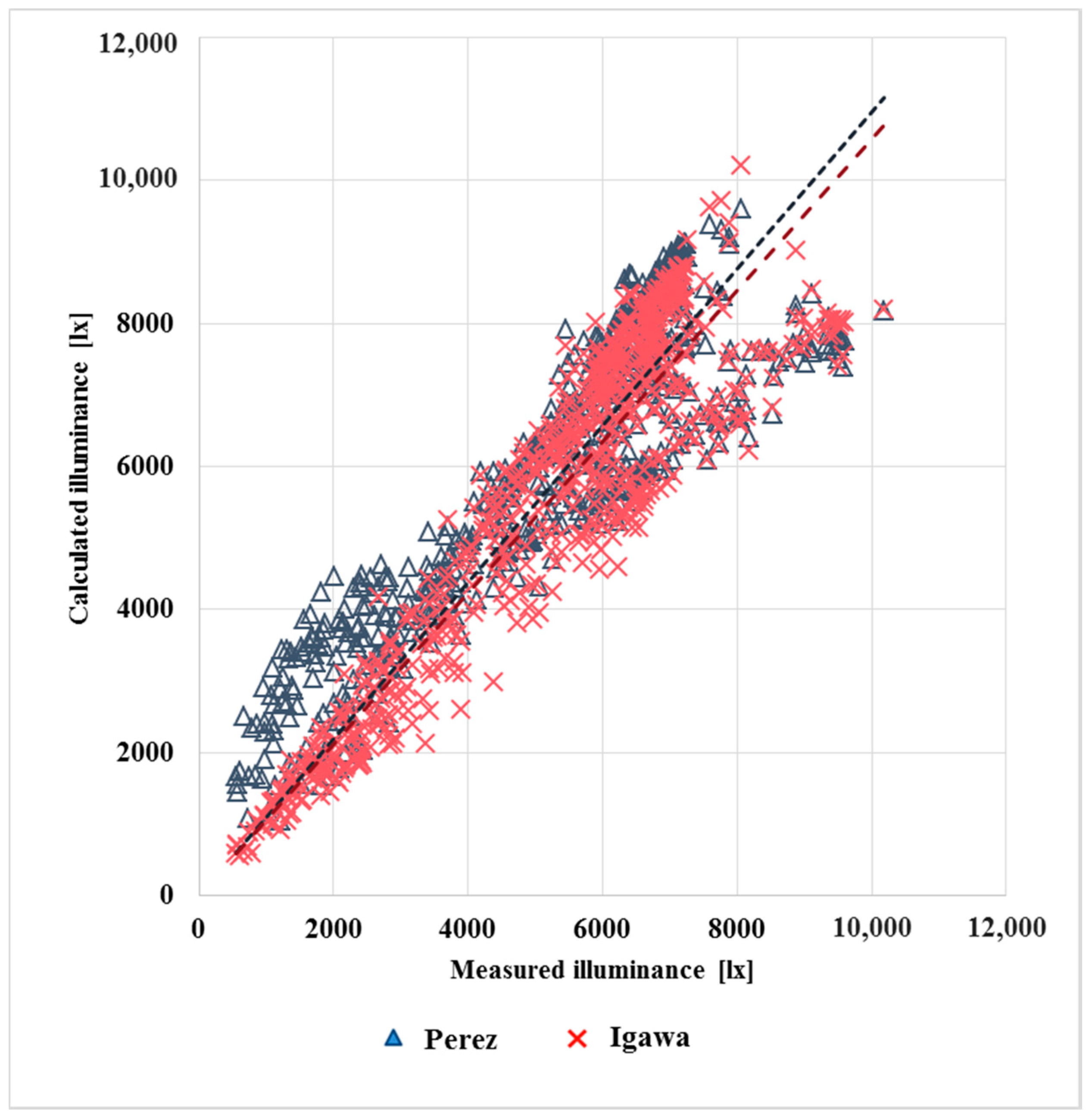
4.4. Analysis of Calculated Vertical Illuminances

Among the three sky models, the vertical surface illuminance was calculated using the Perez model and the Igawa model. Because the CIE model does not provide general criteria to select sky categories independently of the measured data of luminance, it cannot be used as a general input when predicting illuminance [27]. We compared the calculated vertical illuminance with the measured values. The comparison is shown in a graph in Figure 19.
The error rate is shown in Table 6.
Regarding the difference in vertical illuminance between measured values and calculated values using the Perez model, the following results were obtained: MBE, 11%; Cv(RMSE), 20%; R2, 0.97; t-stat, 0.00031. In the Igawa model, MBE was 3%, Cv(RMSE) was 14%, R2 was 0.99 and t-stat was 0.00014. For illuminance on a vertical surface calculated using the luminance value of the sky luminance distribution models, the Igawa model had a lower error rate than the Perez model. Since the global illuminance on a vertical surface is calculated by adding the diffuse component and the direct component, the results are influenced by the direct component because the direct component is calculated in the same algorithm, regardless of the calculation model. To compare the difference between the Perez model and the Igawa model used as variables in the calculation algorithm, it is necessary to compare only diffuse illuminance which is calculated by another algorithm. For comparison of the vertical illuminance calculated by different sky luminance distribution algorithms, except for the direct component, only overcast sky was analyzed. The graph is shown in Figure 20.
The error is shown in Table 7.
When the Perez model was applied, the calculated MBE was 86%, Cv(RMSE) was 103%, R2 was 0.72, and t-stat was 0.00082. When the Igawa model was applied, MBE was 6%, Cv(RMSE) was 22%, R2 was 1.00, and t-stat was 0.00027. In case of overcast sky with low influence of direct component, the error rate of Perez model was bigger than that in total sky condition. The error calculated by the Igawa model compared with the vertical illuminance measured in Korea was lower than that of the Perez model.

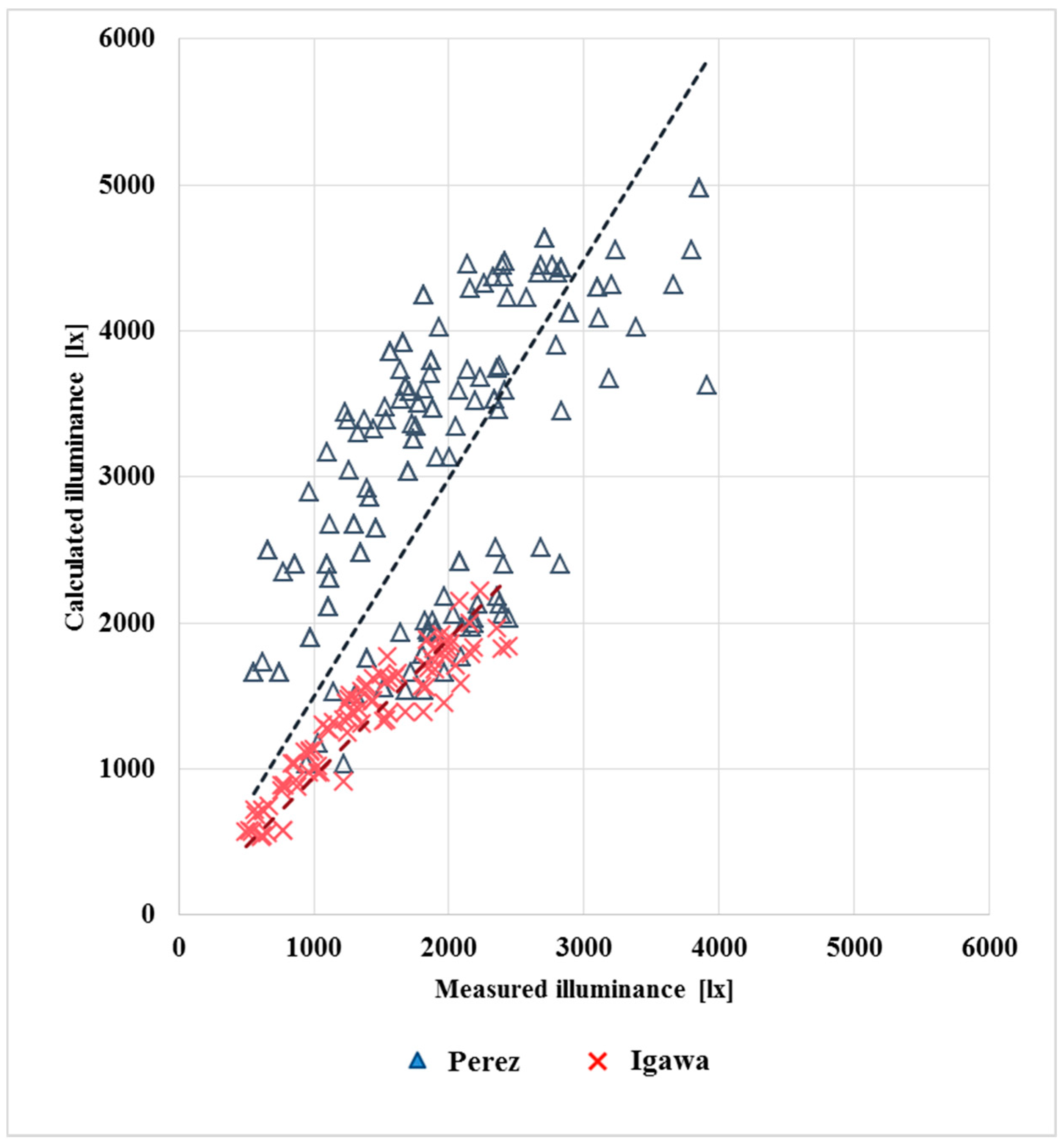
4.5. Analysis of Calculated Interior Illuminance

Using the DeLight algorithm, the horizontal illuminance of the daylight entering a room was calculated and compared with the measured illuminance value. Figure 21 shows a comparison of the interior horizontal illuminances.
First, we compared the results in all sky conditions. When the indoor illuminance was calculated with the Perez model, MBE was 13%, and Cv(RMSE) was 22%; when using the Igawa model, MBE was 6%, and Cv(RMSE) was 18%. This value is a comparison of values containing the direct component. Comparisons of diffuse components are important to find models with lower error compared to measured values in Korea between Perez and Igawa models. Therefore, we analyzed the error of overcast sky without the direct component. The graph comparing only overcast sky is shown in Figure 22.
The error rate is shown in Table 9.
To analyze calculation results of the diffuse component, only overcast sky was arranged. Diffuse component values of the Perez model were higher than measured values in most results. Compared with measured values in overcast sky, the Perez model showed high error while the Igawa model was a more suitable sky luminance distribution model for Korea.

5. Discussion and Conclusions

This study proposes a method to analyze the sky conditions using HDRI with a CCD camera. The sky data obtained by analyzing HDRI with a CCD camera was compared with the three sky analysis models of the Perez model, Igawa model and CIE standard sky model, and the vertical surface illuminance was calculated. Then, we calculated the indoor illuminance using the calculated vertical surface illuminance and compared it with the measured value. This study focused on diffuse components, one of the major causes of error, rather than direct components. The conclusions drawn are as follows.
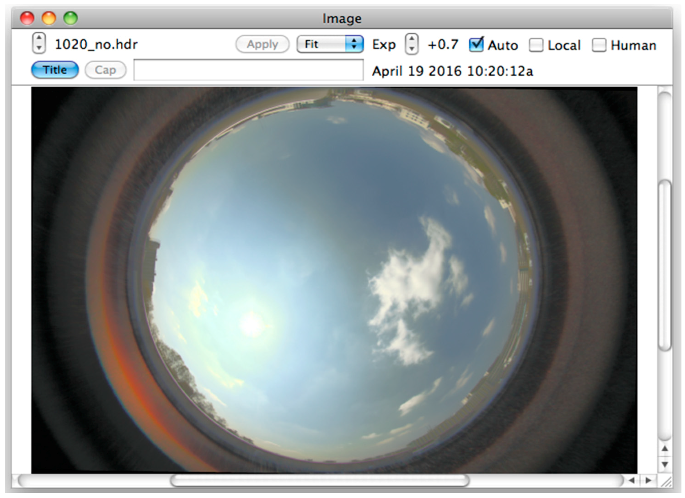
  • Since the luminance near the sun is relatively large in the sky luminance measurement using a CCD camera, it may be necessary to cover the sun or use a filter to measure it. HDRI with a sun shade and HDRI without a sun shade were compared with each other. We used HDRI without a sun shade for the analysis because the error was not large.
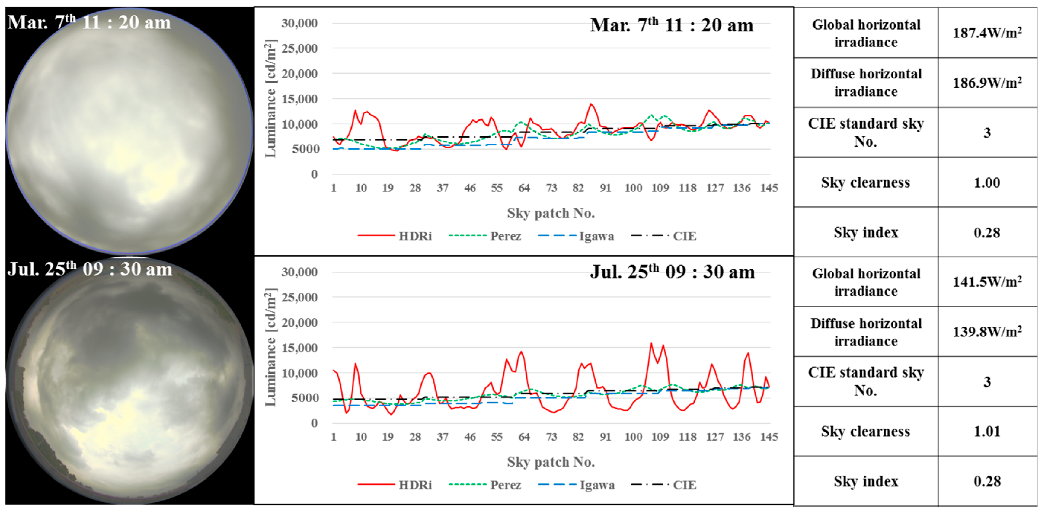
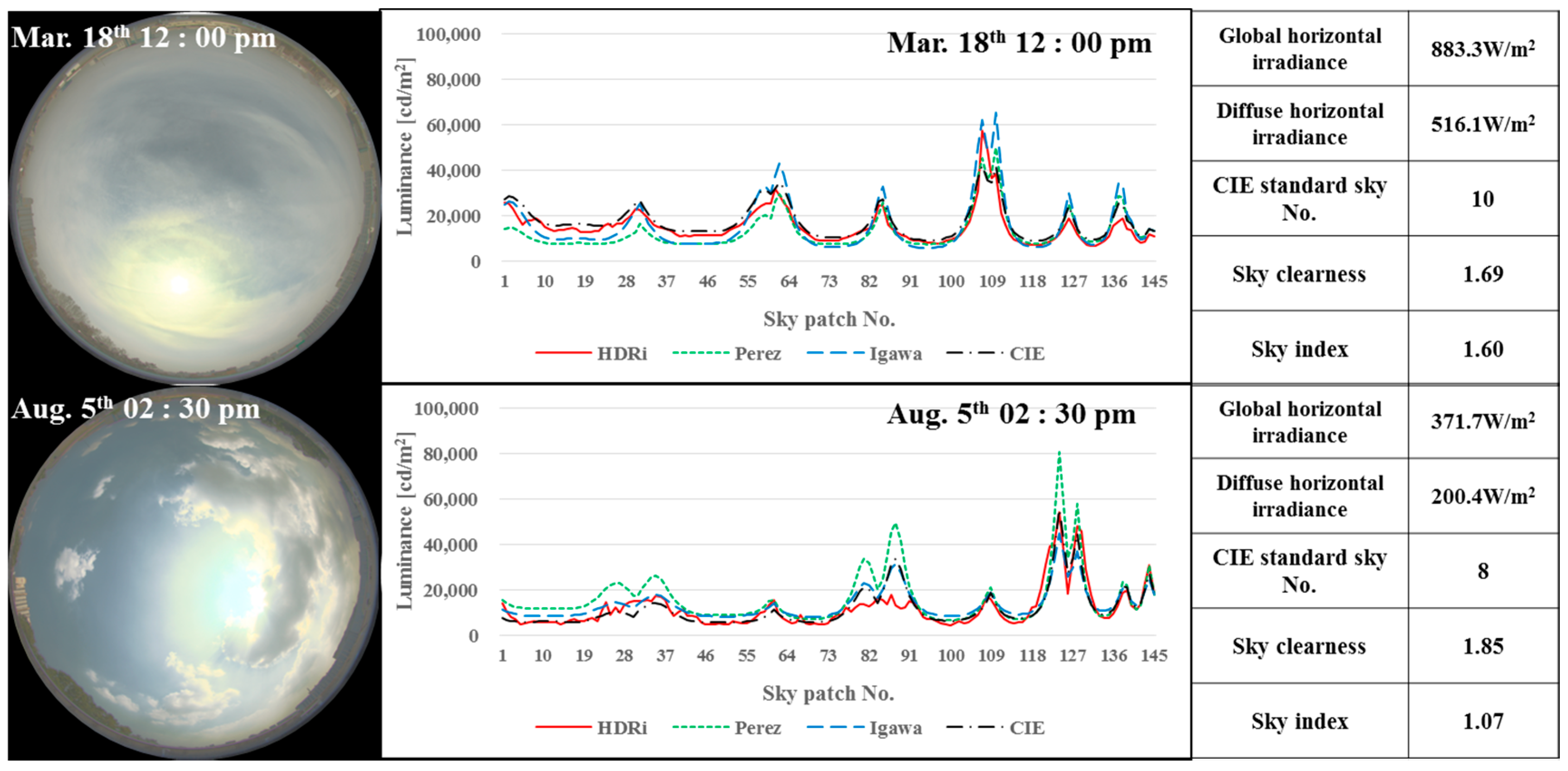
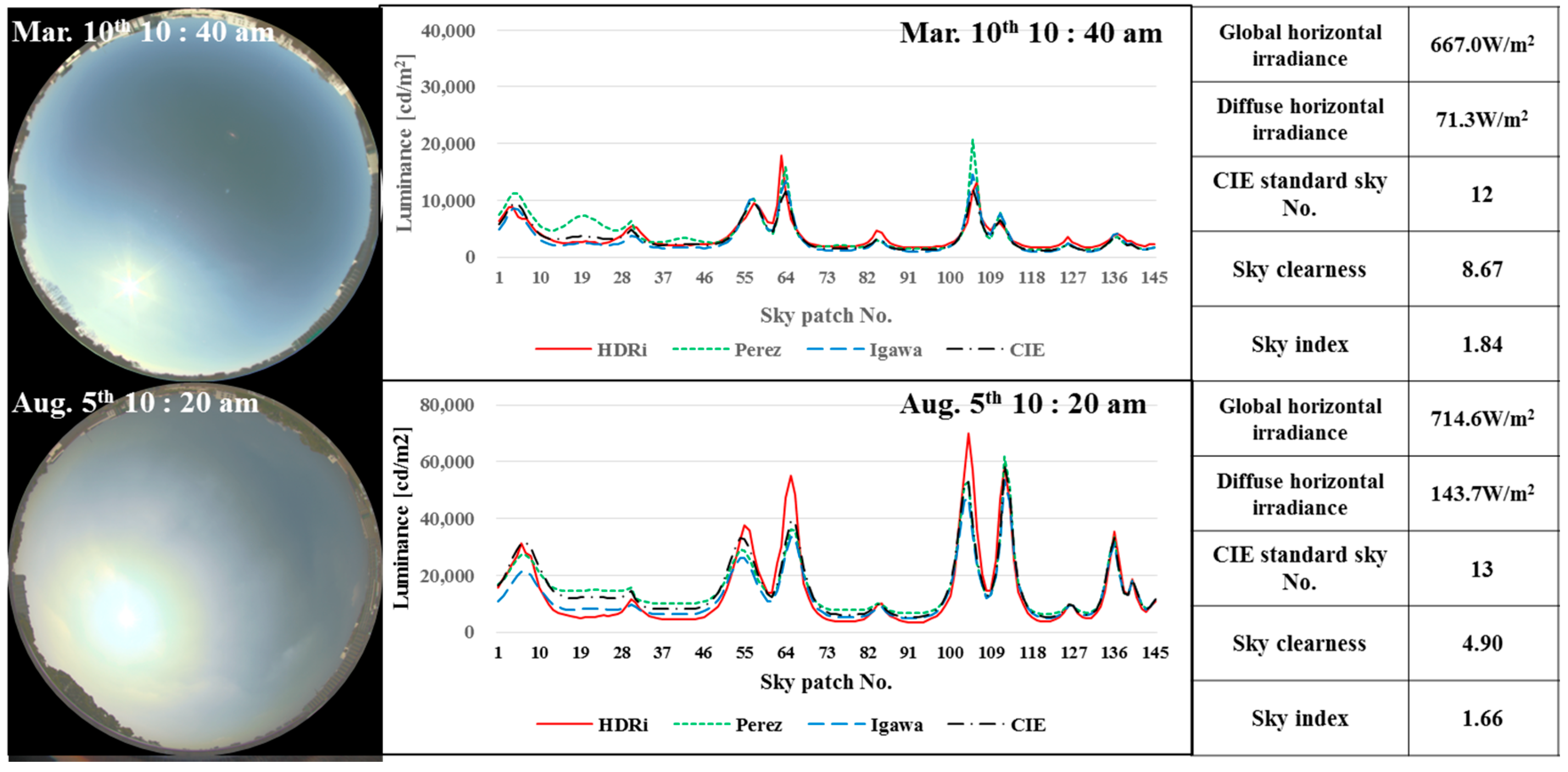
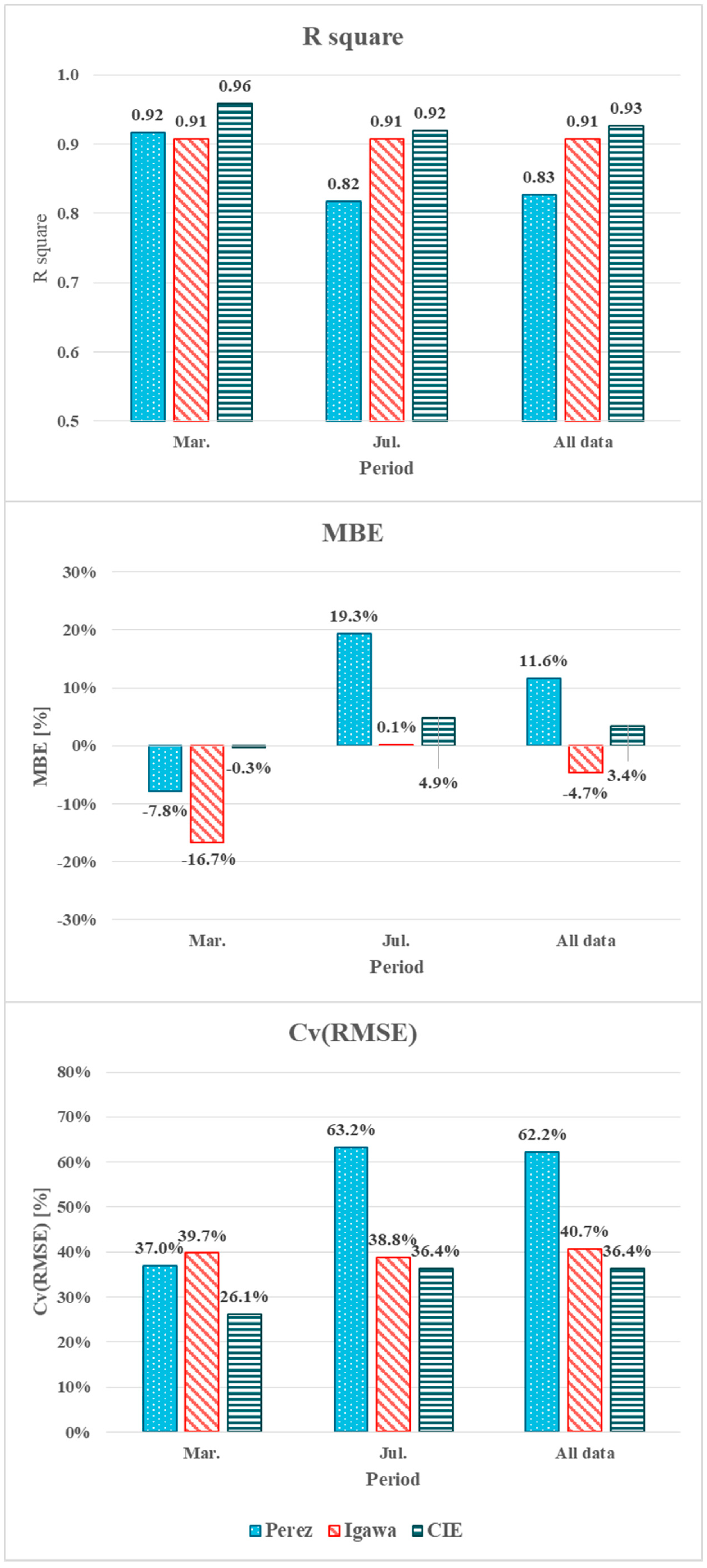
  • When comparing March and July measurements with the sky luminance distribution model, the Igawa sky luminance distribution model and the Perez sky luminance distribution model both had higher error rates in July than in March. High solar altitude is known to increase the error of prediction results. Such result might be due to the high solar altitude in July. However, the result when meridian altitude was lower than 45.5 degrees was not verified by measurement. Therefore, additional verification is required when the meridian altitude is lower than 45.5 degrees.
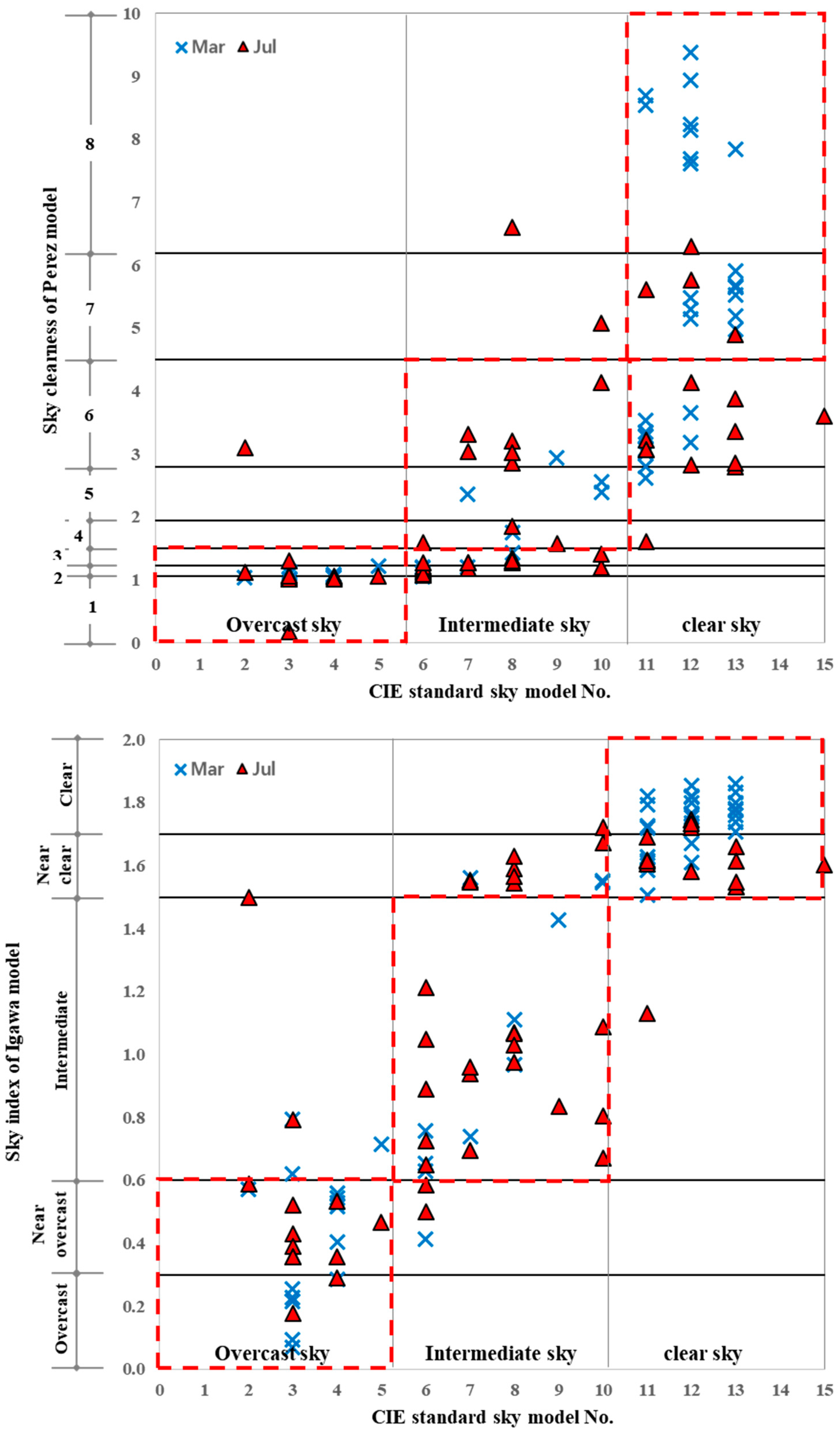
  • When intermediate skies based on the CIE standard sky model were analyzed, most sky conditions in March were calculated as intermediate sky in the Perez model and the Igawa model. However, in July, when the solar altitude was high, the CIE standard sky model was often closer to a clear sky than the Perez or Igawa model. The Igawa model was often closer to a clear sky than the Perez model.
  • For R2, MBE, and Cv(RMSE) analysis, the CIE standard sky model showed the highest agreement rate and the lowest error rate. Between the Perez model and Igawa model, the Igawa model showed a lower error rate when HDRI was compared. However, the CIE standard sky model could only be used for calculation by knowing the luminance of the sky as a whole. Therefore, the Igawa model is the most suitable option for predicting sky luminance distribution with measured solar irradiance.
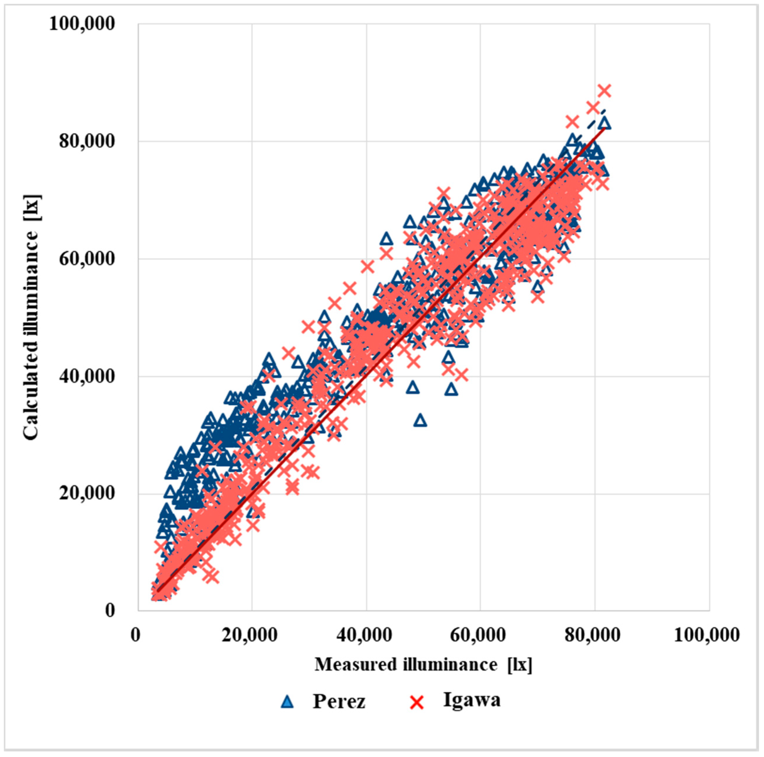
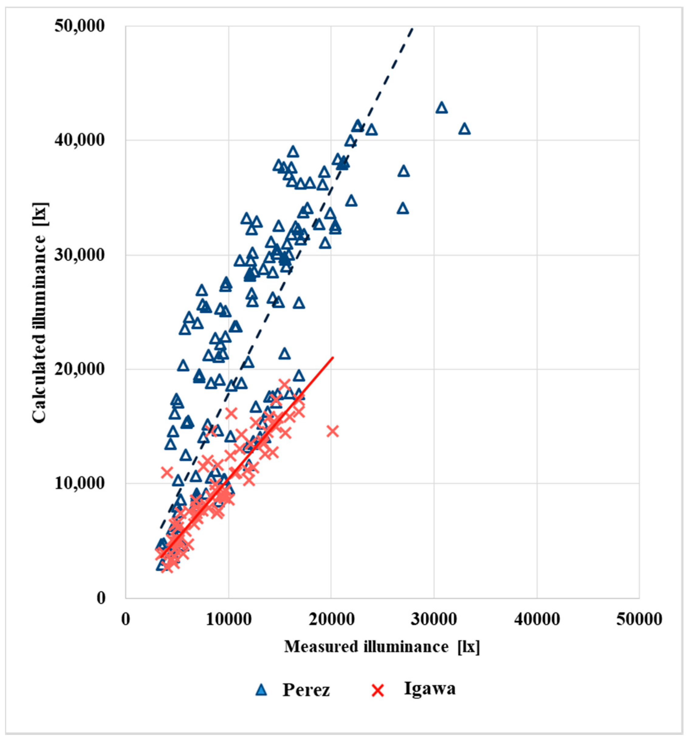
  • Perez and Igawa models were used to calculate the vertical illuminance and internal illuminance. When comparing all sky conditions, the error between the Perez model and Igawa model did not differ greatly. This is due to the influence of the direct illuminance component. Because only diffuse illuminance was obtained by luminance distributions of the sky model, only overcast sky was compared. In vertical illuminance calculation, the error rate of the Igawa model was lower than that of the Perez model. This trend is consistent when comparing the measured HDRI to calculated sky model luminance distribution.
  • Additional errors in sky luminance distribution might be due to the simplified measurement method, especially when it is near the horizontal plane because buildings could interfere with the analysis by being photographed in the HDRI.
  • The Igawa model is better to use than the Perez model for diffuse illuminance calculations. The formula for calculating the vertical and the interior illuminance from sky luminance distributions continuously needs to be verified with more data. The CCD camera, which can measure in a relatively easy way, can help to collect this data.

Author Contributions

S.-I.Y. performed the measurement and data analysis, and wrote this paper based on the obtained results. K.-S.K. led and supervised this study. All of the authors have contributed for collecting ideas and concepts presented in the paper.

Acknowledgments

This work was supported by the National Research Foundation of Korea(NRF) grant funded by the Korea government(MSIP) (No. 2017R1D1A1B03028205).

Conflicts of Interest

The authors declare no conflict of interest.

References

  1. Alrubaih, M.S.; Zain, M.F.M.; Alghoul, M.A.; Ibrahim, N.L.N.; Shameri, M.A.; Elayeb, O. Research and development on aspects of daylighting fundamentals. Renew. Sustain. Energy Rev. 2013, 21, 494–505. [Google Scholar] [CrossRef]
  2. Doulos, L.T.; Tsangrassoulis, A.; Topalis, F.V. Multi-criteria decision analysis to select the optimum position and proper field of view of a photosensor. Energy Convers. Manag. 2014, 86, 1069–1077. [Google Scholar] [CrossRef]
  3. Doulos, L.T.; Tsangrassoulis, A.; Kontaxis, P.A.; Kontadakis, A.; Topalis, F.V. Harvesting daylight with LED or T5 fluorescent lamps? The role of dimming. Energy Build. 2017, 140, 336–347. [Google Scholar] [CrossRef]
  4. Doulos, L.T.; Tsangrassoulis, A.; Topalis, F. Quantifying energy savings in daylight responsive systems: The role of dimming electronic ballasts. Energy Build. 2008, 40, 36–50. [Google Scholar] [CrossRef]
  5. Bellia, L.; Fragliasso, F.; Pedace, A. Evaluation of daylight availability for energy savings. J. Daylight. 2015, 2, 12–20. [Google Scholar] [CrossRef]
  6. Perez, R.; Seals, R.; Mechalsky, J. All-weather model for sky luminance distribution—Preliminary configuration and validation. Sol. Energy 1993, 50, 235–245. [Google Scholar] [CrossRef]
  7. Kittler, R.; Perez, R.; Darula, S. A new generation of sky standards. In Proceedings of the 8th European Lighting Conference (LUX Europa 1997), Amsterdam, The Netherlands, 11–14 May 1997; pp. 359–373. [Google Scholar]
  8. Igawa, N.; Koga, Y.; Matsuzawa, T.; Nakamura, H. Models of sky radiance distribution and sky luminance distribution. Sol. Energy 2004, 77, 137–157. [Google Scholar] [CrossRef]
  9. Brunger, A.P.; Hooper, F.C. Anisotropic sky radiance model based on narrow field of view measurements of shortwave radiance. Sol. Energy 1993, 51, 53–64. [Google Scholar] [CrossRef]
  10. Li, D.H.W.; Lau, C.C.S.; Lam, J.C. Evaluation of overcast-sky luminance models against measured Hong Kong data. Appl. Energy 2001, 70, 321–331. [Google Scholar] [CrossRef]
  11. Chirarattananon, S.; Chaiwiwatworakul, P. Distributions of sky luminance and radiance of North Bangkok under standard distributions. Renew. Energy 2007, 32, 1328–1345. [Google Scholar] [CrossRef]
  12. Markou, M.T.; Bartzokas, A.; Kambezidis, H.D. A new statistical methodology for classification of sky luminance distributions based on scan data. Atmos. Res. 2007, 86, 261–277. [Google Scholar] [CrossRef]
  13. Wittkopf, S.K.; Soon, L.K. Analysing sky luminance scans and predicting frequent sky patterns in Singapore. Light. Res. Technol. 2007, 39, 31–51. [Google Scholar] [CrossRef]
  14. Torres, J.L.; Blas, M.; Garcı’a, A.; Gracia, A.; Francisco, A. Sky luminance distribution in Pamplona (Spain) during the summer period. J. Atmos. Sol.-Terr. Phys. 2010, 72, 382–388. [Google Scholar] [CrossRef]
  15. Ferraro, V.; Mele, M.; Marinelli, V. Sky luminance measurements and comparisons with calculation models. J. Atmos. Sol.-Terr. Phys. 2011, 73, 1780–1789. [Google Scholar] [CrossRef]
  16. Ferraro, V.; Mele, M.; Marinelli, V. Analysis of sky luminance experimental data and comparison with calculation methods. Energy 2012, 37, 287–298. [Google Scholar] [CrossRef]
  17. Chauvin, R.; Nou, J.; Thil, S.; Grieu, S. Modelling the clear-sky intensity distribution using a sky imager. Sol. Energy 2015, 119, 1–17. [Google Scholar] [CrossRef]
  18. Li, D.H.W.; Lau, C.C.S.; Lam, J.C. Predicting daylight illuminance on inclined surfaces using sky luminance data. Energy 2005, 30, 1649–1665. [Google Scholar] [CrossRef]
  19. Li, D.H.W.; Cheung, G.H.W.; Cheung, K.L. Evaluation of Simplified Procedure for Indoor Daylight Illuminance Determination against Data in Scale Model Measurements. Indoor Built Environ. 2006, 15, 213–223. [Google Scholar] [CrossRef]
  20. CIE-Commision International de l’Eclairage. Spatial Distribution of Daylight––CIE Standard General Sky; International Commission on Illumination (CIE): Vienna, Austria, 2003. [Google Scholar]
  21. Pfster, G.; McKenzie, R.L.; Liley, J.B.; Thomas, A.; Forgan, B.W.; Long, C.N. Cloud Coverage Based on All-Sky Imaging and Its Impact on Surface Solar Irradiance. J. Appl. Meteorol. 2003, 42, 1421–1434. [Google Scholar] [CrossRef]
  22. Inman, R.H.; Pedro, H.T.C.; Coimbra, C.F.M. Solar forecasting methods for renewable energy integration. Prog. Energy Combust. Sci. 2013, 39, 535–576. [Google Scholar] [CrossRef]
  23. Kittler, R.; Darula, S. Perez, R. Advantages of new sky standards: More realistic modelling of daylight conditions in energy and environmental studies. Int. J. Energy Environ. Econ. 1999, 8, 65–71. [Google Scholar]
  24. Tregenza, PR. Analysing sky luminance scans to obtain frequency distributions of CIE Standard General Skies. Light. Res. Technol. 2004, 36, 271–281. [Google Scholar] [CrossRef]
  25. Darula, S.; Kittler, R. CIE general sky standard defining luminance distributions. In Proceedings of the 2002 Bi-annual IBPSA Conference, Montreal, QC, Canada, 12–13 September 2002; pp. 1–8. [Google Scholar]
  26. International Standardisation Organisation (ISO). Spatial Distribution of Daylight: CIE Standard General Sky; ISO Standard 15469:2004; CIE: Vienna, Austria, 2003. [Google Scholar]
  27. Ferraro, V.; Marinelli, V.; Mele, M. A method for selecting the CIE standard general sky model with regard to calculating luminance distributions. J. Atmos. Sol.-Terr. Phys. 2013, 95, 59–64. [Google Scholar] [CrossRef]
  28. Li, D.H.W.; Tang, H.L. Standard skies classification in Hong Kong. J. Atmos. Sol.-Terr. Phys. 2008, 70, 1222–1230. [Google Scholar] [CrossRef]
  29. Kasten, F.; Young, A. Revised optical air mass tables and approximation formula. Appl. Opt. 1989, 28, 4735–4738. [Google Scholar] [CrossRef] [PubMed]
  30. Vartiainen, E. Daylight modelling with the simulation tool DeLight. In Technical Report TKK-F-A799; Helsinki University of Technology: Espoo, Finland, 2000; pp. 76–85. [Google Scholar]
  31. De Rosa, A.; Ferraro, V.; Kaliakatsos, D.; Marinelli, V. Simplified correlations of global, direct and diffuse luminous efficacy on horizontal and vertical surfaces. Energy Build. 2008, 40, 1991–2001. [Google Scholar] [CrossRef]
  32. Gillette, G.; Pierpoint, W.; Treado, S. A general illuminance model for daylight availability. J. Illum. Eng. Soc. 1984, 13, 330–340. [Google Scholar] [CrossRef]
  33. Darula, S.; Kittler, R.; Gueymard, C.A. Reference luminous solar constant and solar luminance for illuminance calculations. Sol. Energy 2005, 79, 559–565. [Google Scholar] [CrossRef]
  34. Navvab, M.; Karayel, M.; Ne’eman, E.; Selkowitz, S. Analysis of atmospheric turbidity for daylight calculations. Energy Build. 1984, 6, 293–303. [Google Scholar] [CrossRef]
  35. Tregenza, P.R. Mean daylight illuminance in rooms facing sunlit streets. Build. Environ. 1995, 30, 83–89. [Google Scholar] [CrossRef]
  36. United States Department of Energy (DOE, US). Energy Plus Engineering Reference; United States Department of Energy: Washington, DC, USA, 2016; pp. 251–253.
  37. Bryan, H.J.; Clear, R.D. Calculation interior daylight illuminance with a programmable hand calculator. J. Illum. Eng. Soc. 1981, 10, 219–227. [Google Scholar] [CrossRef]
  38. Muneer, T.; Zhang, X. A New Method for Correcting Shadow Band Diffuse Irradiance Data. J. Sol. Energy Eng. 2002, 124, 34–43. [Google Scholar] [CrossRef]
  39. Giarma, C.; Tsikaloudaki, K.; Aravantinos, D. Daylighting and Visual Comfort in Buildings’ Environmental Performance Assessment Tools: A Critical Review. Procedia Environ. Sci. 2017, 38, 522–529. [Google Scholar] [CrossRef]
  40. Rossini, E.; Krenzinger, A. Maps of sky relative radiance and luminance distributions acquired with a monochromatic CCD camera. Sol. Energy 2007, 81, 1323–1332. [Google Scholar] [CrossRef]
  41. Chamaidi, T. Calibrated Sky Luminance Maps for Daylight Simulation. Master’s Thesis, TU Wien, Vienna, Austria, 27 June 2006; pp. 6–26. [Google Scholar]
  42. Anaokar, S.; Moeck, M. Validation of High Dynamic Range Imaging to Luminance Measurement. J. Illum. Eng. Soc. 2005, 2, 133–144. [Google Scholar]
  43. Inanici, M. Evalution of High Dynamic Range Image-Based Sky Models in Lighting Simulation. Leukos 2010, 7, 69–84. [Google Scholar] [CrossRef]
  44. Department of Energy (DOE). M&V Guidelines Measurement and Verification for Federal Energy Projects; Department of Energy Office of Energy Efficiency and Renewable Energy: Washington, DC, USA, 2000; pp. 4–22.
  45. Khan, M.M.; Ahmad, M.J. Estimation of global solar radiation using clear sky radiation in Yemen. J. Eng. Sci. Technol. Rev. 2012, 5, 12–19. [Google Scholar]
  46. Bartzokas, A.; Kambezidis, H.D.; Darula, S.; Kittler, R. Comparison between winter and summer sky-luminance distribution in Central Europe and in the Eastern Mediterranean. J. Atmos. Sol.-Terr. Phys. 2005, 67, 709–718. [Google Scholar] [CrossRef]
Figure 1. Procedures for calculation of indoor illuminance.
Sustainability 10 01556 g001
Figure 2. Room geometry for calculating interior horizontal diffuse illuminance.
Sustainability 10 01556 g002
Figure 3. Device pictures used for measurement.
Sustainability 10 01556 g003
Figure 4. Experimental procedure and methodology.
Sustainability 10 01556 g004
Figure 5. Photosphere program image.
Sustainability 10 01556 g005
Figure 6. Process of position calibration for HDRI (a) Drawing process of calibration box; (b) Calibration process of HDRI using calibration box.
Sustainability 10 01556 g006
Figure 7. Method of converting grid contour to 145 sky patches.
Sustainability 10 01556 g007
Figure 8. Conversion process from grid contour to 145 sky patches: (a) HDRI; (b) grid form contour; (c) 145 patches curved form contour).
Sustainability 10 01556 g008
Figure 9. HDRIs with and without a sun shade (left: HDRI without a sun shade; middle: HDRI with orbit type sun shade; right: HDRI with stick type sun shade).
Sustainability 10 01556 g009
Figure 10. Sky distribution contour (left: contour without a sun shade; middle: contour with orbit type sun shade; right: contour with stick type sun shade).
Sustainability 10 01556 g010
Figure 11. Comparison of each sky patch luminance value between with and without a sun shade (left—stick type; right—orbit type).
Sustainability 10 01556 g011
Figure 12. Comparison of the zenith luminance values between value measured by spot luminance meter and HDRI.
Sustainability 10 01556 g012
Figure 13. Calculation of Cv(RMSE) for a clear, intermediate, and overcast day in the Commission on Illumination (CIE) standard sky.
Sustainability 10 01556 g013
Figure 14. Comparison of sky conditions in the overcast sky between March and July (from left: high dynamic range images (HDRI), sky luminance as a function of the sky point, values of each sky condition).
Sustainability 10 01556 g014
Figure 15. Comparison of sky conditions in the intermediate sky between March and July (from left: HDRI, sky luminance as a function of the sky point, values of each sky condition).
Sustainability 10 01556 g015
Figure 16. Comparison of sky conditions in clear sky between March and July (from left: HDRI, sky luminance as a function of the sky point, values of each sky condition).
Sustainability 10 01556 g016
Figure 17. Comparison between the calculated and measured luminance of whole sky luminance distribution (above: R2; Medium: MBE; Below: Cv(RMSE)).
Sustainability 10 01556 g017
Figure 18. Comparison of sky distribution categories (upper: Perez model vs. CIE standard sky model; lower: Igawa model vs. CIE standard sky model).
Sustainability 10 01556 g018
Figure 19. Comparison of the vertical illuminance of all sky conditions between the measured data and the calculated values on the window surface.
Sustainability 10 01556 g019
Figure 20. Comparison of the vertical illuminance of overcast sky conditions between the measured data and the calculated values on the window surface.
Sustainability 10 01556 g020
Figure 21. Comparison of the internal illuminance between the measured data and the calculated values at the center point of the room. The error is shown in Table 8.
Sustainability 10 01556 g021
Figure 22. Comparison of the internal illuminance between the measured data and the calculated values at the center point of the room in overcast sky.
Sustainability 10 01556 g022
Table 1. Summary of features and differences of the three sky distribution models.
Sky TypeCriteriaa–e Constant Calculation Method
CIE standard general sky model15 sky typesnot give clear criteriaUse fixed values for every 15 categories
Perez model8 sky typessky clearness
ε = {(GdH + GND)/GdH + 1.041 Zs3}/(1 + 1.041 Zs3)
Calculated using fixed constant given by the category and sky brightness, depending on the state of the sky.
Igawa modelContinuous (5 sky types)Sky index
Si = Kc + Cle0.5
Kc = GgH/Seeg
Cle = (1 − Ce)/(1 − Ces).
Calculated using the same formula regardless of category
Table 2. Measurement quantities.
No.Quantities Sensors and Manuf.Interval
1IrradianceGlobal HorizontalLP-PYRA12, 021 s
2 Diffuse HorizontalLP-PYRA12, 021 s
3IlluminanceGlobal VerticalMinolta T-10 illuminance meter10 m
4 Internal center pointMinolta T-10 illuminance meter10 m
5LuminanceZenithMinolta luminance meter LS-11010 m
6Sky image Canon EOS 5D10 m
Table 3. Scale model information.
Real Size of Room2.7 m(W) × 5 m(D) ×2.8 m(H)
Scale1:5
ReflectanceCeiling 71%, Wall 57.8%, Floor 21.7%,
WWR50%
Transmittance100% (no glass)
DirectionSouth
Table 4. Error rate of the zenith luminance between measured data value measured by spot luminance meter and HDRI (Number of data: 206).
MBE0.9%
RMSE1761 (lx)
Cv(RMSE)12.1%
R20.99
t-stat0.00007
Table 5. Error rate of the sky luminance distribution between the measured data and the calculated values (Number of data: 102).
MBERMSECv(RMSE)R2
CIEMarch−0.3%1861 (cd/m2)26.1%0.96
July4.9%4988 (cd/m2)36.4%0.92
All data3.4%3944 (cd/m2)36.4%0.93
PerezMarch−7.8%2633 (cd/m2)37.0%0.92
July19.3%8673 (cd/m2)63.2%0.82
All data11.6%6744 (cd/m2)62.2%0.83
IgawaMarch−16.7%2829 (cd/m2)39.7%0.91
July0.1%5323 (cd/m2)38.8%0.91
All data−4.7%4414 (cd/m2)40.7%0.91
Table 6. Error rate of vertical illuminance of all sky conditions between measured data and calculated values (Number of data: 604).
MBERMSECv(RMSE)R2t-Stat
Perez11%8584 (lx)20%0.970.00031
Igawa3%5868 (lx)14%0.990.00014
Table 7. Error rates of the vertical illuminance of overcast sky conditions between measured data and calculated values (Number of data in Perez model: 144; Number of data in Igawa model: 76).
MBERMSECv(RMSE)R2t-Stat
Perez86%12,532 (lx)103%0.720.00082
Igawa6%1993 (lx)22%1.000.00027
Table 8. Error rates of the internal illuminance between measured data and calculated values at the center point of the room (Number of data: 604).
MBERMSECv(RMSE)R2t-Stat
Perez13%1174 (lx)22%0.970.00263
Igawa6%982 (lx)18%0.980.00150
Table 9. Error rates of the internal illuminance between measured data and calculated values at the center point of the room (Number of data in Perez model: 144; Number of data in Igawa model: 76).
MBERMSECv(RMSE)R2t-Stat
Perez57%1364 (lx)70%0.920.00499
Igawa−4%210 (lx)15%0.980.00162

