On the Estimation of the CO₂ Emission, Economic Growth and Energy Consumption Nexus Using Dynamic OLS in the Presence of Multicollinearity

Abstract

This paper introduces shrinkage estimators (Ridge DOLS) for the dynamic ordinary least squares (DOLS) cointegration estimator, which extends the model for use in the presence of multicollinearity between the explanatory variables in the cointegration vector. Both analytically and by using simulation techniques, we conclude that our new Ridge DOLS approach exhibits lower mean square errors (MSE) than the traditional DOLS method. Therefore, based on the MSE performance criteria, our Monte Carlo simulations demonstrate that our new method outperforms the DOLS under empirically relevant magnitudes of multicollinearity. Moreover, we show the advantages of this new method by more accurately estimating the environmental Kuznets curve (EKC), where the income and squared income are related to carbon dioxide emissions. Furthermore, we also illustrate the practical use of the method when augmenting the EKC curve with energy consumption. In summary, regardless of whether we use analytical, simulation-based, or empirical approaches, we can consistently conclude that it is possible to estimate these types of relationships in a considerably more accurate manner using our newly suggested method.

1. Introduction

This paper introduces a new Ridge regression estimator for the dynamic ordinary least squares (DOLS) model. The DOLS model was introduced by Stock and Watson [1] as a method to estimate the effect of some independent variables on a dependent variable, when the variables are non-stationary but cointegrated. In this situation, the static OLS (SOLS) is biased but super consistent, since cointegration implies that a linear combination of the dependent and independent variables creates a stationary error term which leads to the error term being correlated with the regressors. The remedy of DOLS consist of attaching leads and lags of the first difference of the integrated regressor on the right-hand-side of the equation; thus, the small-sample bias is diminished as these independent variables collect a part of the correlation between the independent variables and the error term (Caballero, [2]). In this way, a second-order bias is denoted, due to the fact that the consistency of the estimator is unaffected by the endogeneity of the regressors. This method is often used in environmental and energy economics, when for example, estimating the energy consumption and economic growth nexus in Belke et al. [3], Ouedraogo [4] and Damette and Seghir [5], among others, the environmental Kuznets curve (EKC) by Nasr et al. [6] and Aspergis [7], among others, or the effect of oil prices on real exchange rates by Chen and Chen [8].

However, even though the DOLS estimator corrects for some of the bias caused by the endogeneity problem, the issue caused by multicollinearity remains in the model. Multicollinearity still leads to an inflation of the mean square errors (MSE), and therefore makes it difficult to make correct statistical inference about the parameters of the model. Therefore, in this paper, we suggest a ridge estimator for the DOLS estimator. The ridge type of estimator was introduced by Hoerl and Kennard [9,10], and has been shown to be effective in reducing multicollinearity for different models (for example, see Kibria [11]; and Månsson and Shukur [12]). We show that this new estimator has a lower MSE than the traditional DOLS, both analytically and when using simulation techniques.

After the simulation study, we also show the benefit of this new method in two different empirical applications. Firstly, we estimate the environmental Kuznets curve (EKC) for empirical data. The EKC states that initially, economic growth will lead to environmental degradation; however, eventually, as income level increases, this degradation will decrease and a clean environment will take place in prosperous countries. In this paper, we focus more specifically on the effect of income on carbon dioxide (CO₂) emissions. This is well-studied within research of energy economics, and useful review papers have been authored by, for example, Stern [13] and Al-Mulali et al. [14]. The validity of the EKC hypothesis has been explored by several researchers using single-country studies, such as Ang [15], Halicioglu [16], Jalil and Mahmud [17] and Hamit-Haggar [18], each of which has investigated the validity of the EKC hypothesis in France, Turkey, China, and Canada, respectively. Furthermore, panel studies conducted by Lean and Smyth [19] and Saboori and Sulaiman [20] have focused on countries belonging to the Association of Southeast Asian Nations (ASEAN), Pao and Tsai [21], that investigated the BRIC (Brazil, Russia, India, China) countries, and Marrero [22], focusing on Europe. In these studies, evidence of an inverted U-shape between CO₂ emissions and income has been found. Our study that focuses on the case of Turkey is in line with these results. However, by using our new method, we receive a considerably lower MSE in our estimation of the nonlinear effect of economic growth on carbon dioxide emissions. Thus, as is illustrated in Section 4, this leads to a more precise estimation of the actual Kuznets curve.

In the second application we augment the EKC curve by including energy consumption in the equation. This is also a very heavily researched area, and according to Al-Mulali et al. [14] in 79% of the cases, a long-term relationship between these variables has been found. Examples of such studies are Aspergis [23], Belke et al. [3] and Wang et al. [24]. Our findings confirm the result of most of the papers written in this area, and note a long-term relationship between these variables. However, a contribution to this field of research is that our new method obtains lower standard errors, and hence, gains precision by using our Ridge DOLS estimator.

The organization of this paper is as follows: the econometric methodology is given in Section 2; a simulation study is conducted in Section 3; in Section 4, we present two numerical examples to demonstrate the empirical relevance of this paper in energy economics; finally, our conclusions are provided in Section 5.

2. Econometric Methodology

To explain the DOLS estimator and the new ridge estimator for the DOLS model, the following multiple linear regression model is a good starting point:

$$y=\mathrm{X}\beta +\epsilon ,$$

(1)

where y is a $n\times 1$ vector of response variables, $\mathrm{X}$ a $n\times p$ design matrix, $\beta$ a $p\times 1$ vector consisting of the population parameters, and $\epsilon$ a $n\times 1$ vector of error terms assumed to be independently and identically distributed (i.i.d). For the static OLS (SOLS) model suggested by Engle and Granger [25], the design matrix only includes the explanatory variables and the intercept. However, for the DOLS model introduced by Stock and Watson [1], one also includes leads and lags of the first differences of the explanatory variables to combat the issue of endogeneity—which is the rule rather than the exception for empirically estimated models within energy economics. However, note that both models are estimated using the following OLS estimator:

$${\widehat{\beta }}_{OLS}={\left(X^{\prime }X\right)}^{-1}{X}^{\prime }y$$

(2)

The MSE of the above estimator is equal to:

$$MSE({\widehat{\beta }}_{OLS})={\displaystyle \sum \frac{{\sigma }^2}{{\lambda }_j}},$$

(3)

where ${\lambda }_j$ are the eigenvalues of the matrix of cross-products (i.e., $X^{\prime }X$). In the presence of multicollinearity, some of the eigenvalues will be close to zero, and therefore, the MSE will be inflated; this makes it difficult to make a valid statistical inference. The problem of multicollinearity can be solved by various methods; one of the most popular methods is Ridge regression (RR), as proposed by Hoerl and Kennard [9,10]. They suggested a small positive number ($k\ge 0$) to be added to the diagonal elements of the $X^{\prime }X$ matrix; the resulting estimator is then obtained as:

$${\widehat{\beta }}_{RR}={\left(X^{\prime }X+k{I}_p\right)}^{-1}{X}^{\prime }y,k\ge 0,$$

(4)

which is known as a RR estimator. The MSE of this estimator, as shown by Hoerl and Kennard [9,10], corresponds to:

$$MSE({\widehat{\beta }}_{RR})={\sigma }^2{\displaystyle \sum \frac{{\lambda }_j}{{\left({\lambda }_j+k\right)}^2}}+k^2{\displaystyle \sum \frac{{\beta }_j^2}{{\left({\lambda }_j+k\right)}^2}},$$

(5)

where the first part is the variance and the second part the squared bias. The purpose of the ridge estimator is to find a value of k, so that the increase due to the bias is lower than the decrease of the MSE caused by a lower variance. For a positive value of k, Hoerl and Kennard [9,10] proved that such an estimator exists. An extensive amount of research has been conducted regarding how to estimate the ridge parameter k. We will use two of the most common ones in this paper. The first is suggested by Hoerl and Kennard [9,10] and is defined as follow:

$${\widehat{k}}_{HK}=\frac{{\widehat{\sigma }}^2}{{\widehat{\beta }}_{\max }^2},$$

(6)

where ${\widehat{\sigma }}^2$ is the unbiased estimator of ${\sigma }^2$ (which is the residual variance), and ${\widehat{\beta }}_{\max }$ is the maximum element of ${\widehat{\beta }}_{OLS}$. However, this estimator underestimates the optimal k; therefore, Kibria [11] proposed some new estimators (usually denoted as Kibria’s ridge regression estimators) where the following is one of the most popular ones:

$${\widehat{k}}_{GM}=\frac{{\widehat{\sigma }}^2}{{\left({\displaystyle \prod _{j=1}^p{\widehat{\beta }}_j^2}\right)}^{\frac{1}{p}}}.$$

(7)

3. Monte Carlo Simulations

In this section, we discuss the design of the experiment and discuss the simulated results.

3.1. The Design of the Experiment

The data is generated according to the following process:

$$\{\begin{array}{c}{y}_{1t}=y_{1t-1}-0.1\left(y_{1t-1}-0.5y_{2t}-0.3y_{3t}-0.2y_{3t}\right)+{\epsilon }_{1t}\\ y_{2t}=y_{2t-1}+0.8\Delta y_{1t}+{\epsilon }_{2t}\\ y_{3t}=y_{3t-1}+0.2\Delta y_{1t}+{\epsilon }_{3t}\\ y_{4t}=y_{4t-1}+0.5\Delta y_{1t}+{\epsilon }_{4t}\end{array}.$$

(8)

This design of the experiment was chosen so that the variables are cointegrated and an endogeneity issue exists. We have tried different values for the parameters without any change in the pattern of the result regarding the performance of the different estimators. The number of observations is 20, 50, 100 and 500; the error terms are generated according to the formula:

$${\epsilon }_{tj+1}={\left(1-{\rho }^2\right)}^{\left(1/2\right)}{z}_{tj+1}+\rho z_{tp+2},$$

(9)

suggested by Gibbons [26], where $\rho$ represents the correlation between the two regressors and $z_{tj}$ are generated using the standard normal distribution. We exclude the error term for the dependent variable, since it is not of considerable interest when considering the multicollinearity problem. We also follow Gibbons [26] and drop the final error term. The MSE is calculated as follows:

$$\mathrm{MSE}=\frac{{\displaystyle \sum _{r=1}^R\left({\widehat{\beta }}_r-\beta \right){}^{\prime }\left({\widehat{\beta }}_r-\beta \right)}}{R},$$

(10)

where $\widehat{\beta }$ is the vector of estimated parameters and R is the number of replications in the Monte Carlo simulation, which corresponds to 5000 repetitions.

3.2. Result Discussion

The results from the simulation study are given in

Table 1. Simulated MSE for different sample sizes.

	${\rho }^2=0.50$			${\rho }^2=0.70$
T	DOLS	${\widehat{k}}_{HK}$	${\widehat{k}}_{GM}$	DOLS	${\widehat{k}}_{HK}$	${\widehat{k}}_{GM}$
20	0.84	0.65	0.30	1.39	1.05	0.47
50	0.32	0.29	0.18	0.58	0.52	0.30
100	0.15	0.14	0.11	0.27	0.26	0.18
500	0.01	0.01	0.01	0.02	0.02	0.02
	${\rho }^2=0.90$			${\rho }^2=0.99$
T	DOLS	${\widehat{k}}_{HK}$	${\widehat{k}}_{GM}$	DOLS	${\widehat{k}}_{HK}$	${\widehat{k}}_{GM}$
20	4.08	3.01	1.29	37.01	27.04	10.42
50	1.86	1.61	0.88	17.90	15.14	8.06
100	0.84	0.78	0.52	8.75	7.86	4.96
500	0.08	0.08	0.07	0.82	0.80	0.66

Note: ρ stands for the degree of correlation and T stands for the number of time periods. DOLS is the dynamic OLS estimator. ${\widehat{k}}_{HK}$ and ${\widehat{k}}_{GM}$ are the ridge estimators suggested in Hoerl and Kennard [9,10] and Kibria [11] respectively.

. The results are very clear where the new Ridge regression estimator for the DOLS model outperforms the classical OLS estimator. Kibria’s [11] estimator is the optimal choice with the lowest MSE for all considered situations. In comparison to established standard methods, the lower the sample size, and the higher the multicollinearity, the higher the benefit of applying our new method. Thus, even though still useful, these advantages decrease as the sample sizes increase, and as the degree of collinearity decreases.

4. Applications

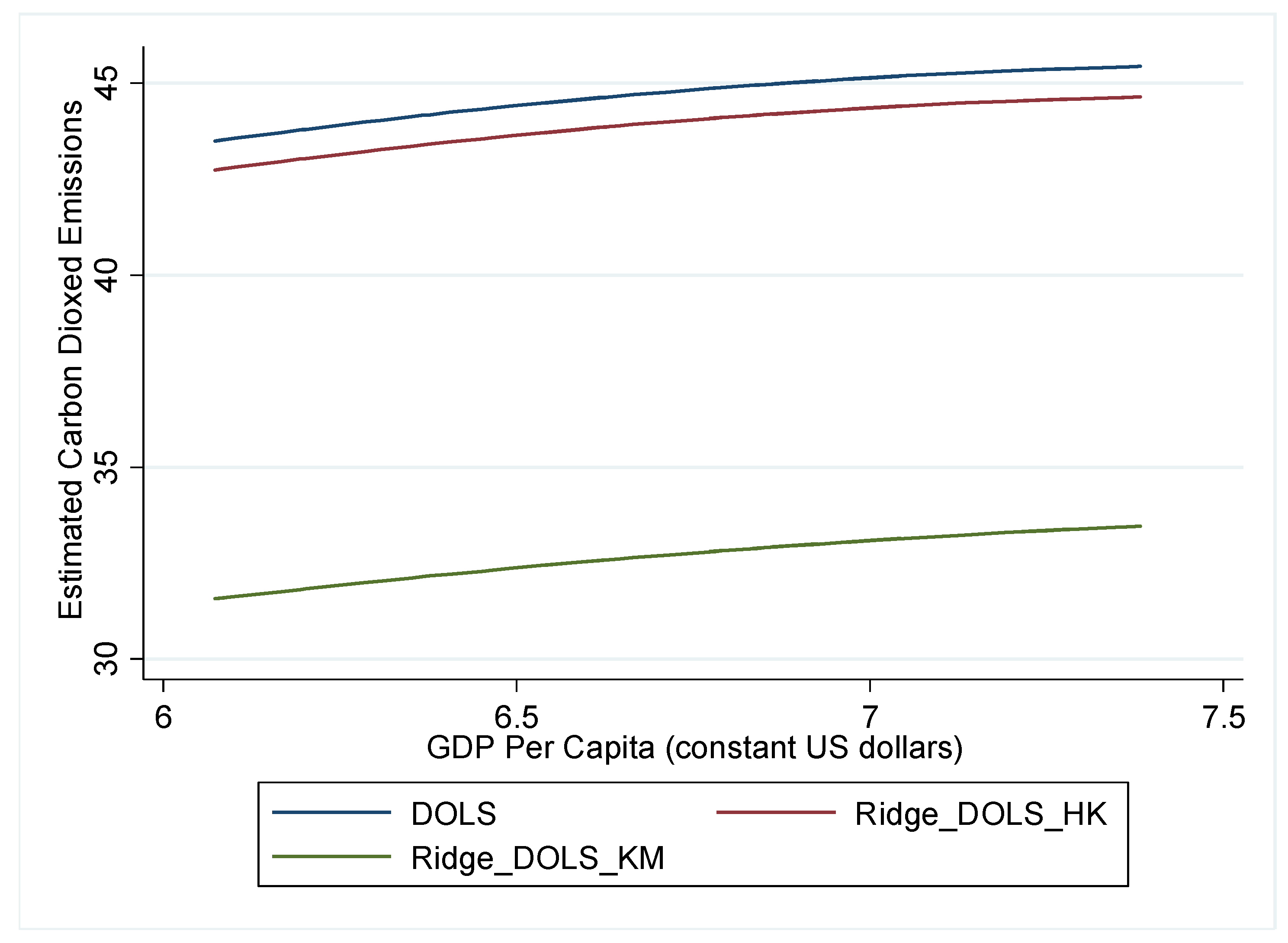
4.1. Environmental Kuznets Curve

4.1.1. Model and Data

In this section, we illustrate the benefit of the new method by applying it on the EKC for Turkey. A recent paper by Akbostanci et al. [27] found evidence of the EKC in Turkey. The EKC may be expressed as follows:

$$\ln \left(C{O}_{2t}\right)=\alpha +{\beta }_1\ln \left(Y_t\right)+{\beta }_2\ln {\left(Y_t\right)}^2+{\epsilon }_t,$$

(11)

where $C{O}_{2t}$ is the carbon dioxide emission per capita and $Y_t$ is the gross domestic product (GDP) per capita in constant U.S. dollars (baseyear 2000) as the economic indicator. The data is on a yearly frequency and covers the time period from 1960–2013. The data is displayed in Figure 1, and deceptive statistics of the growth rates are found in

Table 2. Descriptive statistics. GDP: gross domestic product.

Variable	Mean	Standard Deviation	Kurtosis	Skewness
GDP Growth rate	2.64	3.95	3.11	−0.76
Carbon Dioxide emission growth rate	3.67	5.48	3.91	−0.19
Energy consumption growth rate	2.60	4.00	3.44	−0.69

(in growth rates, since the time series is integrated of order one). Moreover, all variables are upward trending, which is expected for a country where the economy still has some challenges before being fully developed. Furthermore, there are no clear structural breaks. We may possibly find a potential stochastic trend around a deterministic trend. In Table 2, where descriptive statistics are presented, we can see that the average growth rate is around 3% for all variables. Furthermore, there are some signs of negative skewness and a positive kurtosis. Thus, some minor deviations from a normal distribution can be found. In Equation (11), we should, in accordance to the EKC, expect that ${\beta }_1>0$ and ${\beta }_2<0$. This implies that the EKC proposes that economic progress initially leads to environmental deterioration, but that after a certain level of economic development, a society starts to improve its environmental responsibility and there is a reduction in the level of environmental degradation. Essentially, this implies that economic growth is good for the environment in the long-run. Thus, initial economic growth will lead to environmental degradation but eventually, as the income level increases, the increase will sequentially diminish, and at a certain income level, environmental degradation will decrease, and as prosperity grows this will sequentially lead to a less polluting environment. Consequently, when transitioning towards a more industrialized country, we see in the data that the emission of carbon dioxide will increase, but after reaching a certain income level we will in fact reduce environmental degradation. This inverted U-shaped relationship between income and emission data is usually considered to be caused by a willingness of individuals with a higher income to spend more money on improving the environment. The issues when estimating Equation (11) are firstly that the variables are non-stationary, which will be shown using the augmented Dickey Fuller (ADF) test, as well as the generalized least square (ADF-GLS) version of the augmented Dickey-Fuller test. Secondly, it is clear that reversed causality may exist. The third problem is the apparent multicollinearity issue between $\ln (Y_t)$ and $\ln {(Y_t)}^2$. The first problem is easily avoided by demonstrating that the variables, in fact, are cointegrated by means of Johansen’s cointegration test. The second problem may be solved using the DOLS estimator suggested by Stock and Watson [1]. The third problem may be solved using the new Ridge DOLS estimator suggested in this paper. An advantage of our new approach is that to estimate our suggested Ridge DOLS estimator, one can simply apply the R package glmnet, and include leads and lags of the independent variables as regressors (R is a free open source statistical software).

4.1.2. Result Discussion

Table 3. Unit root tests.

ADF Test
	Levels	First differences	5% Critical values
$\ln \left(C{O}_{2t}\right)$	−2.780	−4.947	−3.498
$\ln \left(Y_t\right)$	−3.222	−5.001	−3.498
$\ln {\left(Y_t\right)}^2$	−3.534	−5.672	−3.498
GLS-ADF Test
	Levels	First differences	5% Critical values
$\ln \left(C{O}_{2t}\right)$	−0.787	−4.750	−3.171
$\ln \left(Y_t\right)$	−2.935	−4.768	−3.171
$\ln {\left(Y_t\right)}^2$	−2.976	−4.886	−3.171

Note: $C{O}_{2t}$ is the carbon dioxide emission per capita and $Y_t$ is the GDP per capita in constant U.S. dollars.

shows the results from the ADF test and the GLS version of the augmented Dickey-Fuller test with a deterministic trend where the Schwartz information criteria is used to decide the lag length. For the ADF test, the two original variables are clearly non-stationary, while the square of the carbon dioxide emission level is stationary at a 5% level of significance. However, when looking at the more powerful GLS version of the ADF test, all variables are non-stationary at a 5% significance level. The significant coefficient for the square of the carbon dioxide (when using the ADF test) is most likely due to a type I error. The reason is that the variable is non-stationary for both tests; there is no reason to believe that a square transformation makes a variable stationary. Therefore, we may proceed and test for cointegration. We apply Johansen’s cointegration test, where the Schwartz information criterion is used to determine the lag length, and the result is found in

Table 4. Johansen’s cointegration test.

	Trace Test		Maximum Eigenvalue Test
No. of cointegration vectors	Statistic	5% Critical Values	Statistic	5% Critical Values
None *	29.92	29.80	20.46	21.13
At most 1	11.46	15.49	10.87	14.26
At most 2	0.59	3.84	0.59	3.84

. The trace statistic identifies a significant cointegration relation at a 5% level of significance, while based on the maximum eigenvalues there is a significant relationship only at a 10% level of significance. In conclusion, this result indicates that a long-run cointegrating relationship exists between per capita carbon dioxide emission and the per capita GDP. Therefore, the prerequisites are satisfied, and we proceed and estimate Equation (11) using the DOLS and the Ridge regression version of the DOLS estimator. The result from the DOLS and the Ridge regression version of the DOLS estimator is found in

Table 5. DOLS and Ridge DOLS.

	DOLS			Ridge DOLS Using ${\widehat{\mathit{k}}}_{\mathit{H}\mathit{K}}$			Ridge DOLS Using ${\widehat{\mathit{k}}}_{\mathit{G}\mathit{M}}$
Variables	Coef.	S.E.	t-stat	Coef.	S.E.	t-stat	Coef.	S.E.	t-stat
$\ln (Y_t)$	11.83	0.89	13.37	11.63	0.84	13.93	8.29	0.52	16.04
$\ln {(Y_t)}^2$	−0.77	0.06	−11.86	−0.76	0.06	−12.22	−0.51	0.04	−13.04

Note: The standard error or the Ridge DOLS estimator are bootstrapped using residual based bootstrapping. DOLS is the dynamic OLS estimator. ${\widehat{k}}_{HK}$ and ${\widehat{k}}_{GM}$ are the ridge estimators suggested in Hoerl and Kennard [9,10] and Kibria [11] respectively. $Y_t$ is the GDP per capita in constant U.S. dollars.

. Based on the result in Table 5, it is clear that the length of the vector decreases when using the Ridge DOLS estimator. The standard error decreases when using the Ridge DOLS, and it is minimized when applying the ${\widehat{k}}_{GM}$ estimator of k. The t-statistics also increases when using the Ridge DOLS instead of the ordinary DOLS. Thus, a substantial amount of precision is gained when using Ridge DOLS instead of the ordinary DOLS. In Figure 2, the different long-term Kuznets curves using different estimators are found. Here, one can see that the effect of increasing the GDP per capita decreases when applying the Ridge DOLS estimator. Hence, by applying DOLS in the presence of multicollinearity, there is a considerable risk of overestimating the Kuznets curve. Therefore, this demonstration highlights the importance of taking this into account when estimating this the EKC, but this generic problem is also of high relevance for other types of problems in the field of energy economics.

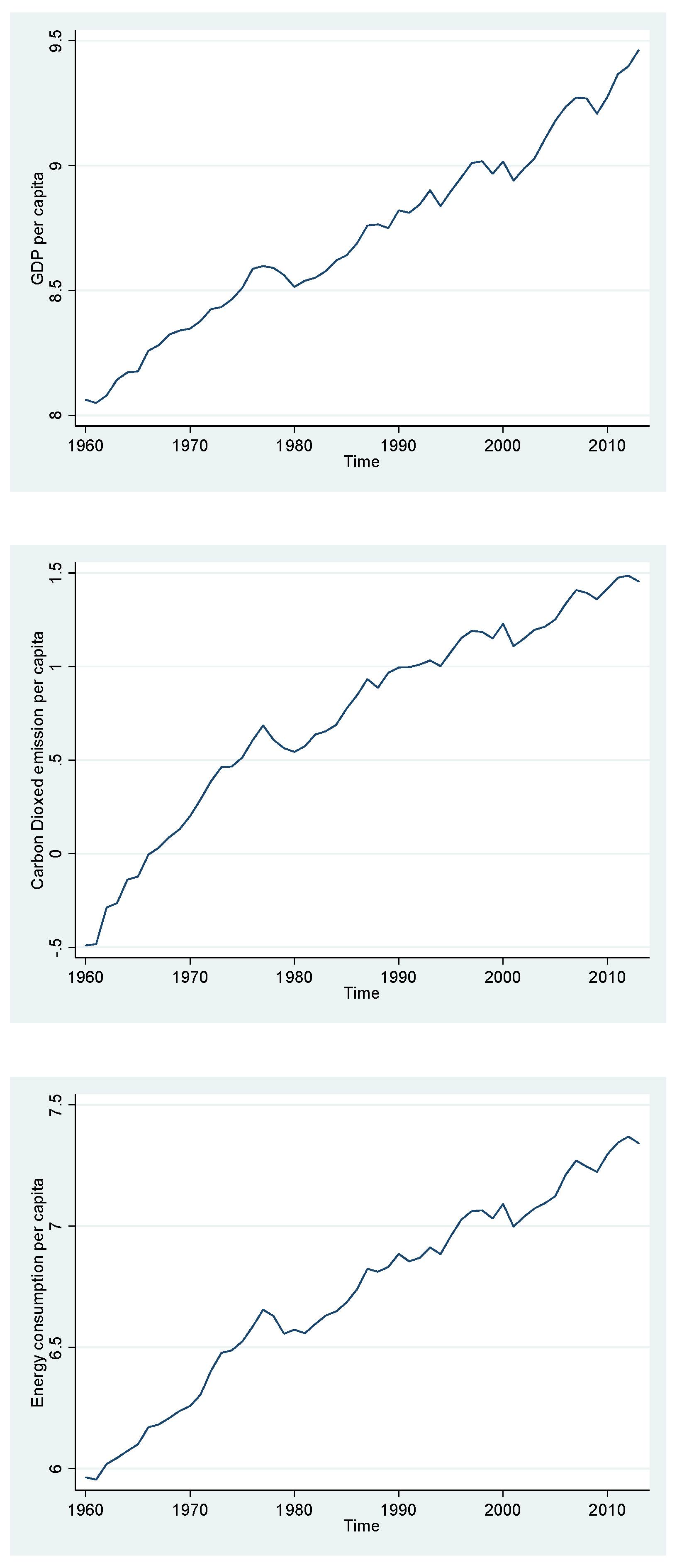
4.2. CO₂ Emissions, Energy Consumption and Economic Growth Nexus

4.2.1. Model and Data

Another related, important model in this field of research is the effect of energy consumption and economic growth on CO₂ emissions. For instance, in studies by Aspergis [23] and Belke et al. 3, DOLS is employed to estimate the following model:

$$\ln \left(C{O}_{2t}\right)=\alpha +{\beta }_1\ln \left(Y_t\right)+{\beta }_2\ln {\left(Y_t\right)}^2+{\beta }_2\ln \left(E_t\right)+{\epsilon }_t,$$

(12)

where $E_t$ is the energy consumption per capita, while the other variables are defined in Equation (11). Thus, this is merely an extended version of the Kuznets curve where energy consumption is added. Energy consumption is added in the above-mentioned paper since it has a considerable impact on environmental degradation. A focus on reducing per capita energy consumption is considered to be an effective method for decreasing carbon dioxide emissions; therefore. e.g., Asperigis (2016) argues that the variable should be included when estimating the EKC. The data covers the time period from 1960–2013. The procedure is identical to that of the Kuznets curve, where we used a unit root test and a cointegration test to establish that a linear combination of the variables is stationary, and then the DOLS and the new Ridge DOLS estimator to estimate the coefficients of Equation (12).

4.2.2. Result Discussion

From

Table 6. Unit root tests.

ADF Test
	Levels	First differences	5% Critical values
$\ln \left(C{O}_{2t}\right)$	−2.780	−4.947	−3.498
$\ln \left(Y_t\right)$	−3.222	−5.001	−3.498
$\ln {\left(Y_t\right)}^2$	−3.534	−5.672	−3.498
$\ln \left(E_t\right)$	−2.786	−5.522	−3.498
GLS-ADF Test
	Levels	First differences	5% Critical values
$\ln \left(C{O}_{2t}\right)$	−0.787	−4.750	−3.171
$\ln \left(Y_t\right)$	−2.935	−4.768	−3.171
$\ln {\left(Y_t\right)}^2$	−2.976	−4.886	−3.171
$\ln \left(E_t\right)$	−4.789	−2.035	−3.171

Note: $C{O}_{2t}$ is the carbon dioxide emission per capita and $Y_t$ is the GDP per capita in constant U.S. dollars.

and

Table 7. Johansen cointegration tests.

	Trace Test		Maximum Eigenvalue Test
No. of cointegration vectors	Statistic	5% Critical Values	Statistic	5% Critical Values
None	50.28	47.86	26.87	27.58
At most 1	23.41	29.80	19.07	21.13
At most 2	4.34	15.49	3.90	14.26
At most 3	0.44	3.84	0.44	3.84

we see that energy consumption also contains a unit root, and that a cointegrating vector exists using the same techniques as in the previous example using the EKC curve. Once again, we may see, using the trace statistic, that a significant cointegration relation at a 5% level of significance exists, and for the maximum eigenvalue that there is only a significant relationship at a 10% level of significance. This confirms that a long-term relationship exists between the variables, and that the assumptions for estimating a DOLS model are satisfied. Therefore, we proceed and estimate Equation (12) using the DOLS and the Ridge DOLS estimator. The correlation matrices in levels and first differences are shown in

Table 8. Correlation matrix of explanatory variables in levels.

	$\ln \left(Y_t\right)$	$\ln {\left(Y_t\right)}^2$	$\ln {\left(Y_t\right)}^2$
$\ln \left(Y_t\right)$	1	-	-
$\ln {\left(Y_t\right)}^2$	0.99	1	-
$\ln \left(E_t\right)$	0.99	0.99	1

Note: $Y_t$ is the GDP per capita in constant U.S. dollars and $E_t$ is the energy consumption per capita.

and

Table 9. Correlation matrix of explanatory variables in first differences.

	$\ln \left(Y_t\right)$	$\ln {\left(Y_t\right)}^2$	$\ln {\left(Y_t\right)}^2$
$\ln \left(Y_t\right)$	1	-	-
$\ln {\left(Y_t\right)}^2$	0.99	1	-
$\ln \left(E_t\right)$	0.73	0.71	1

Note: $Y_t$ is the GDP per capita in constant U.S. dollars and $E_t$ is the energy consumption per capita.

respectively. From these tables, it is clear, that there are very high correlations in levels (which may be due to spurious correlations). Therefore, we also analyze the data in first differences (which may be an estimate of the residual series which we use in the design of the experiment to induce correlation); then a rather high correlation remains between the variables (from 0.71 up to 0.99). The result from the standard DOLS and the Ridge DOLS estimators are found in

Table 10. DOLS and Ridge DOLS.

	DOLS			Ridge DOLS Using ${\widehat{\mathit{k}}}_{\mathit{H}\mathit{K}}$			Ridge DOLS Using ${\widehat{\mathit{k}}}_{\mathit{G}\mathit{M}}$
Variables	Coef.	S.E.	t-stat	Coef.	S.E.	t-stat	Coef.	S.E.	t-stat
$\ln (Y_t)$	6.46	0.76	8.54	5.77	0.60	9.66	4.96	0.49	10.03
$\ln {(Y_t)}^2$	−0.46	0.05	−9.64	−0.41	0.04	−9.96	−0.36	0.03	−10.80
$\ln (E_t)$	1.06	0.12	8.61	1.08	0.11	9.50	1.17	0.11	10.73

Note: The standard error or the Ridge DOLS estimator are bootstrapped using residual based bootstrapping. DOLS is the dynamic OLS estimator. ${\widehat{k}}_{HK}$ and ${\widehat{k}}_{GM}$ are the ridge estimators suggested in Hoerl and Kennard [9,10] and Kibria [11] respectively. $Y_t$ is the GDP per capita in constant U.S. dollars and $E_t$ is the energy consumption per capita.

. The results are similar to those of the previous example, since the new Ridge DOLS method leads to a decrease in standard errors, and an increase of the t-statistics. We can also observe that the standard errors are minimized when using the Ridge DOLS with the ${\widehat{k}}_{GM}$ estimator of k. When controlling for energy consumption, the effect of income on the CO₂ emission decreases. This effect further decreases when applying the Ridge DOLS estimator, while for energy consumption, the value of the estimated coefficient increases.

5. Summary and Conclusions

A unique contribution of this paper consists of proposing ridge estimators (that we call Ridge DOLS) for the standard DOLS model. This novelty is empirically relevant, and directly useful in many applications within the research field of energy economics. Since a theoretical comparison is not possible, a simulation study has been conducted to compare the performance of the estimators. The simulation study demonstrates that the proposed shrinkage estimator (Ridge DOLS) outperforms the standard DOLS estimator in the presence of empirically relevant magnitudes of multicollinearity. In our simulations, it is especially evident that combining DOLS with the Ridge regression estimator suggested by Kibria [11] results in the best performance in terms of MSE. In order to demonstrate the empirical relevance, we applied our new approaches for the environmental Kuznets curve (EKC) for Turkey. For this data, evidence of a long-term relationship is found using the Johansen’s cointegration test. Thus, as is discussed in the introduction, our result is in line with previous research in this field. The conventional approach is to apply the DOLS method to measure the effect of income on carbon dioxide emissions. However, in this application it is illustrated that the new Ridge DOLS estimator has considerably lower MSE than the standard DOLS estimator. Moreover, in the presence of moderate magnitudes of multicollinearity, it is found that the standard DOLS overestimates the effect of income on carbon dioxide emission. Therefore, when considering all the circumstances of this empirical situation, it is clear that the Ridge DOLS is superior to the standard DOLS. In our second empirical example, we augment the EKC curve by adding energy consumption. The result is similar to our previous example, and Ridge DOLS exhibit smaller standard errors than the traditional DOLS method. In conclusion, this paper clearly illustrates that the new Ridge DOLS method increases the precision when estimating parameters of cointegrated regression models in the presence of multicollinearity. Since correlation among the variables in the cointegration vector is empirically a very common phenomenon (which, for instance, is illustrated by our two examples), we argue that our new method is of substantial relevance for a wide variety of different situations in energy economics and environmental studies. As is illustrated in this paper, it is easily argued that the use of an adequate estimator may, in many situations, have a direct effect on policy implications in this field of research.

References

1. Stock, J.H.; Watson, M. A simple estimator of cointegrating vectors in higher Order integrated systems. Econometrica 1993, 61, 783–820. [Google Scholar] [CrossRef]
2. Caballero, R.J. Small Sample Bias and Adjustment Costs. Rev. Econ. Stat. 1994, 76, 52–58. [Google Scholar] [CrossRef]
3. Belke, A.; Dobnik, F.; Dreger, C. Energy consumption and economic growth: New insights into the cointegration relationship. Energy Econ. 2011, 33, 782–789. [Google Scholar] [CrossRef]
4. Ouedraogo, N.S. Energy consumption and economic growth: Evidence from the economic community of West African States (ECOWAS). Energy Econ. 2013, 36, 637–647. [Google Scholar] [CrossRef]
5. Damette, O.; Seghir, M. Energy as a driver of growth in oil exporting countries? Energy Econ. 2013, 37, 193–199. [Google Scholar] [CrossRef] [Green Version]
6. Nasr, A.B.; Gupta, R.; Sato, J.R. Is there an environmental Kuznets curve for South Africa? A co-summability approach using a century of data. Energy Econ. 2015, 52, 136–141. [Google Scholar] [CrossRef]
7. Apergis, N.; Payne, J.E. CO2 emissions, energy usage, and output in Central America. Energy Policy 2009, 3, 3282–3286. [Google Scholar] [CrossRef]
8. Chen, S.; Chen, H. Oil prices and real exchange rates. Energy Econ. 2007, 29, 390–404. [Google Scholar] [CrossRef]
9. Hoerl, A.E.; Kennard, R.W. Ridge regression: Biased estimation for non-orthogonal problems. Technometrics 1970, 12, 55–67. [Google Scholar] [CrossRef]
10. Hoerl, A.E.; Kennard, R.W. Ridge Regression: Application to non-orthogonal problems. Technometrics 1970, 12, 69–82. [Google Scholar] [CrossRef]
11. Kibria, B.M.G. Performance of some new ridge regression estimators. Commun. Stat. Theory Methods 2003, 32, 419–435. [Google Scholar] [CrossRef]
12. Månsson, K.; Shukur, G. On ridge parameters in logistic regression. Commun. Stat. Theory Methods 2011, 40, 3366–3381. [Google Scholar] [CrossRef]
13. Stern, D.I. The rise and fall of the environmental Kuznets curve. World Dev. 2004, 32, 1419–1439. [Google Scholar] [CrossRef]
14. Al-Mulali, U.; Saboori, B.; Ozturk, I. Investigating the environmental Kuznets curve hypothesis in Vietnam. Energy Policy 2015, 76, 123–131. [Google Scholar] [CrossRef]
15. Ang, J.B. CO2 emissions, energy consumption, and output in France. Energy Policy 2007, 35, 4772–4778. [Google Scholar] [CrossRef]
16. Halicioglu, F. An econometric study of CO2 emissions, energy consumption, income and foreign trade in Turkey. Energy Policy 2009, 37, 1156–1164. [Google Scholar] [CrossRef] [Green Version]
17. Jalil, A.; Mahmud, S.F. Environment Kuznets curve for CO2 emissions: A cointegration analysis for China. Energy Policy 2009, 37, 5167–5172. [Google Scholar] [CrossRef] [Green Version]
18. Hamit-Haggar, M. Greenhouse gas emissions, energy consumption and economic growth: A panel cointegration analysis from Canadian industrial sector perspective. Energy Econ. 2012, 34, 358–364. [Google Scholar] [CrossRef]
19. Lean, H.H.; Smyth, R. CO2 emissions, electricity consumption and output in ASEAN. Appl. Energy 2010, 87, 1858–1864. [Google Scholar] [CrossRef]
20. Saboori, B.; Sulaiman, J. CO2 emissions, energy consumption and economic growth in Association of Southeast Asian Nations (ASEAN) countries: A cointegration approach. Energy 2013, 55, 813–822. [Google Scholar] [CrossRef]
21. Pao, H.; Tsai, C. CO2 emissions, energy consumption and economic growth in BRIC countries. Energy Policy 2010, 38, 7850–7860. [Google Scholar] [CrossRef]
22. Marrero, G. Greenhouse gases emissions, growth and the energy mix in Europe. Energy Econ. 2010, 32, 1356–1363. [Google Scholar] [CrossRef]
23. Aspergis, N. Environmental Kuznets curves: New evidence on both panel and country-level CO2 emissions. Energy Econ. 2016, 54, 263–271. [Google Scholar] [CrossRef]
24. Wang, S.S.; Zhou, D.Q.; Zhou, P.; Wang, Q.W. CO2 emissions, energy consumption and economic growth in China: a panel data analysis. Energy Policy 2011, 39, 4870–4875. [Google Scholar] [CrossRef]
25. Engle, R.F.; Granger, C.W.J. Co-Integration and Error Correction: Representation, Estimation, and Testing. Econometrica 1987, 55, 251–276. [Google Scholar] [CrossRef]
26. Gibbons, D.G. A simulation study of some ridge estimators. J. Am. Stat. Assoc. 1981, 76, 131–139. [Google Scholar] [CrossRef]
27. Akbostanci, E.; Türüt-Aşik, S.; Tunç, G.I. The relationship between income and environment in Turkey: Is there an environmental Kuznets curve? Energy Policy 2009, 37, 861–867. [Google Scholar] [CrossRef]
Figure 1. Time series plots of the data.
Sustainability 10 01315 g001
Figure 2. The EKC. Note: DOLS is the dynamic OLS estimator. Ridge_DOLS_HK is the Hoerl and Kennard [9,10] estimator and Ridge_DOLS_KM is the Kibria [11] estimator.
Sustainability 10 01315 g002