Towards Efficient Energy Management and Power Trading in a Residential Area via Integrating a Grid-Connected Microgrid


 , , and
Abstract
:1. Introduction
- Two heuristic approaches CSA and SA are implemented to schedule appliances for efficient power trading.
- An analysis is performed to investigate the fact that CSA and SA are adaptable and capable of making autonomous decisions for effective scheduling of an appliance and optimal power trading with a commercial grid.
- We enable a smart home to interact with the grid and make autonomous decisions for selling power to the grid for getting financial benefits.
- In order to validate the effectiveness of CSA and SA, extensive simulations are performed in MATLAB (2017a) and the performance parameters are total cost and PAR along with earnings.
- Simulation results show that our proposed scheme significantly reduces the electricity cost and PAR with earning maximization.
2. Related Work
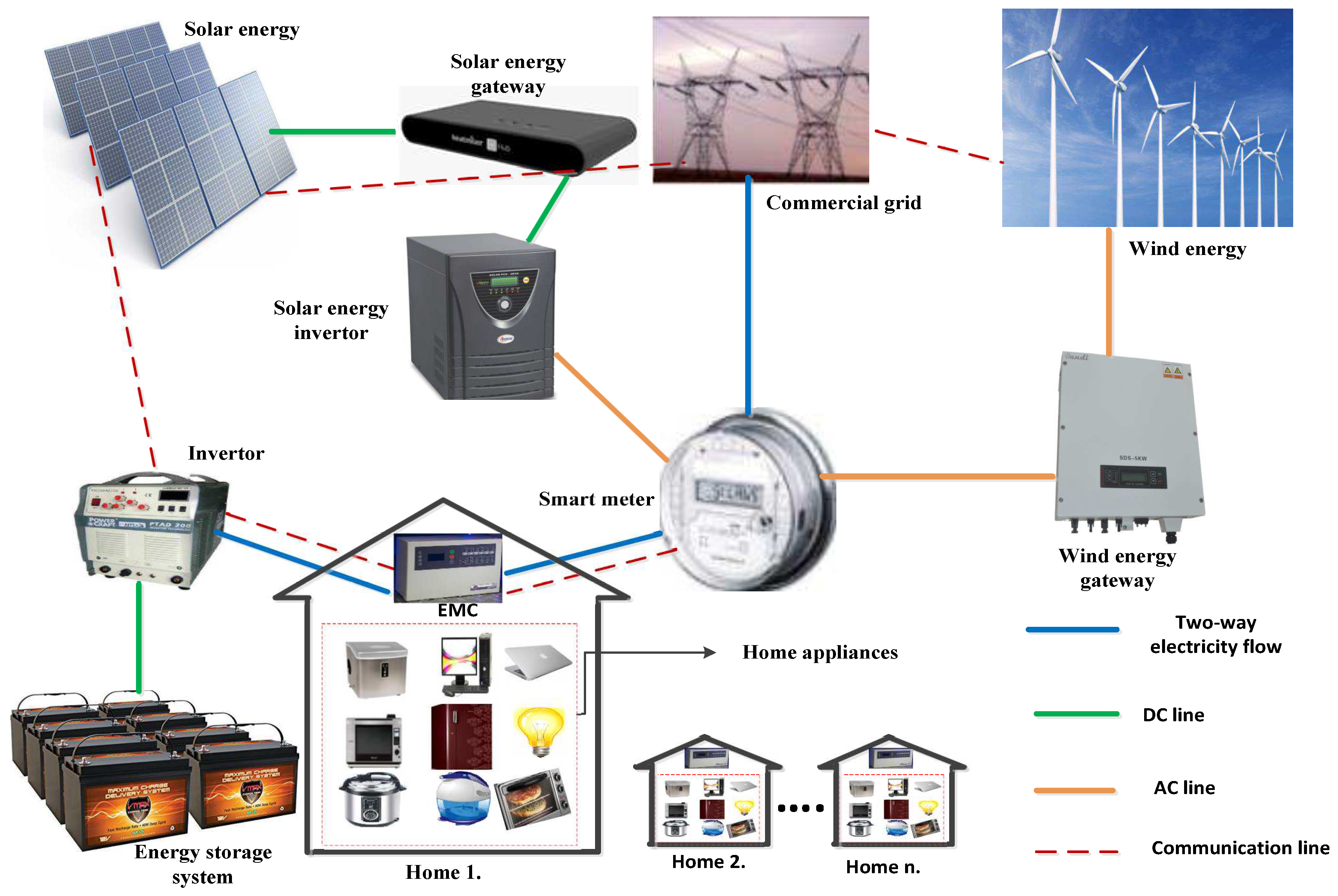
3. Proposed System Model
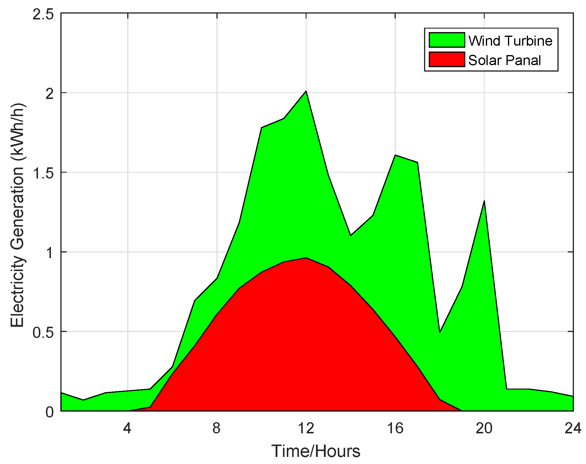
3.1. Microgrid
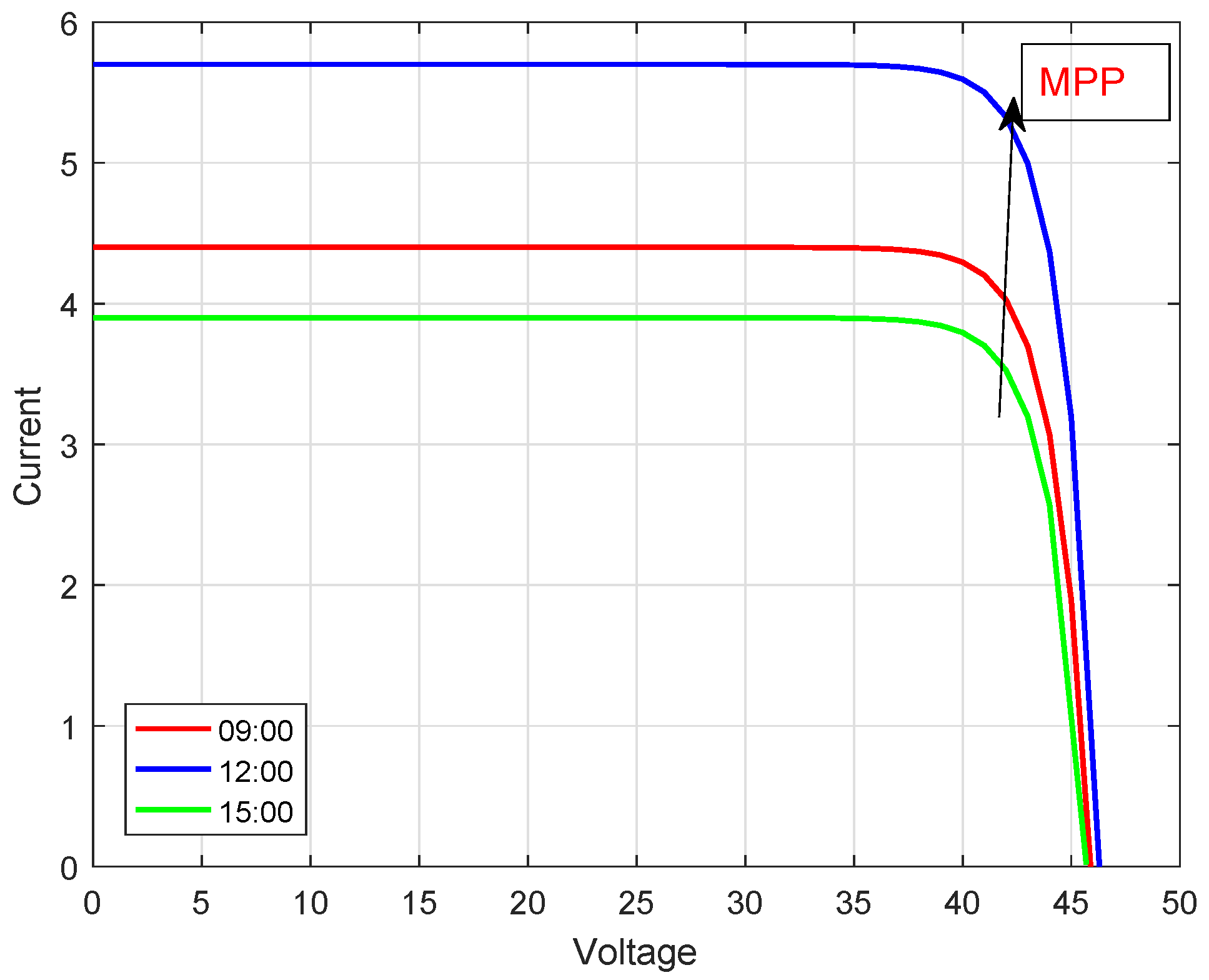
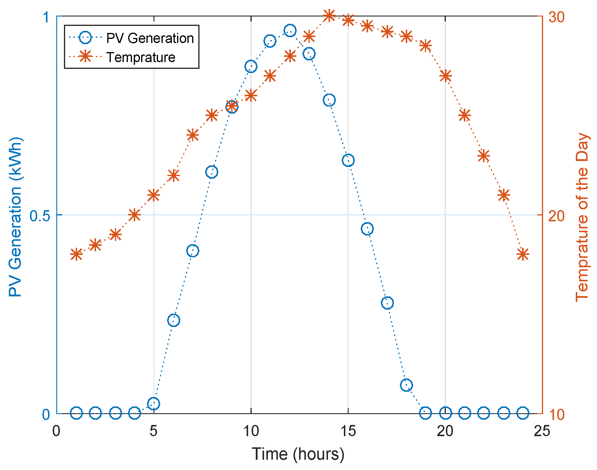
3.1.1. Solar Panel
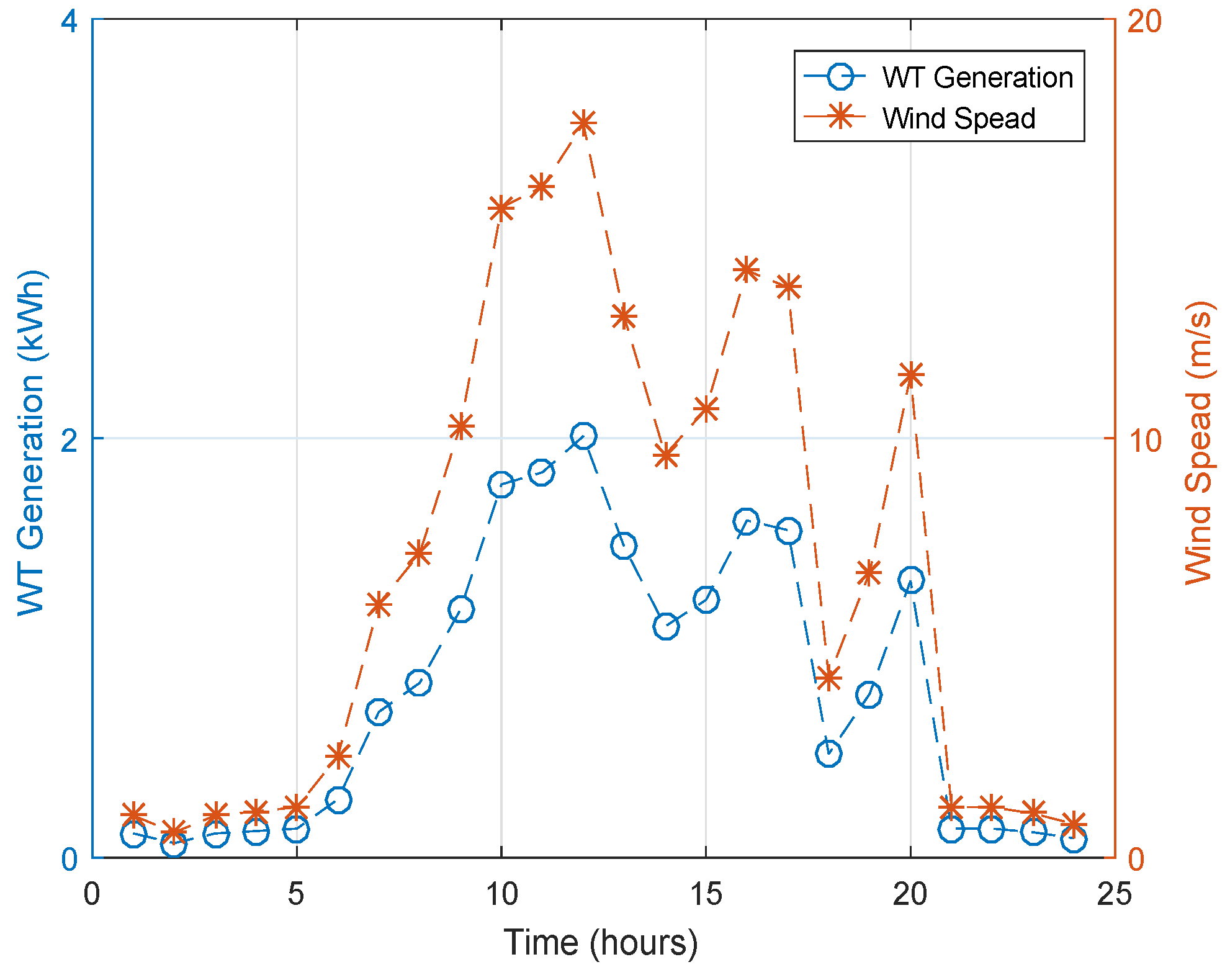
3.1.2. Wind Turbine
3.2. ESS
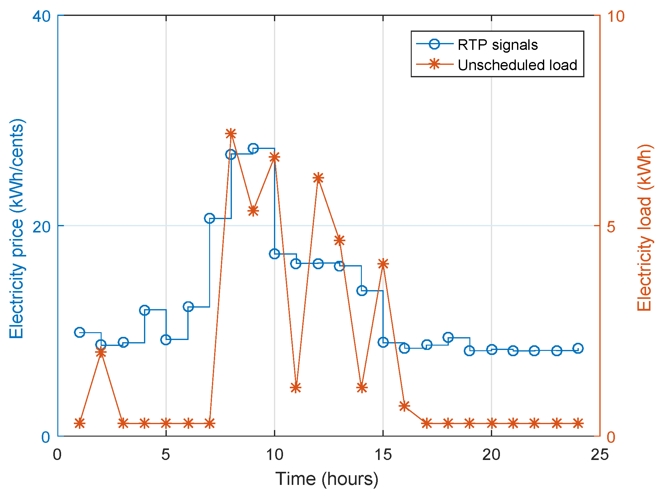
3.3. Household Electricity Load
3.4. Categorization of Load
3.4.1. Shiftable Appliances
3.4.2. Non-Interruptible Appliances
3.4.3. Base-Load Appliances
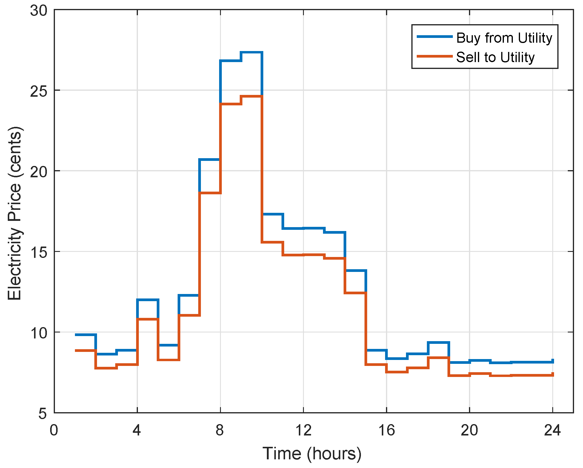
3.5. Electricity Tariff and Bill Calculation
4. Proposed Schemes
4.1. CSA
- Every cuckoo lays only one egg in the randomly chosen nest.
- Only the high-quality nests with the high quality eggs are considered for the next generation.
- Host nests are fixed and the host birds discover the eggs.
4.2. SA
5. Case Studies
6. Simulation Results
6.1. Case 1: Home without Energy Management and Microgrid
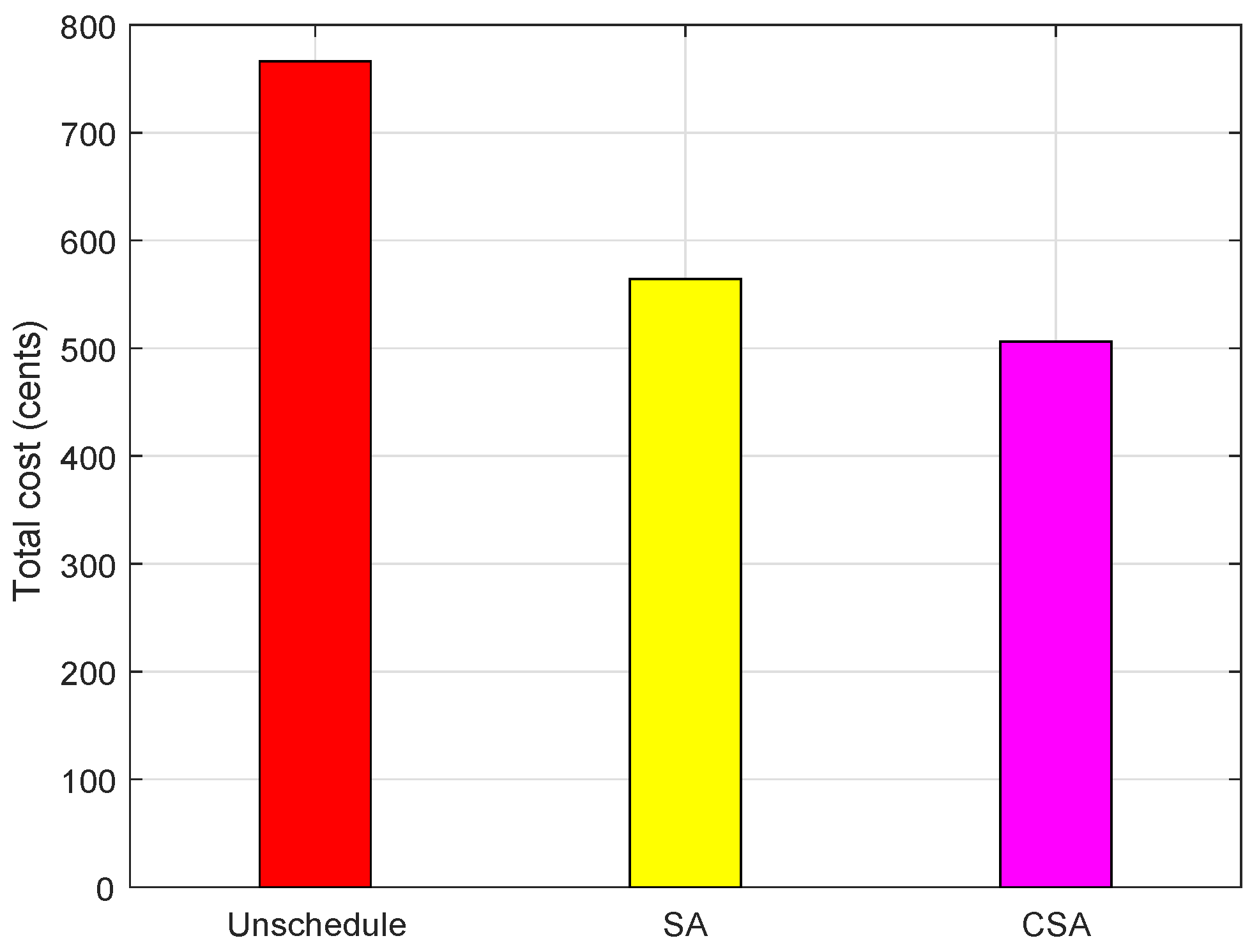
6.2. Case 2: Home with Energy Management but without Microgrid
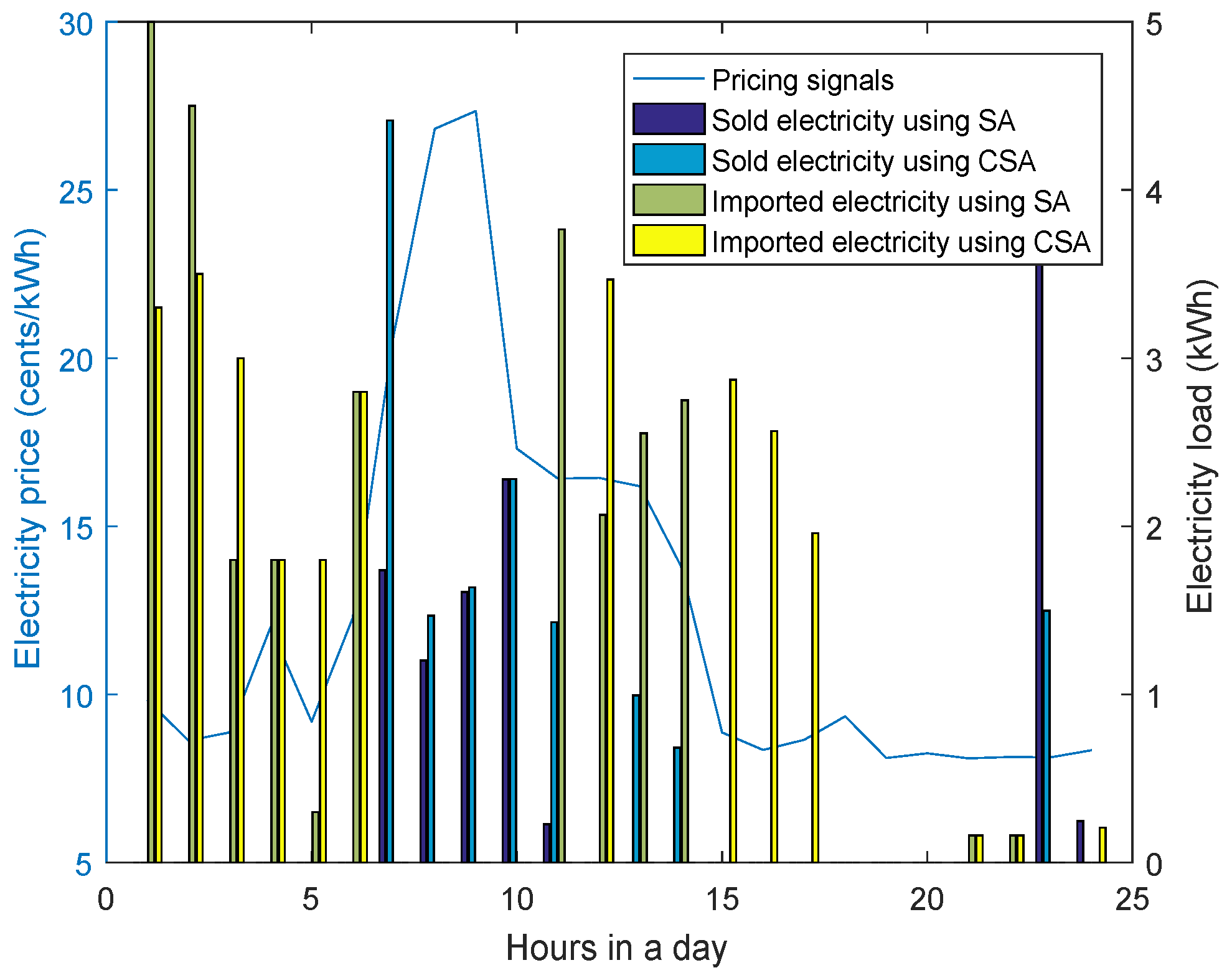
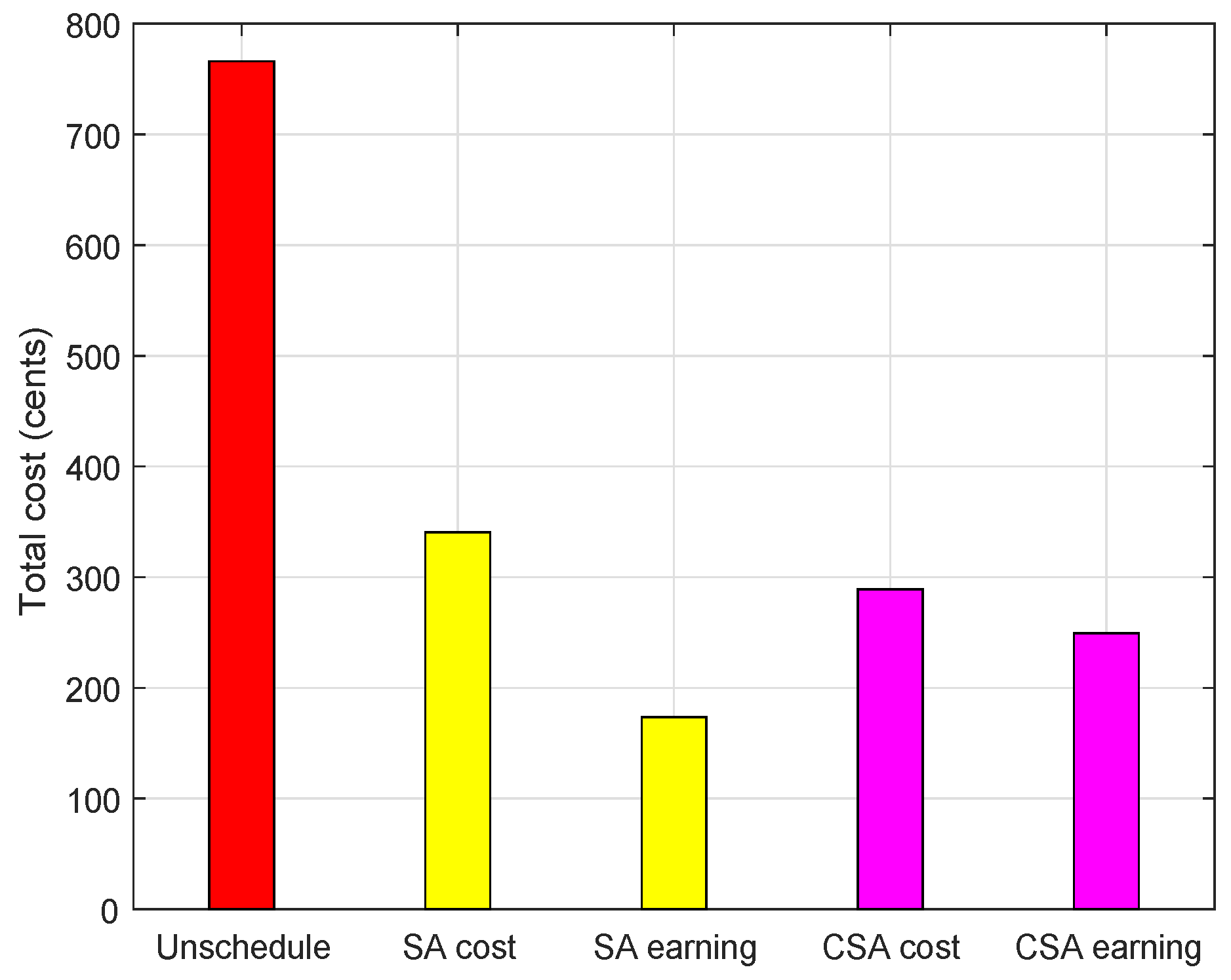
6.3. Case 3: Home with Energy Management and Microgrid
6.4. Performance Comparison
7. Conclusions
Acknowledgments
Author Contributions
Conflicts of Interest
Nomenclature
| t | Single time interval |
| T | Shows complete time intervals/day |
| Set of all appliances | |
| Set of shiftable appliances | |
| Non-interruptible appliances | |
| Set of appliances belonging to the base-load category | |
| Single appliance from shiftable category | |
| Single appliance from non-interruptible category | |
| Single appliance from base-load category | |
| Hourly power consumption of shiftable appliances | |
| Hourly power consumption of non-interruptible appliances | |
| Hourly power consumption of base-load appliances | |
| Shows electricity demand of shiftable appliances in a home | |
| Shows electricity demand of non-interruptible appliances in a home | |
| Shows electricity demand of base-load appliances in a home | |
| Show ON/OFF state of shiftable appliances category | |
| Show ON/OFF state in non-interruptible category | |
| Show ON/OFF state in base-load category | |
| Hourly electricity consumption tariff | |
| Per day electricity cost shiftable appliances | |
| Per day electricity cost against non-interruptible appliances | |
| Per day electricity cost against base load appliances | |
| Hourly cost against shiftable appliances | |
| Hourly cost against non-interruptible appliances | |
| Hourly cost against base load appliances | |
| Hourly electricity cost against all category of appliances | |
| Total hourly cost | |
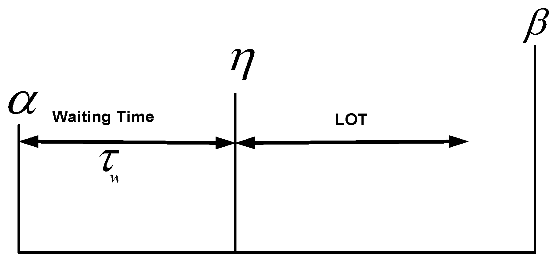
| Show possible earliest starting time of each appliance | |
| Show possible least ending time of each appliance | |
| Show possible starting execution of each appliance | |
| Demonstrates waiting time | |
| kv | Kilovolt |
| Kilowatt | |
| h | Hour |
| M | Microgrid |
| E | Energy generated from microgrid |
| m | Each source in microgrid |
| p | Power generation from solar panel |
| Power generation from wind turbine | |
| Stored electricity in ESS | |
| Charging of ESS | |
| Discharging of ESS | |
| ESS efficiency | |
| The capacity of wind turbine | |
| The capacity of solar panel | |
| The capacity of ESS | |
| Electricity purchasing rate | |
| Electricity selling rate | |
| Hourly cost against imported electricity | |
| Total cost against imported electricity for a day | |
| Hourly sold electricity | |
| Total sold electricity | |
| Hourly earnings | |
| Total per day earnings |
References
- Benzi, F.; Anglani, N.; Bassi, E.; Frosini, L. Electricity smart meters interfacing the households. IEEE Trans. Ind. Electron. 2011, 58, 4487–4494. [Google Scholar] [CrossRef]
- Evangelisti, S.; Lettieri, P.; Clift, R.; Borello, D. Distributed generation by energy from waste technology: A life cycle perspective. Process Saf. Environ. Prot. 2015, 93, 161–172. [Google Scholar] [CrossRef]
- Tascikaraoglu, A.; Boynuegri, A.R.; Uzunoglu, M. A demand side management strategy based on forecasting of residential renewable sources: A smart home system in Turkey. Energy Build. 2014, 80, 309–320. [Google Scholar] [CrossRef]
- Demand Side Response in the Domestic Sector—A Literature Review of Major Trial; Department of Energy and Climate Change: London, UK, 2012.
- Khalid, A.; Javaid, N.; Guizani, M.; Alhussein, M.; Aurangzeb, K.; Ilahi, M. Towards dynamic coordination among home appliances using multi-objective energy optimization for demand side management in smart buildings. IEEE Access 2018. [Google Scholar] [CrossRef]
- Albadi, M.H.; El-Saadany, E.F. A summary of demand response in electricity markets. Electr. Power Syst. Res. 2008, 78, 1989–1996. [Google Scholar] [CrossRef]
- Avci, M.; Erkoc, M.; Rahmani, A.; Asfour, S. Model predictive HVAC load control in buildings using real-time electricity pricing. Energy Build. 2013, 60, 199–209. [Google Scholar] [CrossRef]
- Yang, J.; Zhang, G.; Ma, K. Matching supply with demand: A power control and real time pricing approach. Int. J. Electr. Power Energy Syst. 2014, 61, 111–117. [Google Scholar] [CrossRef]
- Ahmad, A.; Khan, A.; Javaid, N.; Hussain, H.M.; Abdul, W.; Almogren, A.; Alamri, A.; Azim Niaz, I. An optimized home energy management system with integrated renewable energy and storage resources. Energies 2017, 10, 549. [Google Scholar] [CrossRef]
- Aslam, S.; Iqbal, Z.; Javaid, N.; Khan, Z.A.; Aurangzeb, K.; Haider, S.I. Towards Efficient Energy Management of Smart Buildings Exploiting Heuristic Optimization with Real Time and Critical Peak Pricing Schemes. Energies 2017, 10, 2065. [Google Scholar] [CrossRef]
- Van der Stelt, S.; AlSkaif, T.; van Sark, W. Techno-economic analysis of household and community energy storage for residential prosumers with smart appliances. Appl. Energy 2018, 209, 266–276. [Google Scholar] [CrossRef]
- Liu, R.S.; Hsu, Y.F. A scalable and robust approach to demand side management for smart grids with uncertain renewable power generation and bi-directional energy trading. Int. J. Electr. Power Energy Syst. 2018, 97, 396–407. [Google Scholar] [CrossRef]
- Bradac, Z.; Kaczmarczyk, V.; Fiedler, P. Optimal scheduling of domestic appliances via milp. Energies 2014, 8, 217–232. [Google Scholar] [CrossRef]
- Zhu, Z.; Tang, J.; Lambotharan, S.; Chin, W.H.; Fan, Z. An integer linear programming based optimization for home demand-side management in smart grid. In Proceedings of the 2012 IEEE PES Innovative Smart Grid Technologies (ISGT), Washington, DC, USA, 16–20 January 2012; pp. 1–5. [Google Scholar]
- Zhang, D.; Evangelisti, S.; Lettieri, P.; Papageorgiou, L.G. Economic and environmental scheduling of smart homes with microgrid: DER operation and electrical tasks. Energy Convers. Manag. 2016, 110, 113–124. [Google Scholar] [CrossRef]
- Mohamed, F.A.; Koivo, H.N. Online management genetic algorithms of microgrid for residential application. Energy Convers. Manag. 2012, 64, 562–568. [Google Scholar] [CrossRef]
- Khan, M.A.; Javaid, N.; Mahmood, A.; Khan, Z.A.; Alrajeh, N. A generic demand-side management model for smart grid. Int. J. Energy Res. 2015, 39, 954–964. [Google Scholar] [CrossRef]
- Samadi, P.; Wong, V.W.; Schober, R. Load scheduling and power trading in systems with high penetration of renewable energy resources. IEEE Trans. Smart Grid 2016, 7, 1802–1812. [Google Scholar] [CrossRef]
- Qayyum, F.A.; Naeem, M.; Khwaja, A.S.; Anpalagan, A.; Guan, L.; Venkatesh, B. Appliance scheduling optimization in smart home networks. IEEE Access 2015, 3, 2176–2190. [Google Scholar] [CrossRef]
- Agnetis, A.; de Pascale, G.; Detti, P.; Vicino, A. Load scheduling for household energy consumption optimization. IEEE Trans. Smart Grid 2013, 4, 2364–2373. [Google Scholar] [CrossRef]
- Tushar, M.H.K.; Assi, C.; Maier, M.; Uddin, M.F. Smart microgrids: Optimal joint scheduling for electric vehicles and home appliances. IEEE Trans. Smart Grid 2014, 5, 239–250. [Google Scholar] [CrossRef]
- Erdinc, O. Economic impacts of small-scale own generating and storage units, and electric vehicles under different demand response strategies for smart households. Appl. Energy 2014, 126, 142–150. [Google Scholar] [CrossRef]
- Mary, G.A.; Rajarajeswari, R. Smart grid cost optimization using genetic algorithm. Int. J. Res. Eng. Technol. 2014, 3, 282–287. [Google Scholar]
- Javaid, N.; Ullah, I.; Akbar, M.; Iqbal, Z.; Khan, F.A.; Alrajeh, N.; Alabed, M.S. An intelligent load management system with renewable energy integration for smart homes. IEEE Access 2017, 5, 13587–13600. [Google Scholar] [CrossRef]
- Wang, Y.; Saad, W.; Han, Z.; Poor, H.V.; Başar, T. A game-theoretic approach to energy trading in the smart grid. IEEE Trans Smart Grid 2014, 5, 1439–1450. [Google Scholar] [CrossRef]
- Sheraz, A.; Syed, M.M.; Asif, K.; Sakeena, J.; Saad, S.K.; Nadeem, J. An efficient home energy management and power trading in smart grid. In Proceedings of the 12th International Conference on Innovative Mobile and Internet Services in Ubiquitous Computing (IMIS), Matsue, Japan, 4–6 July 2018. [Google Scholar]
- Song, Z.; Geng, X.; Kusiak, A.; Xu, C. Mining Markov chain transition matrix from wind speed time series data. Expert Syst. Appl. 2011, 38, 10229–10239. [Google Scholar] [CrossRef]
- Zubair, L. Diurnal and seasonal variation in surface wind at Sita Eliya, Sri Lanka. Theor. Appl. Climatol. 2002, 71, 119–127. [Google Scholar] [CrossRef]
- Shirazi, E.; Jadid, S. Optimal residential appliance scheduling under dynamic pricing scheme via HEMDAS. Energy Build. 2015, 93, 40–49. [Google Scholar] [CrossRef]
- Ding, Y.M.; Hong, S.H.; Li, X.H. A demand response energy management scheme for industrial facilities in smart grid. IEEE Trans. Ind. Inform. 2014, 10, 2257–2269. [Google Scholar] [CrossRef]
- Yang, X.S.; Deb, S. Cuckoo search via Lévy flights. In Proceedings of the World Congress on Nature & Biologically Inspired Computing, NaBIC 2009, Coimbatore, India, 9–11 December 2009; pp. 210–214. [Google Scholar]
- Merrikh-Bayat, F. A Numerical Optimization Algorithm Inspired by the Strawberry Plant. arXiv, 2014; arXiv:1407.7399. [Google Scholar]


| Appliances Category | Appliance Name | Power Rating (kW) | Earliest Starting Time (h) | Least Finishing Time (h) | LOT (h) |
|---|---|---|---|---|---|
| Shiftable appliances | Cooker hub | 3 | 6 | 10 | 1 |
| Cooker oven | 5 | 15 | 20 | 1 | |
| Microwave | 1.7 | 6 | 10 | 1 | |
| Laptop | 0.1 | 18 | 24 | 2 | |
| Desktop | 0.3 | 18 | 24 | 3 | |
| Vacuum cleaner | 1.2 | 9 | 17 | 1 | |
| Electrical car | 3.5 | 18 | 8 | 3 | |
| Non-interruptible appliances | Dish washer | 1.5 | 9 | 17 | 2 |
| Washing machine | 1.5 | 7 | 12 | 2 | |
| Spin dryer | 2.5 | 13 | 18 | 1 | |
| Base-load appliances | Interior lighting | 0.84 | 16 | 24 | 6 |
| Refrigerator | 0.3 | 1 | 24 | 24 |
| Parameters | Values |
|---|---|
| Host nests | 50 |
| Iterations | 2000 |
| Discovery-rate | 0.250 |
| n | 12 |
| Parameters | Values |
|---|---|
| Population size | 100 |
| Runners | 50 |
| Roots | 10 |
| Iterations | 2000 |
| n | 12 |
| Parameters | Values |
|---|---|
| 2 kW | |
| 1 kW | |
| 5 | |
| 25 | |
| 5 kW | |
| 90% | |
| 95% |
| Parameters | Case 1 | Case 2 | Case 3 | ||
|---|---|---|---|---|---|
| Technique | SA | CSA | SA | CSA | |
| Cost (cents) | 766 | 562.02 | 487.43 | 335.74 | 284.70 |
| PAR | 3.99 | 3.63 | 2.29 | 3.12 | 1.98 |
| Cost savings | 0 | 26.63% | 36.42% | 56.26% | 62.83% |
| Earnings (cents) | 0 | 0 | 0 | 173.39 | 249.39 |
© 2018 by the authors. Licensee MDPI, Basel, Switzerland. This article is an open access article distributed under the terms and conditions of the Creative Commons Attribution (CC BY) license (http://creativecommons.org/licenses/by/4.0/).
Share and Cite
Aslam, S.; Javaid, N.; Khan, F.A.; Alamri, A.; Almogren, A.; Abdul, W. Towards Efficient Energy Management and Power Trading in a Residential Area via Integrating a Grid-Connected Microgrid. Sustainability 2018, 10, 1245. https://doi.org/10.3390/su10041245
Aslam S, Javaid N, Khan FA, Alamri A, Almogren A, Abdul W. Towards Efficient Energy Management and Power Trading in a Residential Area via Integrating a Grid-Connected Microgrid. Sustainability. 2018; 10(4):1245. https://doi.org/10.3390/su10041245
Chicago/Turabian StyleAslam, Sheraz, Nadeem Javaid, Farman Ali Khan, Atif Alamri, Ahmad Almogren, and Wadood Abdul. 2018. "Towards Efficient Energy Management and Power Trading in a Residential Area via Integrating a Grid-Connected Microgrid" Sustainability 10, no. 4: 1245. https://doi.org/10.3390/su10041245
APA StyleAslam, S., Javaid, N., Khan, F. A., Alamri, A., Almogren, A., & Abdul, W. (2018). Towards Efficient Energy Management and Power Trading in a Residential Area via Integrating a Grid-Connected Microgrid. Sustainability, 10(4), 1245. https://doi.org/10.3390/su10041245