Article

Foodshed as an Example of Preliminary Research for Conducting Environmental Carrying Capacity Analysis

Department of Spatial Economy, Wrocław University of Environmental and Life Sciences, Grunwaldzka 55, 50-357 Wrocław, Lower Silesian, Poland
*
Author to whom correspondence should be addressed.
Sustainability 2018, 10(3), 882; https://doi.org/10.3390/su10030882
Submission received: 30 January 2018 / Revised: 8 March 2018 / Accepted: 16 March 2018 / Published: 20 March 2018

Abstract

:
Since the 1960s, we have had to face challenging problems in relation to uncontrolled urban development, the destruction of farmlands, and the need to protect natural resources. These challenges are still valid, particularly since dynamic increases in population, especially in cities, have created an increasing need for natural resources. Therefore, the spatial management of the city should take into account the actual use of resources by its inhabitants, as well as the availability of resources within a city and its surrounding suburban areas. Such surveys could be conducted in order to ensure that the basic needs and safety of the residents are met, i.e., in the context of food security. Thus, we recommend a tool that allows specifying the geographical area of food supply: the foodshed. We determined the foodshed based on the relationship between the places of food production and its consumption. Therefore, we delimitated the extent of foodshed area for the city of Wrocław, which reached ca. 56 km. Our work expanded the determination of foodshed boundaries by the delimitation of the city’s foodshed zones, and provided a more detailed analysis of the obtained product data. We obtained data about 98 places of food origin, 448 products, and 115 types of products. This analysis was conducted using Tableau Software (Seattle, WA, USA) and Dell Statistica Software (Round Rock, TX, USA), and the food zone was mapped using ArcGIS Software (Redlands, CA, USA). The main goal of the study was to present a framework for foodshed assessment that could be integrated into other analyses of a city’s sustainability in the context of environmental carrying capacity, and the development of the spatial management of a city in a more sustainable way. This preliminary analysis was carried out in order to emphasize the need for conducting an environmental carrying capacity analysis for the city.

1. Introduction

Since the 1960s, we have faced challenging problems relating to uncontrolled urban development, which has not recognized nor taken into account local conditions of non-economic environment ecosystem functions and their biophysical limits [1,2,3]. As a result, this uncontrolled development has had a significant impact on environmental quality [4,5]. The carrying capacity of the environment needs to be accurately estimated for cities, and included into urban planning and development [6,7] in order to meet urban residents’ needs in a sustainable way [8,9]. At present, there is no chance to develop sustainable cities when the basis of the ecological resources on which they depend is excluded from spatial policy [6]. This is especially urgent because urbanization is directly related to increasing demands for natural resources (soil and water), which provide the food and ecosystem services that are used by a city [10]. Therefore, there is a need to increase the number of human settlements and cities implementing, adopting, and integrating policies and plans that increase inclusiveness, the efficient use of natural resources, mitigation, and better adaptations to climate change [11]. These goals could be achieved by conducting an environmental carrying capacity analysis.
Environmental carrying capacity (ECC) is also known as the carrying capacity of the environment, carrying capacity, ecological capacity, and ecological resilience [12]. It is a concept and tool for the development of sustainable human settlements, especially in the face of the serious environmental degradation of air, water, and land [2]. According to Fogel (ed. 2005), ECC determines the threshold level of anthropopression at which decisions in the field of spatial planning can be considered consistent with principles of sustainable development [13]. Therefore, ECC is a powerful tool for spatial planning [14], as well as for environmental planning and management or strategic environmental assessment [12]. Wei et al. (2016) emphasized the necessity of conducting analyses of the environmental carrying capacity of metropolitan areas [15], especially now that more than half of the world’s population lives in cities [16,17,18], and the predicted population growth will be concentrated there [15,19,20]. As population growth occurs, resources become limited [21,22], and the boundaries of a city’s supply areas (territorial carrying capacity) are exceeded, which is connected with trade, import [23], and transportation improvement [24]. The ECC is most often verified by the use of environmental indicators such as ecological footprint (EF) and biocapacity (BC) [22,25,26,27,28,29,30,31]. The BC and EF enable the verification of whether the environmental productivity of a given area is able to satisfy rising human needs, or if the capacity of a given area has been overshot [26]. It provides challenging guidelines for the management of resources in more ecologically, socially and responsible ways [32]. As Sali et al. (2014) emphasized, “there is a need for conducting [an] analysis of city shape, its spatial limit and—connected with them—[the] amount of needed resources and area required to satisfy them” [24]. The main human need provided by the environment is food [32]. The analysis, which verifies the functioning of a city’s food system, is called foodshed [33,34].
Foodshed [33,34] is also known as production capacity, local food production capacity [35], or local foodshed carrying capacity [36]. It is defined as geographical area of food supply that verifies the interaction between urban consumption and peri-urban production, representing the food zone for urbanized areas [33,34]. The foodshed is defined briefly as a “local region [that] provides enough food products to feed its population” [37]. The calculation of foodshed can be conducted using two approaches, which enable discussions about the functioning of local food systems. The first approach, which was proposed by Hedden in 1929, is based on the relationship between places of food production and its consumer market [24,33]. This approach verifies the distribution flow of food [38], as well as the functioning of the entire food system, and its impact on the environment [33]. The second approach of local foodshed carrying capacity assessment enables the determination of the production capacity of potentially available land for peri-urban and intra-urban agriculture. This analysis is based on a number of factors, i.e., soil quality, the size of plots, access to irrigation water, and location [36]. Urban development projects have used the concept of the foodshed to emphasize that the production of local food ought to be a healthy, ecologically sustainable, and economically sustainable solution to issues surrounding development and lifestyle. The concept of the foodshed is especially pertinent now that recent food systems could be considered more global than local, which has a destructive impact on the environment and social communities. There has been an increase in the implementation of local food aspects into the sustainable strategies of urban growth plans [38], particularly as an element of the long-term security of urban food supply and municipal food policies, which could increase the sustainability of the city [39,40]. Although agriculture and the foodshed assessments appear in some metropolitan concepts, there is still a need to introduce the food analysis into the urban concept of sustainability. This need is especially strong because urban consumption centers are dependent on peri-urban and rural agricultural production areas [34], and urban agriculture is not enough to feed all of the inhabitants of the city [41]. Recently, there has been a revival of efforts to integrate urban agriculture and spatial planning [42]. Therefore, there is a need to implement an integrated spatial decision support system in an urban context [43] that takes into account all of the aspects of a city’s functioning (as food or other ecosystem services). Such an approach would enable the provision of spatial management in a more sustainable way that does not overshoot an urban area’s environmental capacity.
The main goal of this study was to present a framework for foodshed assessment that could be integrated with other analyses of a city’s sustainability in the context of environmental carrying capacity and the development of spatial management in a more sustainable way. In our research, we decided to conduct the analysis based on the first approach of foodshed determination, which verifies the interaction between food origin and its consumer market. Our work expands this approach through delimitating foodshed zones and providing a more detailed analysis of obtained product data. The following section introduces details regarding the study area, analysis database, and method of foodshed determination. In the third section, we describe the obtained results, which are discussed further in the fourth section. The final section presents our conclusions and suggestions for the possible use of method and statistical analyses and techniques (such as cluster analysis) in other contexts, such as accessibility to other ecosystem services in the city.

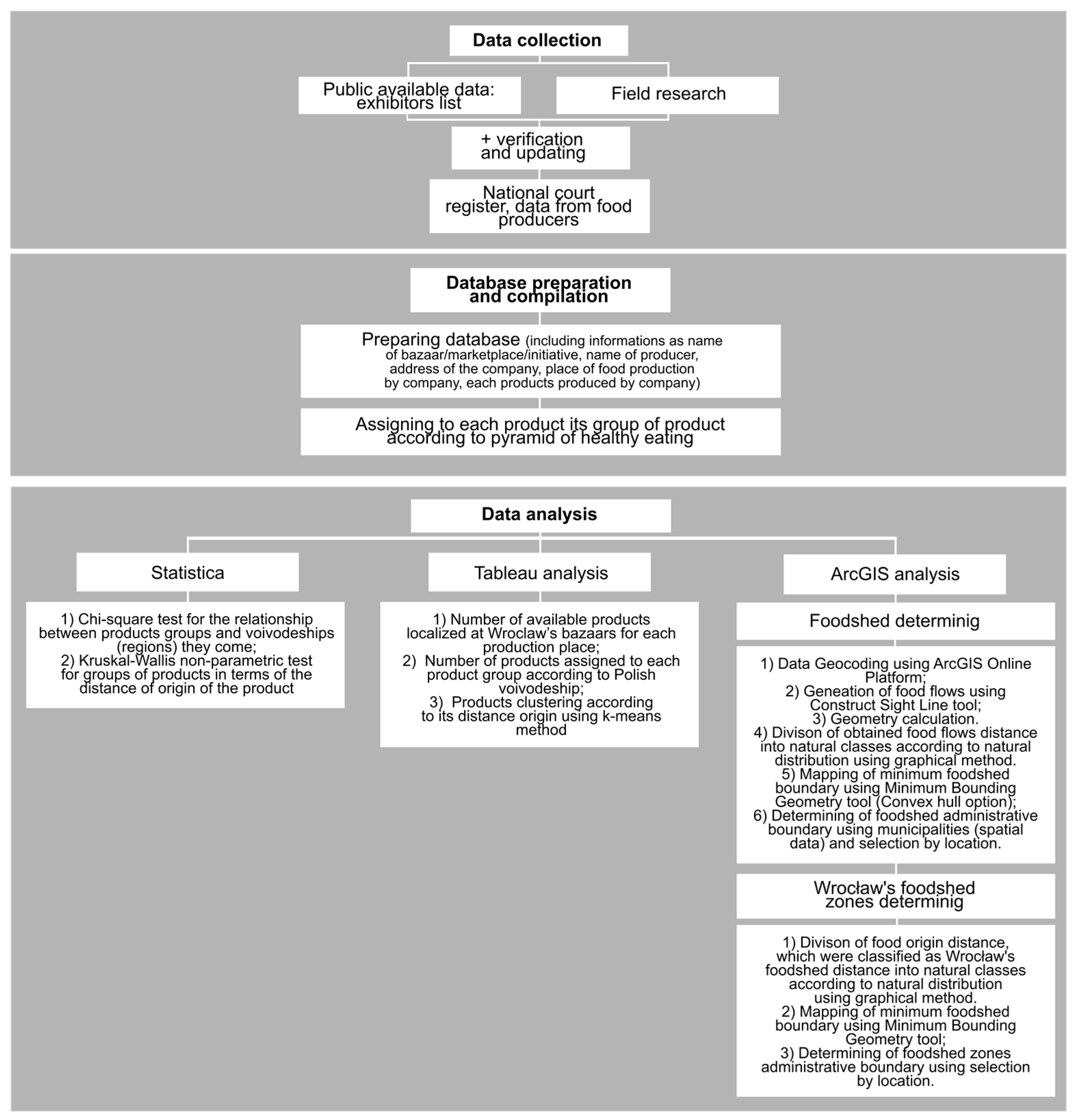
2. Materials and Methods

2.1. Study Area

Our analysis was conducted for the city of Wrocław, which is situated in southwestern Poland in central Europe. Wrocław is a metropolitan area with an area of 293 km2 and 637,000 inhabitants, which makes it the fourth biggest city in Poland (according to data of the Central Statistical Office of Poland as of 31 December 2016). Wrocław is known as a strongly transforming city with a highly spreading residential zone and suburban area [44]. Referring to the assumption that the foodshed determines the local food production capacity for a city and its surrounding area, we decided to extend obtained results regarding Wrocław’s foodshed boundary the suburban zone boundary, which consists of 10 municipalities with a total area of 1416.4 km2 [45]. Thus, the obtained foodshed area will be compared with a reference area (of Wrocław city and its suburban zone) of 1655.4 km2.
The research takes into account the largest urban markets, the most popular common bazaars, and also the bazaars and marketplaces offering products directly from farmers (Figure 1).
The largest urban markets that were included in the study are the TargPiast marketplace at Obornicka Street in the northern part of the city, and the Dolnośląskie Centrum Hurtu Rolno-Spożywczego S.A. (DCHRS) (Lower Silesian Center of Agricultural and Food Wholesale Market—LSCAFWM) at Giełdowa Street in the southern part of the city. The study also took into account the most popular common bazaars, such as the Targowisko na Świebodzkim (Bazaar at the Świebodzki Square)—located in a former railway station at Orląt Lwowskich Square—and the Hala Targowa (Market Square) at Piaskowa Street, which is located in the city centre. Furthermore, this research includes information obtained from bazaars and marketplaces that offer products directly from farmers, such as the Ekobazar at Tęczowa Street, the Bazaar Krótka Droga at Białoskórnicza Street (both of which are located in the city centre), and the Wrocławski Bazar Smakoszy (Wroclaw’s gourmets bazaar) at Hubska Street, which is located southeast of the city center.

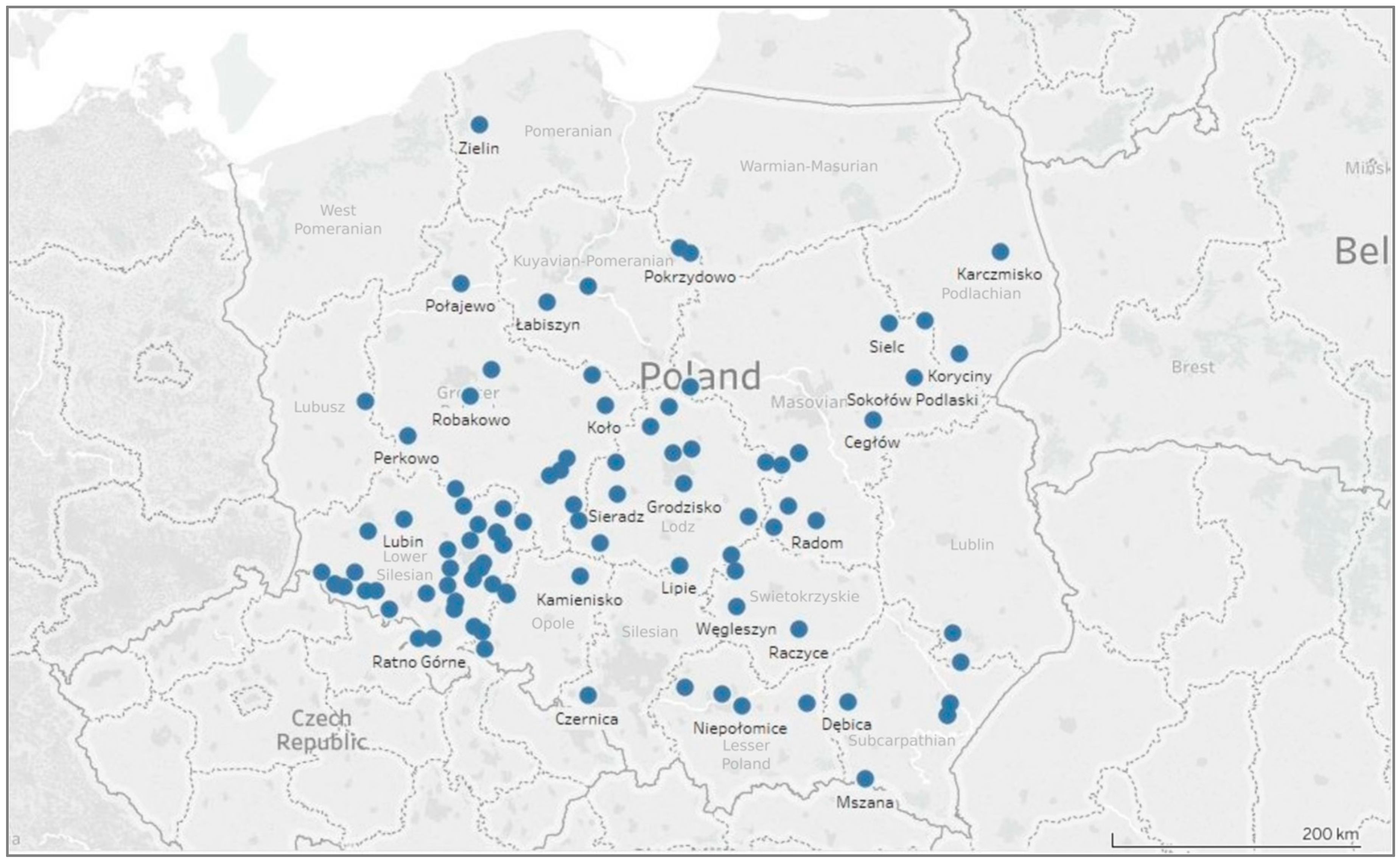
2.2. Analysis Database

The research used data on producers of unprocessed food (i.e., vegetables, fruits, meat, eggs, etc.) that was collected from available public databases (exhibitor lists of food producers published on the official website of the marketplace i.e., Targpiast marketplace, Lower Silesian Center of Agricultural and Food Wholesale Market—LSCAFWM). Information obtained from these lists was updated according to the national court register, data obtained from food producers (through questionnaires sent out by email and/or, if available, via food producers’ websites), and data obtained from field research conducted at marketplaces and bazaars in Wrocław. We also took into account the food suppliers of the “Lokalny rolnik” (Local farmer) initiative, which delivered organic food for organized purchasing groups in Wrocław. The data were collected from April to October 2017 (Table 1—the symbol “x” showed the source of data collection for given bazaar or marketplace). In our study, we considered only national products, which is connected with the idea of foodshed assessment. The foodshed analysis is a local approach, which is in opposition to a global food system. It represents the local food zone for urbanized areas.
The study also used data representing the spatial boundaries of administrative units, which was acquired from the Center for Geodetic and Cartographic Documentation.

2.3. Determining the Framework of Data Analysis

The data obtained from each of the sources allowed us to build our database, which consisted of information such as the name of the bazaar/marketplace/initiative, name of the producer, address of the company, place of food production by company, and the names of the products produced by each company. The next step of building the database was to assign each product to a group of products according to the food groups mentioned in the food basket [46]. Food baskets were determined for each European country within the European Reference Budget Network project financed by the European Commission. Therefore, products were divided into six product groups based on the healthy food pyramid: (1) cereal products; (2) vegetables and tubers; (3) fruits; (4) milk and milk products; (5) meat, fish, eggs and legumes; and (6) fats [46].
The preparation of data allowed us to conduct a database analysis using the Tableau Software (Version 10.5), which could be integrated with data from other programs [47], in this case with Dell Statistica—Data Analysis System (Version 13). Firstly, we prepared an analysis of food producers’ locations. Secondly, we analyzed the number of products produced in each localized place. Thirdly, we assigned each product to a group of products based on the healthy food pyramid, and analyzed these groups according to regions (in Poland—voivodeships). We also decided to perform a statistical analysis of the relationships between product groups and the voivodeships from which they originated, using the chi-square test. Then, we carried out an analysis of a group of products defined on the basis of a food pyramid, differing by the distance from the origin of the products, using the non-parametric ANOVA test by Kruskal–Wallis. Furthermore, we conducted an analysis of products clustering according to the distance of their origin, using the k-means clustering method. We decided to use the k-means clustering method, and therefore a non-hierarchical method rather than a hierarchical model, because of its time complexity, which is “linear in the number of documents” [48]. Furthermore, the k-means clustering method improves the hierarchical clustering by non-mixing nearest neighbors in the same clusters, which is not the case when using hierarchical methods, even at the earliest stage of clustering [48].

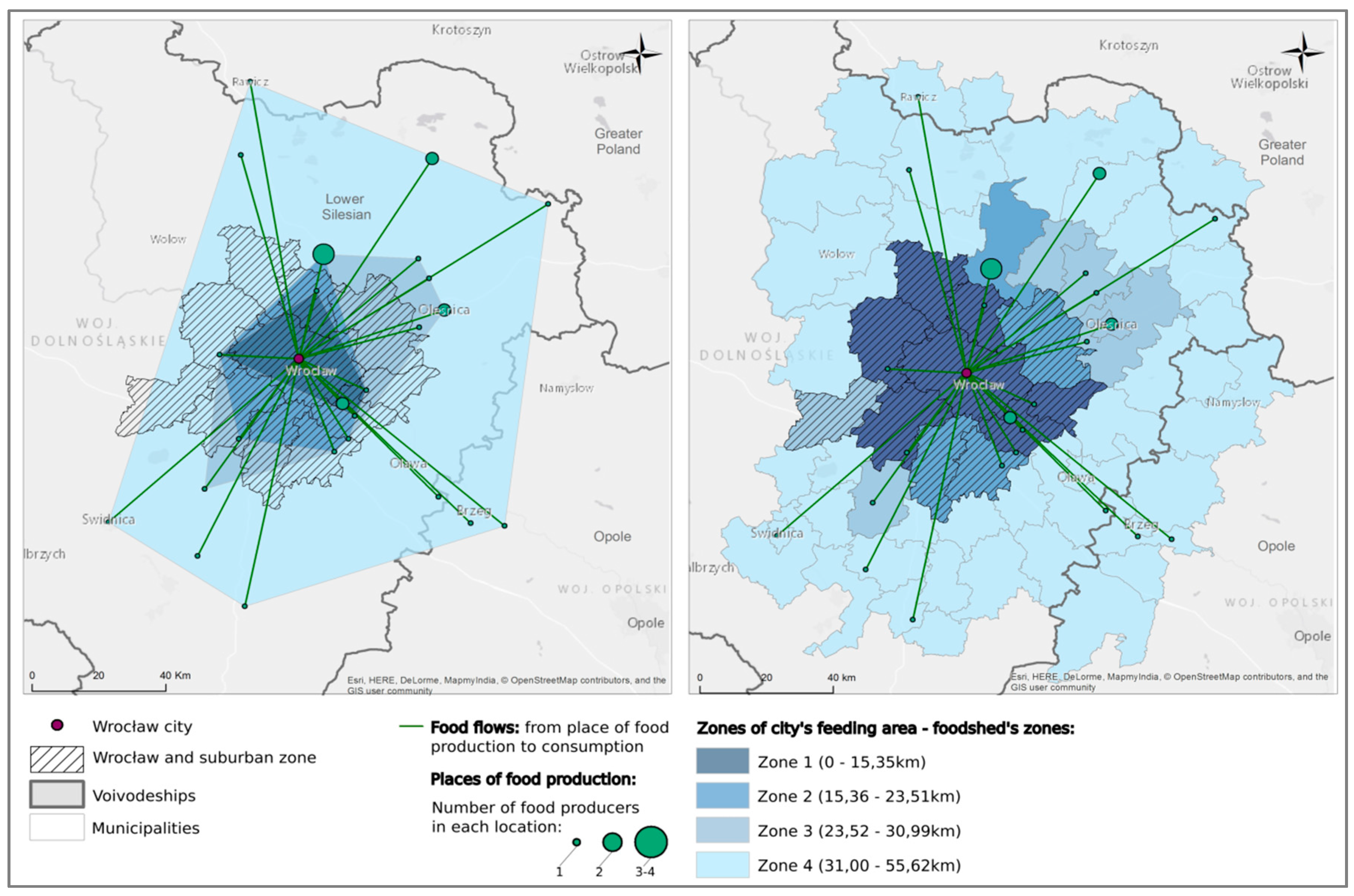
2.4. Determining a Framework of Foodshed Assessment

Existing research on foodshed determination is based on information regarding food flows between the places of production and consumption [33]. The first step of the analysis was to prepare and compile the collected data into a ‘csv’ file. Then, we had to geocode the data, representing places of food production as point vector data using the ArcGIS Online platform. Vector data were the basis for generating food flows between places of food production and the city of Wrocław: the place of its consumption. The lines representing the flows of food were generated using the Construct Sight Line tool from ArcGIS Software (Version 10.4.1).
The next step of the analysis was a geometric calculation to estimate the distance of each connection. This allowed us to divide the calculated distances into classes according to the natural distribution by using the graphical method (which is the same method used in the work of Karg et al. 2016). The first data class (representing the objects closest to the city) represented the objects that enabled mapping the minimum boundary of the city’s foodshed. We mapped this boundary using the Minimum Bounding Geometry tool (Convex hull option). Then, the use of spatial query (selection by location tool according to intersect—i.e., the spatial selection method) allowed us to construct the administrative boundary of the city’s foodshed based on the intersections between the areas of the minimum foodshed boundary—which was designated using Convex hull—and the municipalities’ administrative borders (Figure 2).
Moreover, we decided to expand the framework of foodshed determination through the delimitation of a city’s foodshed zones. Therefore, the data class that represented the distances of the city’s foodshed boundary was divided. The division was made again using the graphical method. Then, we mapped the minimum boundaries of the city’s foodshed zones using the Minimum Bounding Geometry (Convex hull option) and selection by location in order to determine their administrative boundaries. This solution was a base to verify the obtained boundaries of the city’s foodshed zones according to the city’s suburban zones.

3. Results

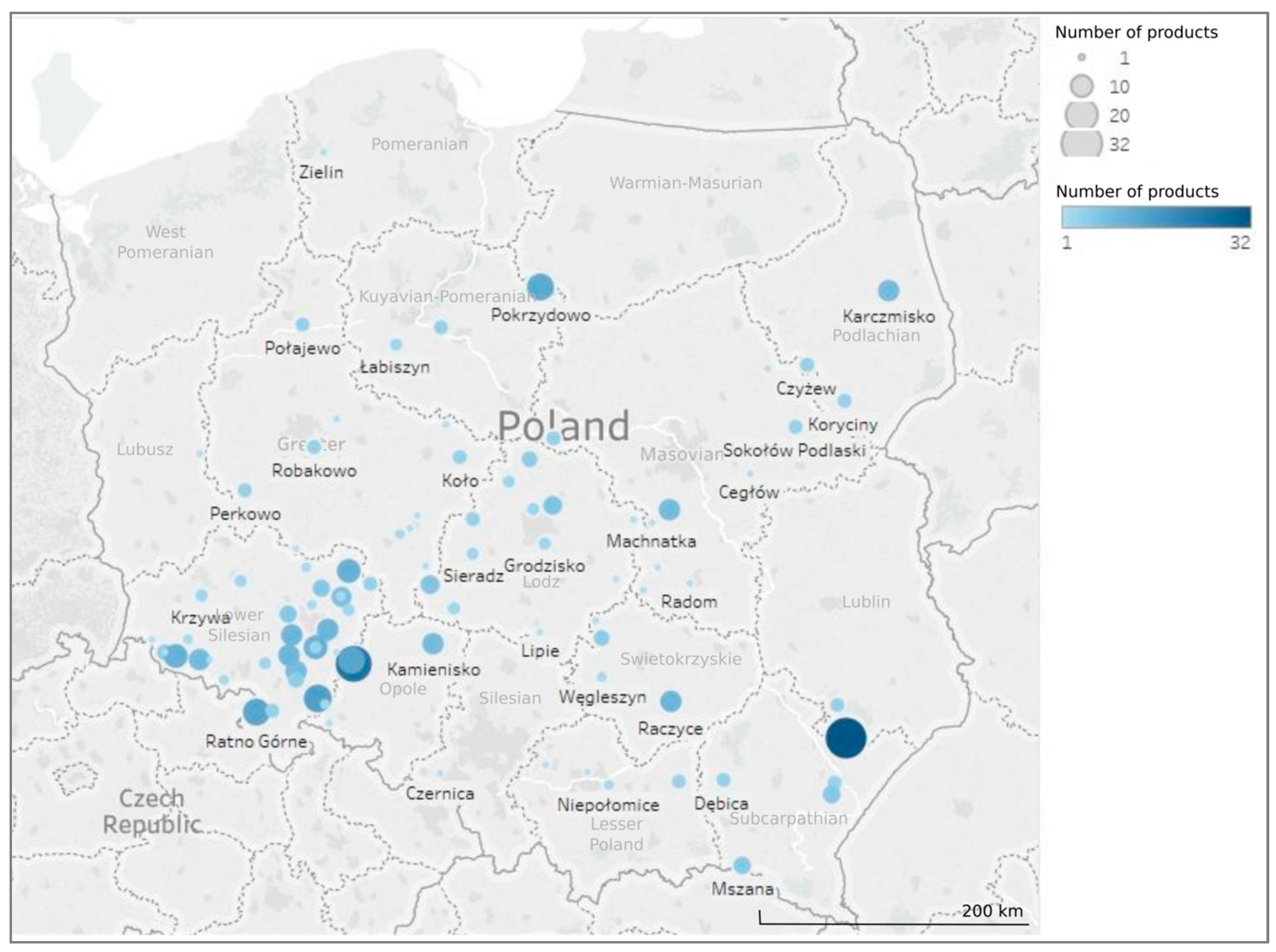
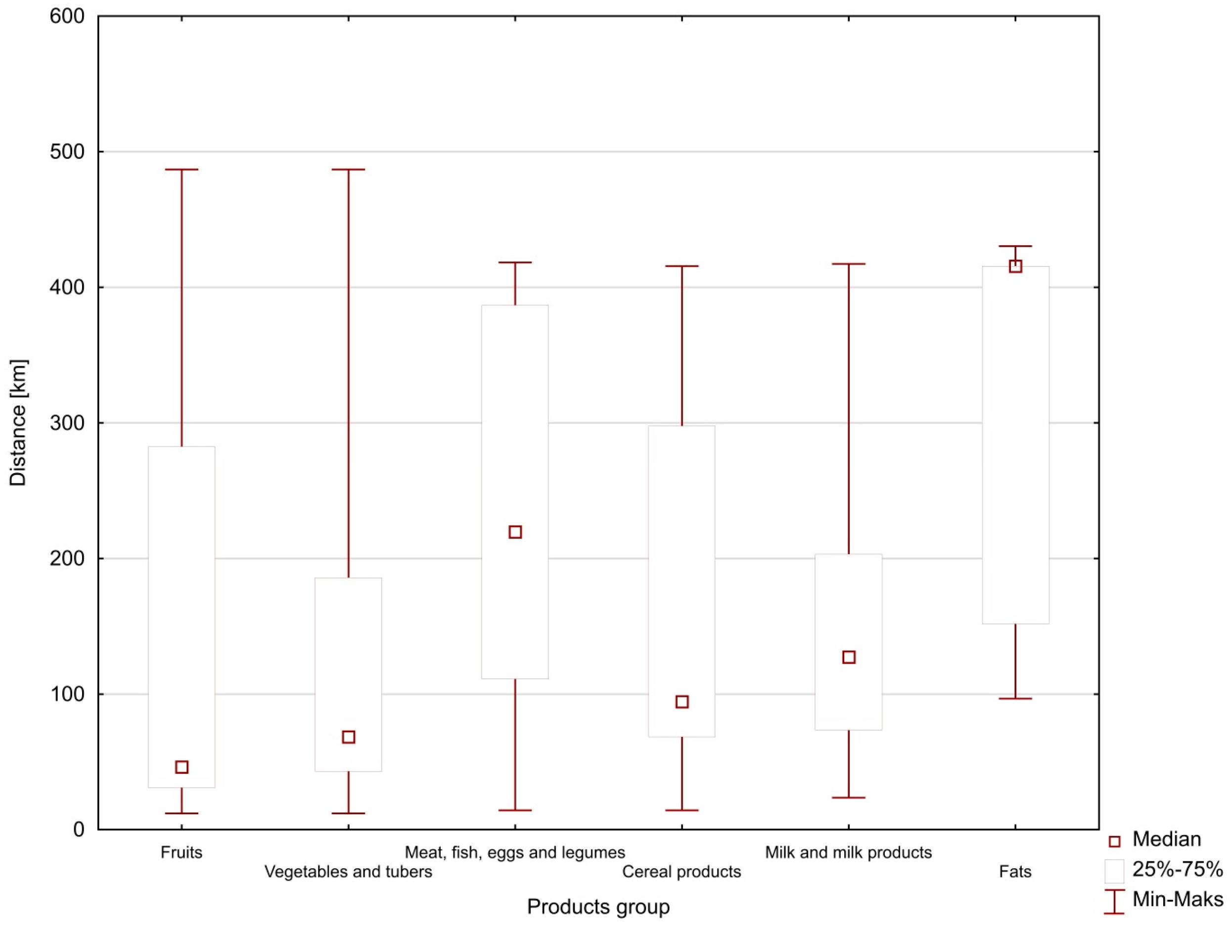
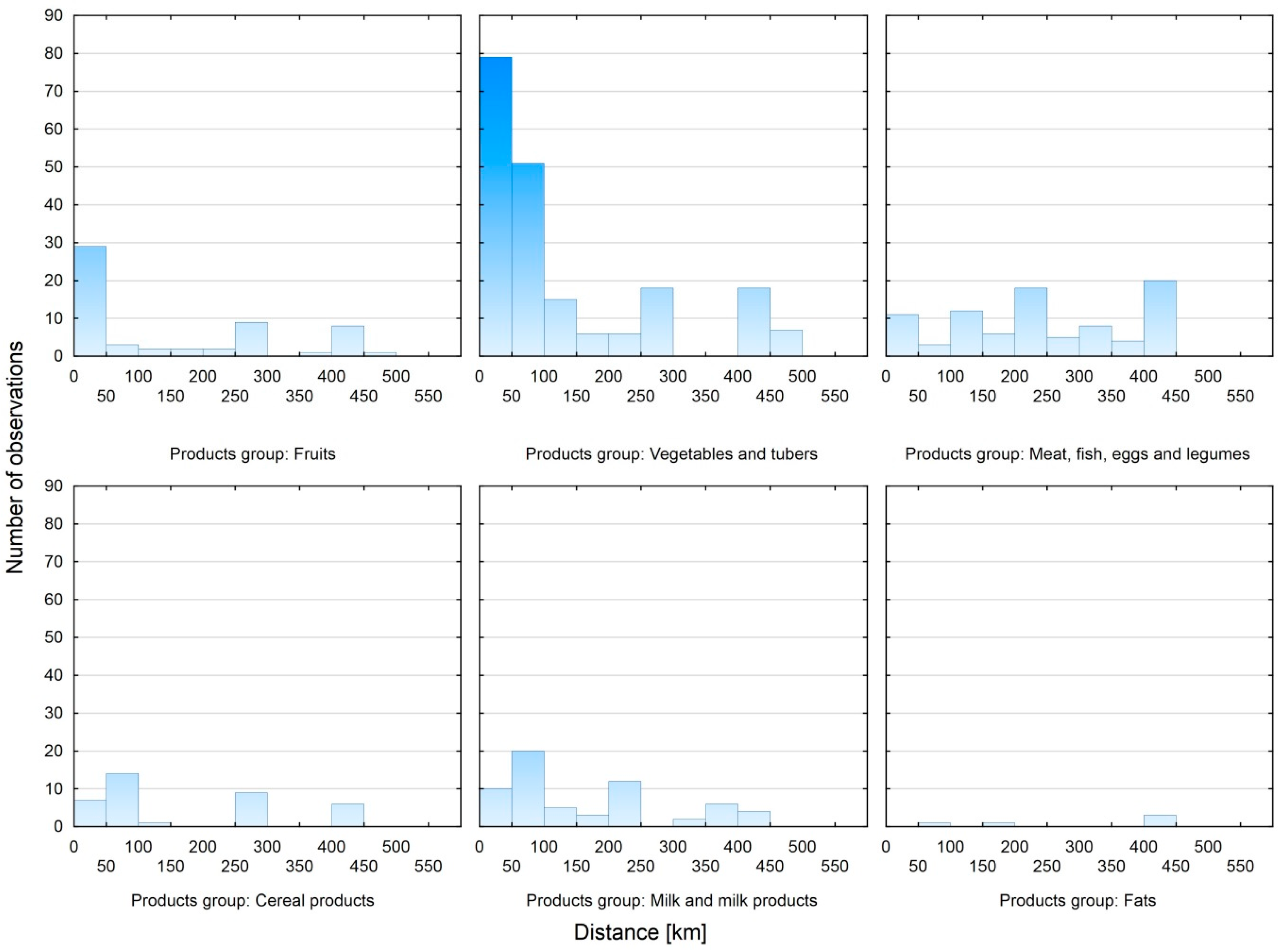
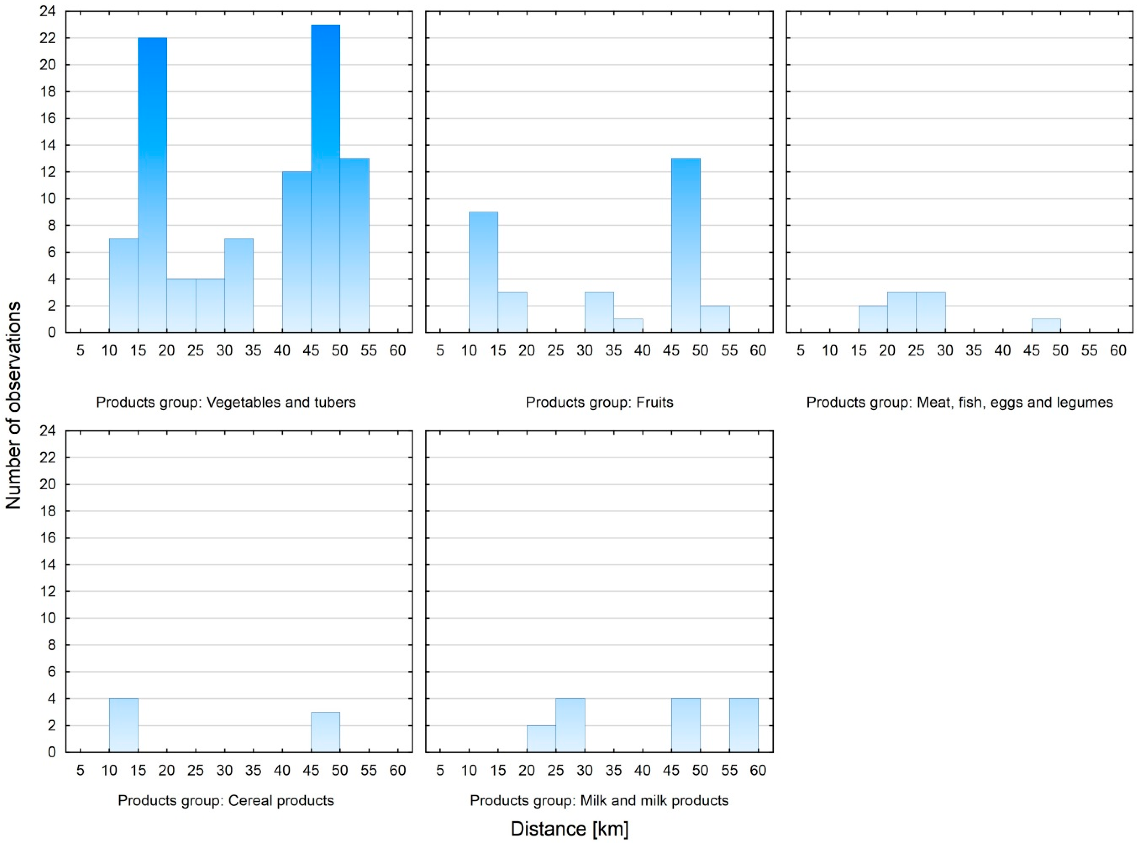
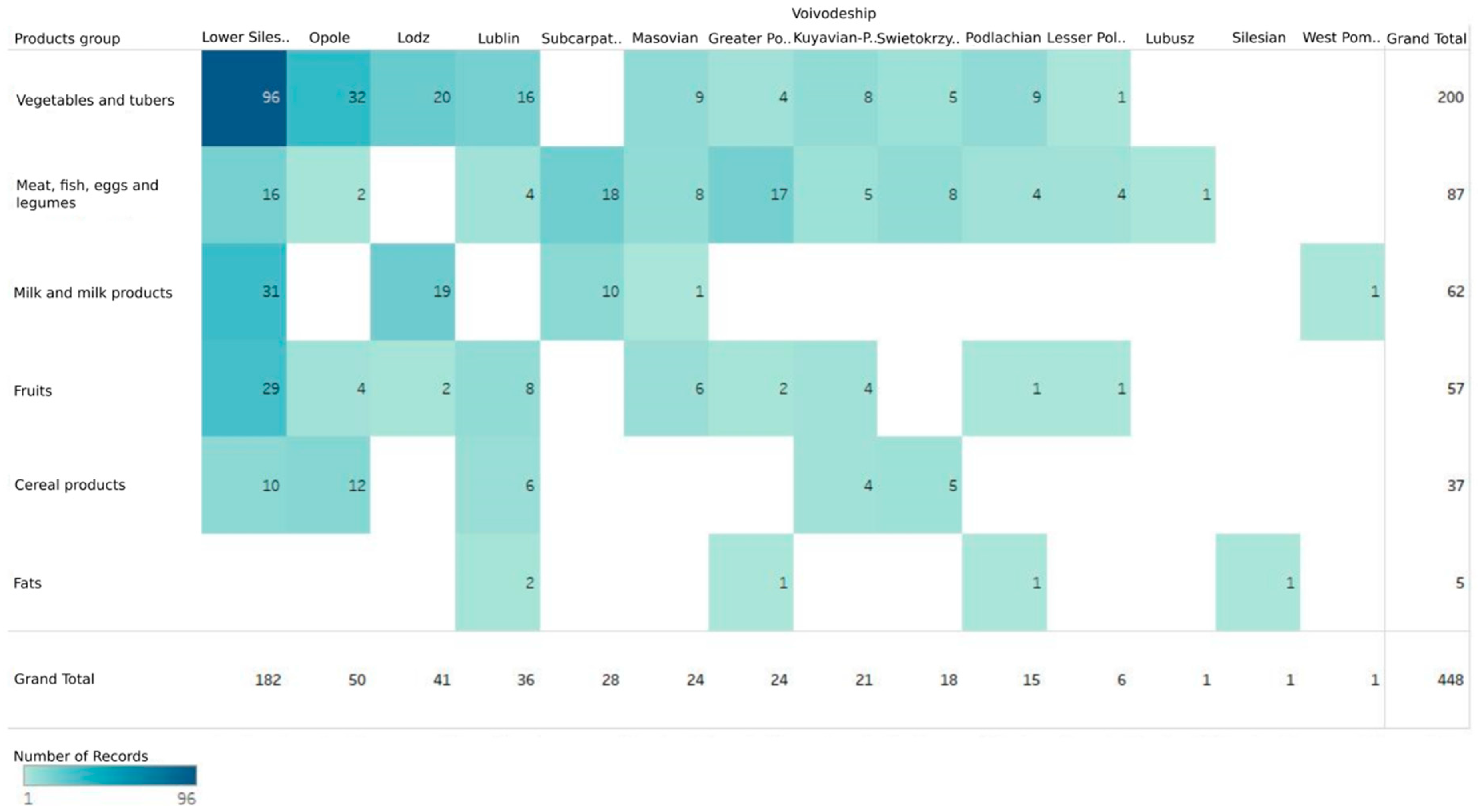
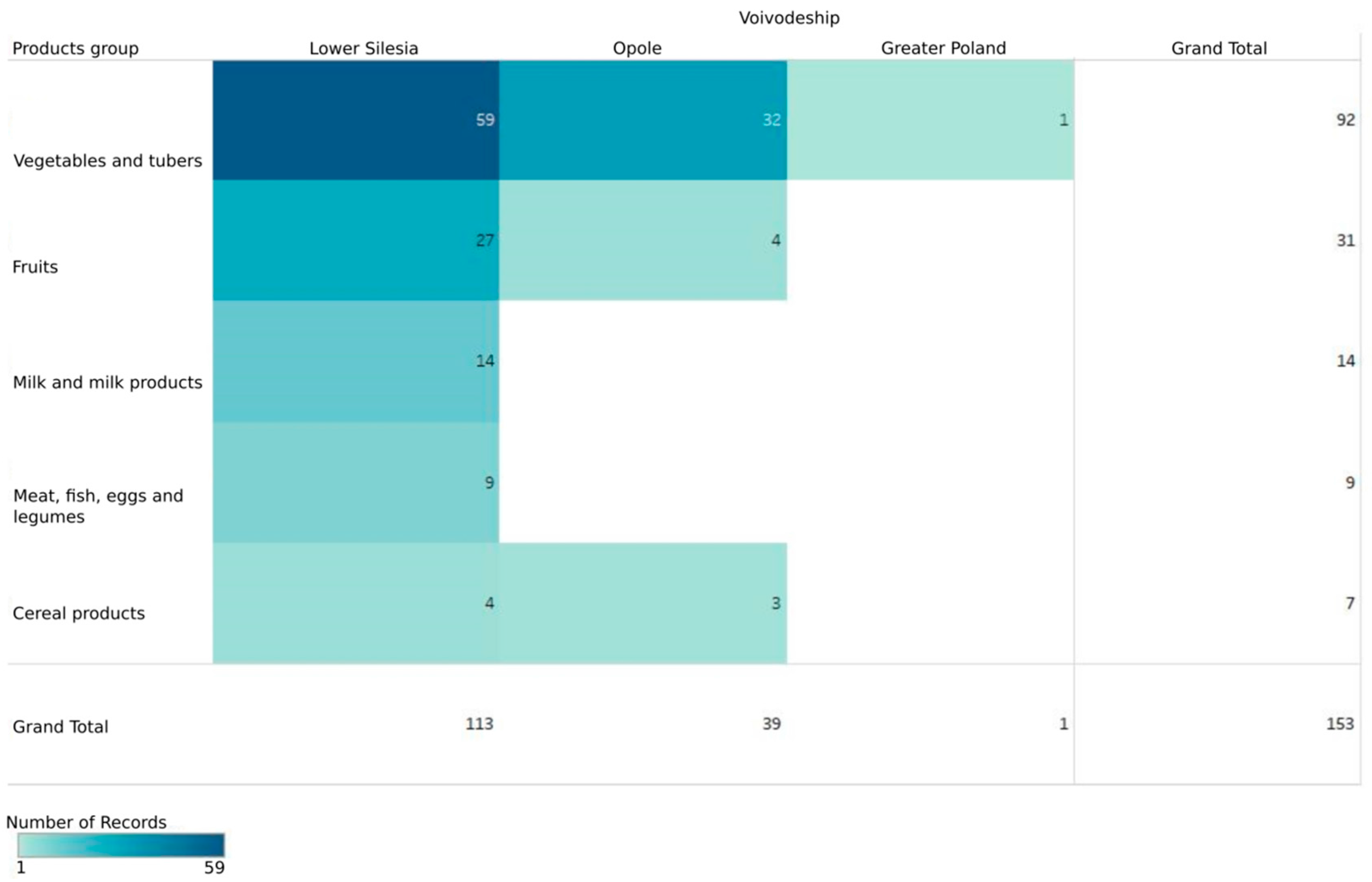
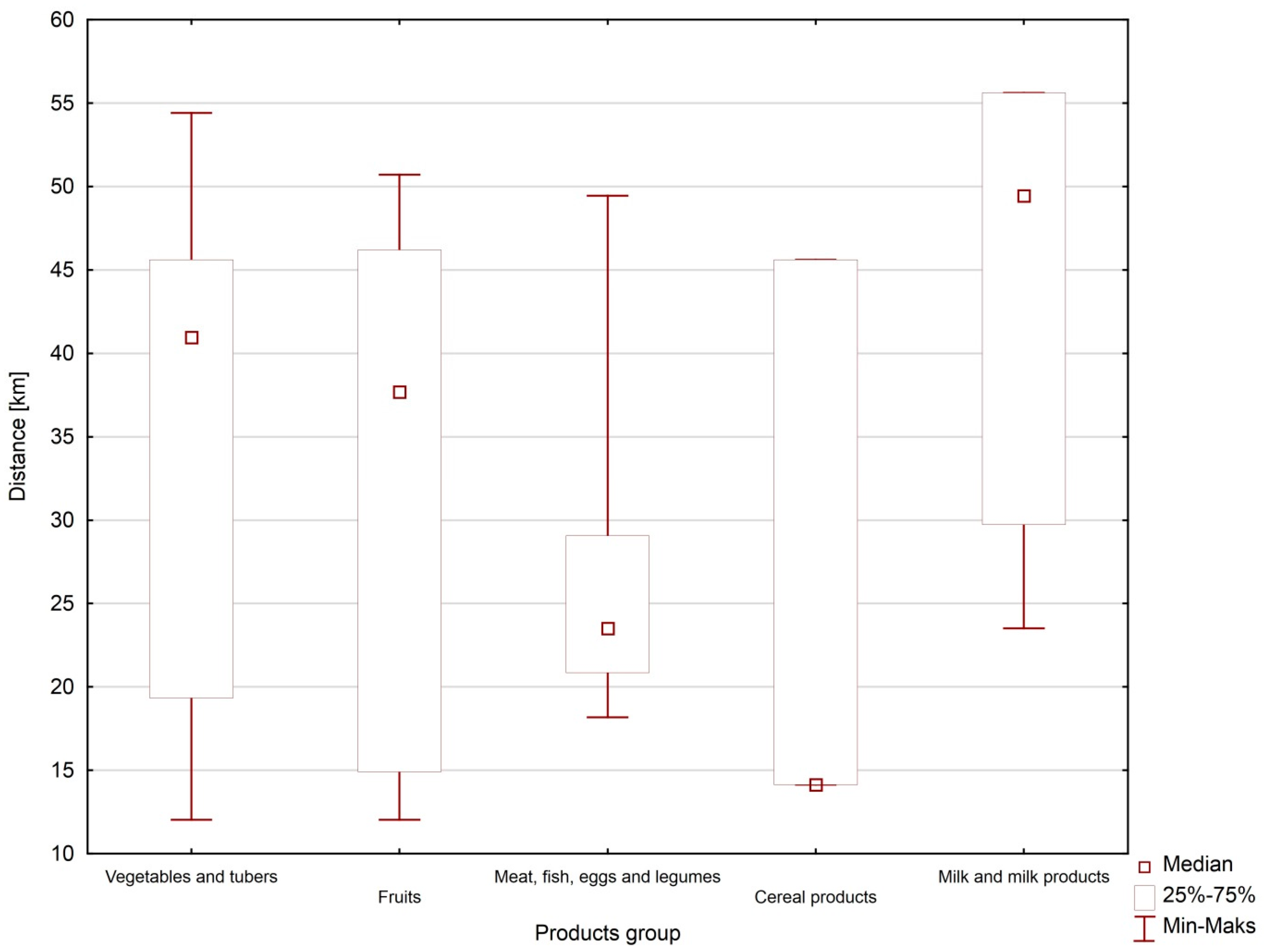
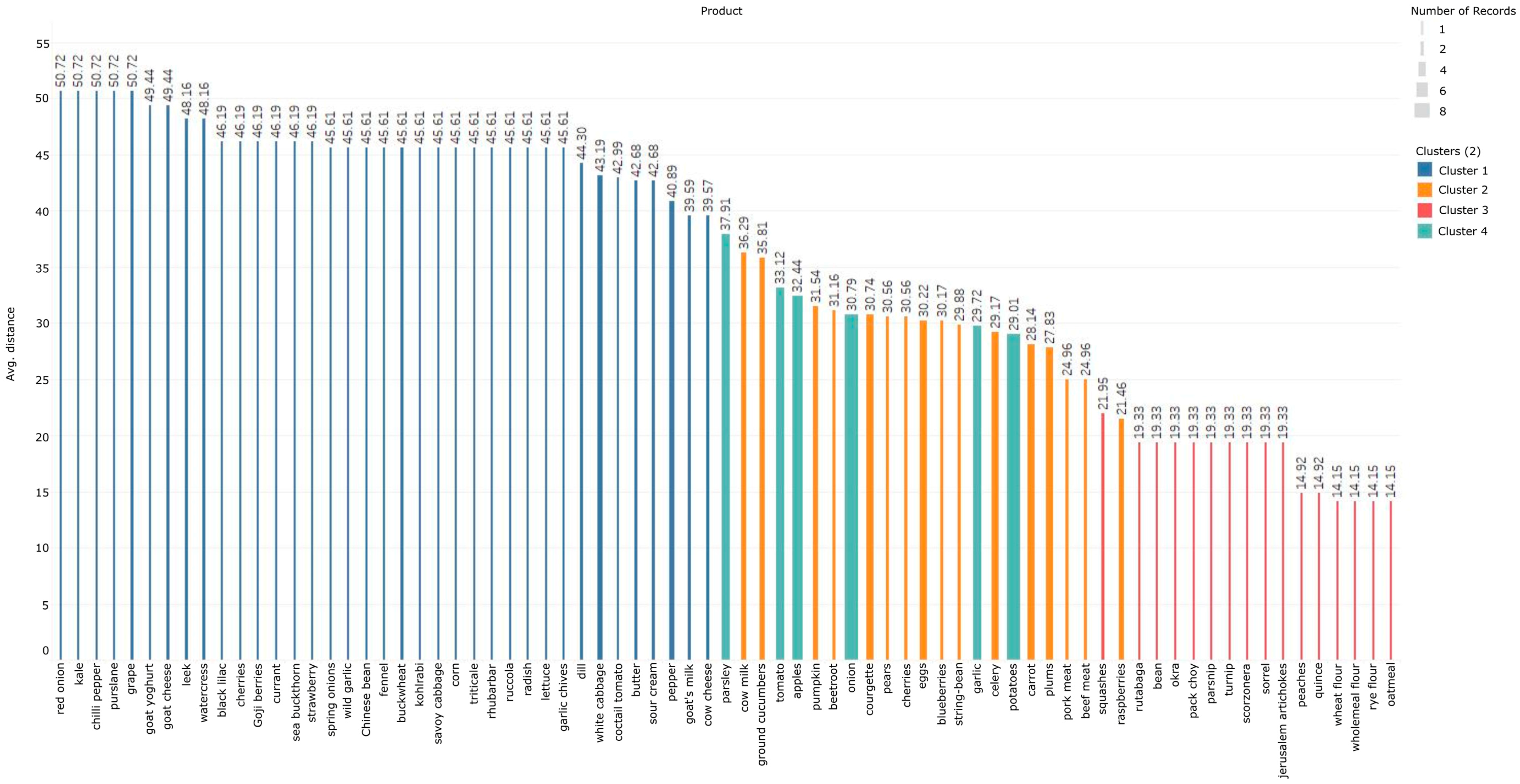
3.1. Data Analysis Results

In our research, we obtained information about 448 products that were available at Wrocław bazaars and markets. We counted and categorized those products according to their type, and thus obtained 115 types of products (e.g., potatoes, broccoli, cow cheese, barley flakes, etc.). We noticed that national products came from 98 places (more often from villages than towns) (Figure 3).
The food products available at the marketplaces and bazaars in Wrocław were most often produced in the Lower Silesian Voivodeship. This indicates that the southwestern part of Poland had the largest concentration of product locations. This concentration of production places extended from the southeastern part to the central part of the country. The lowest concentration of food production places was seen to the east of the Lower Silesian Voivodeship: Opole, Silesia, Lesser Poland, and the entire eastern part of the country (from southeastern to northeastern: Subcarpathian, Lublin, Podlachian). A decrease of concentration in food production places was also observed west of the Lower Silesian Voivodeship (Lubusz). We made no observations in the north of Poland (Warmian-Masovian) and in the northwestern part of the country (West Pomerania).
Although the eastern part of the country was characterized by the smallest number of food production places, the largest number of food products was recorded in Tarnogród (Lublin Voivodeship): 32 of the products that were available at the analyzed Wrocław marketplaces and bazaars. The next largest number of products was noted in the Opole Voivodeship (to the east of Lower Silesia), in Żłobizna village. In this area, the recorded number of food products was calculated as 25 products. Other places with the largest number of products were localized in Lower Silesia, at the level of 15 products in Lubnów (near the border of the Opole Voivodeship), and also in Ratno Górne village (near the border with the Czech Republic)—at the level of 14 products. We noted also 14 food products in the Opole Voivodeship—in Kruszyna village (near the border of the Lower Silesian Voivodeship), and 13 products in the Kuyavian-Pomeranian Voivodeship, in Pokrzydowo village (Figure 4).
Having obtained information about the places and the numbers of products produced in each location, we decided to prepare a matrix for the regions (voivodeships) based on the groups of products defined within the framework of the healthy food pyramid. Therefore, we obtained the information that 182 out of the 448 food products were produced in Lower Silesia, 50 products came from Opole, 41 came from Lodz, and 36 came from Lublin. Less than 30 food products were produced in regions such as the Subcarpathian, Masovian, Greater Poland, Kuyavian-Pomeranian, Swietokrzyskie, Podlachian, Lesser Poland, Lubusz, Silesian, and West Pomeranian. Moreover, we classified: 200 products as vegetables and tubers; 87 products as meat, fish, eggs and legumes; 62 products as milk and milk products; 57 products as fruits; 37 products as cereals; and five products as fats (Figure 5).
The largest number of products in each product group were produced in Lower Silesia. Furthermore, out of the 182 that were produced in Lower Silesia, we classified: 96 products as vegetables; 31 products as milk and milk products; 29 products as fruits; 16 products as meat, fish, eggs and legumes; and 10 products as cereals. There were no producers of fats in Lower Silesia. The region with the second largest number of food products for Wrocław was Opole. This circumstance could be understood because of the close proximity of these two regions. What could be astonishing is that the next four regions with the largest number of produced food products are not situated the closest to Wrocław or Lower Silesia, which could be connected with the spatial distribution of food production sites (as on Figure 3). Moreover, Greater Poland, which is the neighboring region with Lower Silesia, is only in the sixth position in the prepared ranking (Figure 5).
Therefore, we decided to analyze the relationship between the product groups and the voivodeships from which they came. The chi-square tests for categorical (qualitative) variables did not find application because of the limited use of the test; the expected frequencies in the cross-tabulation tables were too small.
Furthermore, we conducted a non-parametric Kruskal–Wallis ANOVA test for product groups in terms of the product’s distance of origin. The test showed a statistically significant difference between groups of products (H (5, N = 448) = 45.47 p = 0.00). The box and whiskers plot for distance depending on product group were presented on Figure 6.
Moreover, we prepared histograms of distance depending on the product group. These analyses showed (Figure 7) that most of the Vegetable and tuber products—ca. 80, were delivered up to a 50-km distance, and ca. 50 products were delivered within 50–100 km. The fruit group, ca. 30 products, had the highest proportion of its products delivered within 0–50 km.
Most of the products in the Meat, fish, eggs and legume group were delivered within the ranges of 400–450 km and 200–250 km. The Cereal products group had the largest number of products delivered within 50–100 km: ca. 15. The Milk and milk products group had 20 products delivered within 50–100 km, and ca. 12 products delivered within 200–250 km, which represented the largest number of products delivered within this product group. Finally, the Fats group had the largest number of products delivered within 400–450 km.
The last results that we obtained using the Tableau Software allowed us to analyze the data according to distance between food production place and consumption destination. This analysis was made for each product according to its average distances, using the K-means clustering method. This analysis allowed to verify how the data could be clustered in the context of foodshed boundary designation. We obtained four clusters: 55 food products were classified in the first cluster (14.2–94.4 km), 31 products were classified in the second cluster (119.6–211.2 km), 20 products were classified in the third cluster (216.1–297.8 km), and nine products were classified in the last cluster (347.8–415.6 km). The ‘Vegetables and tubers’ group accounted for 32 of the 55 products in the first cluster; these included: red onion, chives, garden cress, red potatoes, courgette, parsnip, chilli pepper, kale, ruccola, cocktail tomato, purslane, watercress, fennel, Chinese bean, wild garlic, spring onions, sorrel, scorzonera, turnip, rutabaga, squashes, Jerusalem artichokes, dill, garlic chives, lettuce, radish, potatoes, red cabbage, savoy cabbage, and kohlrabi. “Cereals” was the second-largest group in the first cluster, with 11 products: wheat flakes, rye flakes, spelt flakes, barley flakes, barley flour, buckwheat flour, oatmeal, wholemeal flour, triticale, corn, and buckwheat. The “Fruits” group had nine products in the first cluster: plums, grape, sea buckthorn, Goji berries, black lilac, quince, peaches, blueberries, and rhubarb. The groups that were least represented in the first cluster were: “Meat, fish, eggs and legumes”, which only had two products (lamb and veal), and “Milk and milk products”, which only had one product (goat yoghurt). The most commonly available product in this cluster was potatoes, which was recorded 18 times (Figure 8).
The second cluster represented 31 food products. The main food group in the second cluster was “Vegetables and tubers”, with 13 products: white cabbage, onion, celery, tomato, leek, garlic, bean, beetroot, parsley, carrot, pumpkin, ground cucumbers, and string bean. The second most represented group in the second cluster was “Milk and milk products”, with eight products: cow cheese, butter, goat milk, goat cheese, cow milk, natural yogurt, kefir, and sour cream). The third largest group of food products was ‘Fruits’, which had four products: cherries, raspberries, pears, and apples). The final two groups had three food products each; the “Cereals” in the second cluster included rye flour, wheat flour, and spelt flour and the “Meat, fish, eggs and legumes” were eggs, rabbit meat, and duck meat). The most frequently noted products in the second cluster were onion (20 times), apples (19 times), garlic (17 times), and cow cheese (15 times). Furthermore, it could be seen that in the first and second cluster, which end with a distance of 211.2 km, there were no “Fats” products.
There were a total of 20 products in the third cluster. The largest number of products were in the “Cereals” group, which had six food products: buckwheat, corn groats, fine-milled buckwheat, small spelt, wheat, and spelt. The second-largest group in the third cluster was “Vegetables and tubers”, with five products: pepper, green lentils, red lentils, soy, and pea. The third-largest group in the third cluster was the “Meat, fish, eggs and legumes” group, with four products: sausages, beef meat, pork meat, and poultry. The last two food groups of products in this cluster were “Fruits” (strawberry, currant, and cherries) and “Fats” (organic oils), which made its first appearance in the clusters with an average distance of 226 km. Honey also appeared in this cluster, which could not be classified into any specific group. The products that were noted most often in the third cluster were sausages (19 times), beef meat (18 times), pork meat (17 times), and poultry (17 times).
The last and final cluster contained nine products. The most representative group was “Vegetables and tubers”, with three products: cauliflower, broccoli, and spinach). The next three food groups had two products each: “Fruits” (chokeberry and gooseberry), “Cereals” (barley and millet), and “Fats’ (rapeseed oil and linseed oil). An analysis of all of the clusters and products revealed that vegetables and fruits were the most available products. The group of food products that were not available locally was “Fats”, which were imported from an average distance of 226 km. Obtained data provided a base for the determination of the city’s foodshed.

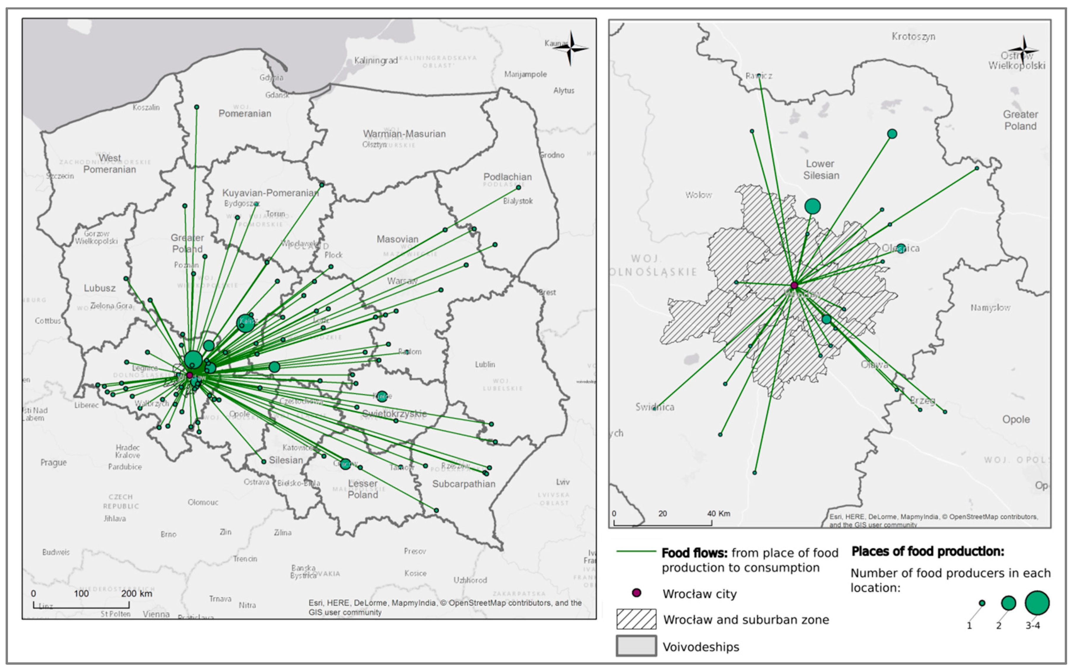
3.2. Foodshed Boundary Determination

The geocoding of the data allowed us to visualize the places of food production, which in turn determined the flow of food from the place of its production to Wrocław (Figure 9).
The data allowed to designate 98 places of food production that sent products to the bazaars and markets in Wrocław. Furthermore, we divided the data into classes according to the products’ natural distribution, using the graphical method. The distribution of data allowed us to designate 24 food production places, which were the basis for determining the foodshed of Wrocław. Some places, such as Trzebnica (in Lower Silesia), Kalisz (in Greater Poland), Oleśnica, and Radwanice (in Lower Silesian) were characterized by more than one food producer. Therefore, Wrocław’s foodshed boundary was determined based on food that originated from Lower Silesia, but also with bordering regions such as Greater Poland and the Opole Voivodeship. This was related to the designated value of distance, which extended to 55.62 km. Moreover, we spread the foodshed assessment, and divided the obtained distance data into zones of the city’s foodshed.
We designated two boundaries of the Wrocław foodshed. The first method allowed us to map the minimum boundary of the foodshed using the Minimum Bounding Geometry tool, which delimitated the foodshed boundary with an area of 5663 km2. The second method, which joined the obtained area within the spatial link with municipalities, delimitated the administrative boundary of foodshed within 8871 km2, and mainly covered the area of Lower Silesia. The municipalities of the Opole and Great Poland regions represented a smaller share of the total area. The coverage of the foodshed extended beyond the municipalities of Wrocław (i.e., its suburban zone), and spread up to 56 km. The nearest zones—I and II—represented almost all of the neighboring communities of Wrocław. Zone I contained six out of Wrocław’s 10 suburban municipalities as the nearest foodshed area, while zone II contained three suburban municipalities, and only one of the 10 suburban municipalities was classified into zone III. Apart from Wrocław’s suburban municipalities, other municipalities were also classified within zones I, II and III. The second zone also included Trzebnica (north of the Wrocław suburban zone). The third zone included such communities as Sobotka (southwest of the Wrocław suburban zone), Zawonia, Dobroszyce, and Oleśnica (northeast of the Wrocław suburban zone) (Figure 10).
The delimitated foodshed area allowed us to classify 153 products from 24 food producers (Figure 11). The products were categorized according to five of the six food product groups. Products from “Fats” were not identified. The highest percentage of products came from Lower Silesia (approximately 74% of the total), while 25% came from Opole region, and less than 1% came from Greater Poland. The greatest availability was noted for the “Vegetables and tubers” group, which represented 60% of all of the food products within Wrocław’s foodshed area. The next group, “Fruits”, represented 20% of all of the products. Of the final three groups, “Milk and milk products” represented 9% of the total food products, while ‘Meat, fish, eggs and legumes’ made up 6%, and “Cereals” made up approximately 5%.
The chi-square test (verifying the relationships between product groups and the voivodeships from which they originated) for data representing the designated area of the city’s foodshed was also not applicable, due to its restrictions.
Another analysis, the Kruskal–Wallis ANOVA test, showed a statistically significant difference between groups of products (H (4, N = 153) = 10.60, p = 0.03). Multiple (bilateral) comparisons showed that products from the “Cereals” group were transported a smaller distance than products from the “Milk and milk products” group. A box and whiskers plot for the analysis is shown in Figure 12.
Histograms of distance depending on the product groups for the Wrocław foodshed zone (Figure 13) showed that the Vegetables and tubers products were most often delivered distances of 45–50 km and 15–20 km. Most of the products within the Fruits group were also delivered within 45–50 km, as in the case of Vegetables and tubers. However, the ‘Fruits’ group also delivered a high amount of its products within a distance of 10–15 km. Most of the Meat, fish, eggs and legumes products were delivered within 20–25 km and 25–30 km. Most of the products within the ‘Cereals’ group were delivered within 10–15 km. It could be worth mentioning that the second and last distance of origin for Cereal products was within 45–50 km. This could show that cereal products are delivered mainly from the closest and farthest areas of the designated foodshed zone. There was a lack of these products within a distance range of 15–45 km. The group with the highest number of products from three distances, i.e., 25–30 km, 45–50 km, and 55–60 km, was the Milk and milk products group. The closest distance, up to 5 km, was not noticed in any of analyzed products groups.
We also clustered the data using the k-means clustering method. This time, the homogeneous clusters were not seen, as it was within the context of all of the analyzed data (Figure 14). The analyzed data allowed us to verify 75 food products. The obtained classification showed that 16 products were classified in the first cluster; these products were primarily “Vegetables and tubers”, such as: squashes, Jerusalem artichokes, sorrel, scorzonera, turnip, parsnip, pak choy, okra, rutabaga, and bean. In the earlier analysis for all of the data, the average distance was ca. 150 km, and for the city’s foodshed, the average distance was ca. 15–20 km. The second-largest group of products in the first cluster was “Cereals”, with four food products: oatmeal, wholemeal flour, rye flour, and wheat flour. The comparison of data obtained for the Wrocław foodshed area with all of the data showed that rye flour and wheat flour minimized the average distance from ca. 150 km to ca. 15 km. The next and the last group of products within this cluster was “Fruits”, which included quince and peaches.
The second cluster, for which distances were ca. 20 and 38 km, was also dominated by the “Vegetables and tubers” group, with eight food products: carrot, which changed distance from 80 km to 30 km, celery, string bean, courgette, beetroot, pumpkin, ground cucumbers, and parsley, which changed distance from 150–200 km to ca. 30–35 km. The next largest group, which had five products, was “Fruits”. Earlier distances were: 120 km for raspberries, ca. 82 km for plums, 230 km for cherries, and 190 km for pears, while the distance did not change drastically for blueberries. The second cluster also included three products within the “Meat, fish, eggs and legumes” group: beef meat, pork meat, and eggs. These products also changed their average distances at the local scale, which was earlier calculated as 160 km for eggs and 250 km for beef and pork meat. The last product classified in this cluster was cow milk from the “Milk and milk products” group, for which distance decreased from 180 km.
The third cluster (30–40 km) was dominated by five products: four “Vegetables and tubers”, and one product from the “Fruits” group. These groups included products that had earlier been classified within much larger distances: potatoes had an average distance of 88 km beforehand; while garlic was ca. 159 km, onion was ca. 130 km, tomato was ca. 140 km, and apple was ca. 190 km.
The fourth cluster had a distance ca. 40–50 km, and contained 37 food products: 20 from the “Vegetables and tubers” group, eight from the “Fruits” group, six from the “Milk and milk products” group, and three from the “Cereals” group. The “Vegetables and tubers” included: pepper, cocktail tomato, white cabbage, dill, garlic chives, lettuce, radish, ruccola, savoy cabbage, kohlrabi, fennel, Chinese bean, wild garlic, spring onions, watercress, leek, purslane, chilli pepper, kale, and red onion. There were also some products for which the average distance decreased: pepper decreased from 230 km, leek from 145 km, cabbage from 120 km, and red onion from 65 km. Other products could be marked as local, because in each case, the average distance for them was similar or the same, ca. 45–50 km. The second-largest group of products within the fourth cluster was “Fruits”, with eight food products. The fruits within this cluster included: rhubarb, sea buckthorn, Goji berries, black lilac, and grape, all of which were classified in the same cluster according to average distance. Therefore, these food products could be marked as local, or in other words, products that are available in the foodshed of Wrocław. Other fruit products were reclassified, and according to this new classification, their average distance changed. These fruits included strawberry (average distance decreased from 216 km), currant (from 230 km), and cherries (from 230 km). The next largest group within the fourth cluster was “Milk and milk products”, which included: cow cheese, goat milk, sour cream, butter, goat cheese, and goat yogurt. All of these products decreased their average distance in comparison with the general analysis (cheese, butter, and goat milk all decreased from 130–145 km to ca. 50 km; goat yogurt decreased from 93 km; cow cheese, butter, and goat milk decreased from 130–145 km; goat cheese decreased from 180 km, and sour cream decreased from 205 km). The last group in the fourth cluster was “Cereals”, with three food products: triticale, corn, and buckwheat. These products did not change their average distance in comparison to the general data.
The products that were represented within the city’s foodshed boundary were 34% of all noticed products in our research. The designated area was created on the basis of 25% of the data representing places of origin for the food products that were available at the bazaars and markets in Wrocław. This means that as much as 75% of the places of origin for the food in Wrocław exceeded the area of the food supply zone, which was calculated as 55.62 km.

4. Discussion

Nowadays, analyses in the context of satisfying the needs of the local community are important [49,50]. This is especially important because in the context of population growth [51], resources become limited [21] and the environmental carrying capacity is exceeded [52], which leads to negative impacts on the environment [53] and an upset in its natural balance [54]. Therefore, conducting environmental analyses could provide information about resource capacity, limits, and when these are exceeded [55], and thus help determine goals for resource management [56]. The foodshed analysis and the related problem of food miles highlights the connections between the geographical boundaries of a food system and the need to promote environmental sustainability [57]. Therefore, the need for conducting foodshed analysis is still valid. In fact, the need for an analysis of food systems at a local level is more important than ever, because food systems are becoming more regional [58] or even global [59], and thus the use of land and resources is no longer sustainable [59]. In view of the above, the use of foodshed analysis is an important element for plans and strategies for improving sustainability and evaluating the capacity to localize food production [60]. These aspects could be useful for creating regional development strategies. As Lengnick et al. (2015) wrote, the implementation of foodshed analysis into strategies allows researchers and policymakers to “redefine the relationship between urban and rural areas [and] recognize the potential for food systems to address shared challenges such as securing clean water supplies, conserving biodiversity, mitigating global warming, and cultivating climate resilience” [61].
Most foodshed assessment methods determine the boundary of foodsheds by the buffer from the city [39] or according to administrative units [38]. We determined the extent of the food zone based on the relationships between places of food production and its consumption, which reached 55.62 km. Therefore, if we would like to calculate the buffer of Wrocław’s food zone, it could be defined as an area of ca. 3094 km2. The foodshed zone area that we calculated using the Minimum Bounding Geometry tool was 5663 km2, and using spatial query, the administrative boundary of the foodshed was 8871 km2. The use of any of the methods shows that the city’s foodshed zone exceeds the boundary of the city, and even of its suburban zone, which together have an area of 1655.4 km2. Therefore, it could be noticed that the foodshed zone of the city exceeded the city’s and suburban zone’s spatial capacity anywhere from 1.9 times (taking into account the buffer) to 3.4 times (considering the minimum geometric area) to 5.4 times (if we consider the administrative boundaries of the foodshed zone). Chen indicated that some approaches that determine the local area of food availability are “a circle of arbitrary radius around a chosen center point”, where the “100 mile diet” (161 km) is one popular description [38]. He also pointed out that the United States Department of Agriculture defines the local boundary as 644 km (400 miles) [38]. The distance obtained in our research was close to the food origin radius, as in Ouagadougou (the capital of Burkina Faso, which is a larger metropolitan area). Almost one-third of the food originated from within a 50-km radius [33]. Karg et al. (2016) emphasized that 50% of the urban population’s food needs were met by an average radius of ca. 100 km [33]. These results were obtained for the foodshed approach, which calculated it based on food flows (similar to what we used). Zasada et al. (2017) used a second approach, which verifies the area that is necessary to ensure the food needs of the given community. They calculated the foodsheds for European metropolitan areas as: London (United Kingdom), Berlin (Germany), Milan (Italy), and Rotterdam (The Netherlands). Their obtained results found that around 42,176 km2 was required to satisfy the needs of the London region, which could be represented by a circle with a radius of 91 km2. Moreover, meeting the needs of the residents of London required 15,217 km2 of area. The Berlin metropolitan region required 12,500 km2, and Berlin city required 7300 km2. The actual area demand of the Milan region was 16,506 km2. The Rotterdam region required an area of 7583 km2, and the city’s residents needed 1280 km2 [34]. The obtained data by other researchers could provide a premise for conducting an analysis of Wrocław’s foodshed using a second approach in the future. The second method of foodshed determination would firstly verify the radius of local food production capacity, secondly enable the delimitation of the potential area to satisfy the needs of its inhabitants, and thirdly enable comparisons with other European metropolitan areas.
The application of this kind of data could be important in the context of analyzing the sustainable development of the city, and provide a basis for future development, plans, strategies, and spatial management. Therefore, we think that foodshed assessments could be an example of preliminary research for conducting an environmental carrying capacity analysis, which is a concept and a tool for the development of sustainable human settlements, especially in the face of serious environmental degradation.

5. Conclusions

This study uses the foodshed assessment approach to demonstrate that conducting an environmental analysis in the context of the excessive capacity and overshot available resources of a given area can be implemented into the spatial management of the city. Furthermore, we suggested that the use of statistical analyses and techniques (such as the cluster analysis) could be used in other environmental analyses as a method of demonstrating the accessibility of ecological services within the city, i.e., accessibility to recreation—green areas, or could be extended to the context of land footprint analysis. The implementation of foodshed assessment with other analyses of a city’s sustainability would allow for the development of spatial management in more sustainable way, without exceeding a region’s environmental carrying capacity.

Acknowledgments

We would like to thank Halina Dzieżyc from Department of Spatial Economy, Wrocław University of Environmental and Life Sciences for substantive and technical support in statistical analyzes.

Author Contributions

Małgorzata Świąder, Szymon Szewrański and Jan Kazak conceived and designed the experiments; Małgorzata Świąder collected data; Małgorzata Świąder and Szymon Szewrański analyzed the data and conducted analysis; Małgorzata Świąder and Jan Kazak wrote the paper.

Conflicts of Interest

The authors declare no conflict of interest.

References

  1. U’Thant, S. Report of Secretary-General UN on May 26, 1969, Problems of the Human Environment; United Nation, Economic and Social Council: New York, NY, USA, 1969. [Google Scholar]
  2. Edelman, D.J. Carrying Capacity Based Regional Planning. Available online: https://repub.eur.nl/pub/32680 (accessed on 20 March 2018).
  3. United Nations Environment Programme. Global Environment Outlook 5; United Nations Environment Programme: Nairobi, Kenya, 2014. [Google Scholar]
  4. Izakovičová, Z.; Mederly, P.; Petrovič, F. Long-Term Land Use Changes Driven by Urbanisation and Their Environmental Effects (Example of Trnava City, Slovakia). Sustainability 2017, 9, 1553. [Google Scholar] [CrossRef]
  5. Hełdak, M.; Płuciennik, M. Costs of Urbanisation in Poland, Based on the Example of Wrocław. IOP Conf. Ser. Mater. Sci. Eng. 2017, 245, 72003. [Google Scholar] [CrossRef]
  6. Folke, C.; Jansson, A.; Larsson, J.; Costanza, R. Ecosystem Appropriation by Cities. Ambio 1997, 26, 167–172. [Google Scholar]
  7. Rothwell, A.; Ridoutt, B.; Page, G.; Bellotti, W. Feeding and housing the urban population: Environmental impacts at the peri-urban interface under different land-use scenarios. Land Use Policy 2015, 48, 377–388. [Google Scholar] [CrossRef]
  8. McPhearson, T.; Pickett, S.T.A.; Grimm, N.B.; Niemelä, J.; Alberti, M.; Elmqvist, T.; Weber, C.; Haase, D.; Breuste, J.; Qureshi, S. Advancing Urban Ecology toward a Science of Cities. Bioscience 2016, 66, 198–212. [Google Scholar] [CrossRef]
  9. Heldak, M.; Szczepanski, J.; Pluciennik, M.; Stacherzak, A. Planning decisions in landslide areas. J. Ecol. Eng. 2016, 17, 218–227. [Google Scholar] [CrossRef]
  10. Dubbeling, M.; Carey, J.; Hochberg, K. The Role of Private Sector in City Region Food Systems. Analysis Report; RUAF Foundation: Leusden, The Netherlands, 2016. [Google Scholar]
  11. United Nations. Draft Outcome Document of the United Nations Summit for the Adoption of the Post-2015 Development Agenda; United Nations: New York, NY, USA, 2015. [Google Scholar]
  12. Liu, R.Z.; Borthwick, A.G.L. Measurement and assessment of carrying capacity of the environment in Ningbo, China. J. Environ. Manag. 2011, 92, 2047–2053. [Google Scholar] [CrossRef] [PubMed]
  13. Fogel, P. Opracowanie Kryteriów Chłonności Ekologicznej dla Potrzeb Planowania Przestrzennego Raport Końcowy. Instytut Gospodarki Przestrzennej i Mieszkalnictwa (Development of Ecological Absorption Criteria for Spatial Planning. The Final Report. Institute of Spatial Management and Housing); Instytut Gospodarki Przestrzennej i Mieszkalnictwa [Institute of Spatial Management and Housing]: Warszawa, Poland, 2005.
  14. Santoso, E.B.; Erli, H.K.D.M.; Aulia, B.U.; Ghozali, A. Concept of Carrying Capacity: Challenges in Spatial Planning (Case Study of East Java Province, Indonesia). Procedia Soc. Behav. Sci. 2014, 135, 130–135. [Google Scholar] [CrossRef]
  15. Wei, Y.; Huang, C.; Lam, P.; Sha, Y.; Feng, Y. Using Urban-Carrying Capacity as a Benchmark for Sustainable Urban Development: An Empirical Study of Beijing. Sustainability 2015, 7, 3244–3268. [Google Scholar] [CrossRef]
  16. Watson, V. “The planned city sweeps the poor away…”: Urban planning and 21st century urbanisation. Prog. Plan. 2009, 72, 151–193. [Google Scholar] [CrossRef]
  17. Broere, W. Urban underground space: Solving the problems of today’s cities. Tunn. Undergr. Space Technol. 2016, 55, 245–248. [Google Scholar] [CrossRef]
  18. Solecka, I.; Sylla, M.; Świąder, M. Urban Sprawl Impact on Farmland Conversion in Suburban Area of Wroclaw, Poland. IOP Conf. Ser. Mater. Sci. Eng. 2017, 245, 72002. [Google Scholar] [CrossRef]
  19. Cohen, B. Urbanization in developing countries: Current trends, future projections, and key challenges for sustainability. Technol. Soc. 2006, 28, 63–80. [Google Scholar] [CrossRef]
  20. Carter, J.G.; Cavan, G.; Connelly, A.; Guy, S.; Handley, J.; Kazmierczak, A. Climate change and the city: Building capacity for urban adaptation. Prog. Plan. 2015, 95, 1–66. [Google Scholar] [CrossRef] [Green Version]
  21. Seidl, I.; Tisdell, C.A. Carrying capacity reconsidered: From Malthus’ population theory to cultural carrying capacity. Ecol. Econ. 1999, 31, 395–408. [Google Scholar] [CrossRef]
  22. Belčáková, I.; Diviaková, A.; Belaňová, E. Ecological Footprint in relation to Climate Change Strategy in Cities. IOP Conf. Ser. Mater. Sci. Eng. 2017, 245. [Google Scholar] [CrossRef]
  23. Rees, W.E. Ecological footprints and appropriated carrying capacity: What urban economics leaves out. Environ. Urban. 1992, 4, 121–130. [Google Scholar] [CrossRef]
  24. Sali, G.; Corsi, S.; Mazzocchi, C.; Monaco, F.; Wascher, D.; Van Eupen, M.; Zasada, I. FoodMetres Analysis of Food Demand and Supply in the Metropolitan Region. Available online: http://www.foodmetres.eu/wp-content/uploads/2014/05/D2.1-Analysis-of-food-demand-and-supply.pdf (accessed on 19 March 2018).
  25. Monfreda, C.; Wackernagel, M.; Deumling, D. Establishing national natural capital accounts based on detailed Ecological Footprint and biological capacity assessments. Land Use Policy 2004, 21, 231–246. [Google Scholar] [CrossRef]
  26. Wackernagel, M.; Monfreda, C.; Moran, D.; Wermer, P.; Goldfinger, S.; Deumling, D.; Murray, M. National Footprint and Biocapacity Accounts 2005: The Underlying Calculation Method; Global Footprint Network: Oakland, CA, USA, 2005. [Google Scholar]
  27. Moran, D.D.; Wackernagel, M.; Kitzes, J.A.; Goldfinger, S.H.; Boutaud, A. Measuring sustainable development—Nation by nation. Ecol. Econ. 2008, 64, 470–474. [Google Scholar] [CrossRef]
  28. Niccolucci, V.; Tiezzi, E.; Pulselli, F.M.; Capineri, C. Biocapacity vs. Ecological Footprint of world regions: A geopolitical interpretation. Ecol. Indic. 2012, 16, 23–30. [Google Scholar] [CrossRef]
  29. Budihardjo, S.; Hadi, S.P.; Sutikno, S.; Purwanto, P.; Al, E.T. The Ecological Footprint Analysis for Assessing Carrying Capacity of Industrial Zone in Semarang. J. Hum. Resour. Sustain. Stud. 2013, 2013, 14–20. [Google Scholar] [CrossRef]
  30. Galli, A. On the rationale and policy usefulness of ecological footprint accounting: The case of Morocco. Environ. Sci. Policy 2015, 48, 210–224. [Google Scholar] [CrossRef]
  31. Baabou, W.; Grunewald, N.; Ouellet-Plamondon, C.; Gressot, M.; Galli, A. The Ecological Footprint of Mediterranean cities: Awareness creation and policy implications. Environ. Sci. Policy 2017, 69, 94–104. [Google Scholar] [CrossRef]
  32. Wackernagel, M.; Rees, W. Our Ecological Footprint: Reducing Human Impact on the Earth; New Society Publisher: Gabriola Island, BC, Canada, 1998. [Google Scholar]
  33. Karg, H.; Drechsel, P.; Akoto-Danso, E.; Glaser, R.; Nyarko, G.; Buerkert, A. Foodsheds and City Region Food Systems in Two West African Cities. Sustainability 2016, 8, 1175. [Google Scholar] [CrossRef]
  34. Zasada, I.; Schmutz, U.; Wascher, D.; Kneafsey, M.; Corsi, S.; Mazzocchi, C.; Monaco, F.; Boyce, P.; Doernberg, A.; Sali, G.; et al. Food beyond the city—Analysing foodsheds and self-sufficiency for different food system scenarios in European metropolitan regions. City Cult. Soc. 2017. [Google Scholar] [CrossRef]
  35. Blum-Evitts, S. Designing a Foodshed Assessment Model: Guidance for Local and Regional Planners in Understanding Local Farm Capacity in Comparison to Local Food Needs; University of Massachusetts Amherst: Amherst, MA, USA, 2009. [Google Scholar]
  36. De Zeeuw, H.; Dubbeling, M. Process and tools for multi-stakeholder planning of the urban agro-food system. In Cities and Agriculture—Developing Resilient Urban Food Systems; de Zeeuw, H., Drechsel, P., Eds.; Routledge: Abingdon, UK, 2015; pp. 56–87. ISBN 9781315716312. [Google Scholar]
  37. Butler, M. Analyzing the Foodshed: Toward a More Comprehensive Foodshed Analysis. Master’s Thesis, Portland State University, Portland, OR, USA, 2013. [Google Scholar]
  38. Chen, S. Civic Agriculture: Towards a Local Food Web for Sustainable Urban Development. APCBEE Procedia 2012, 1, 169–176. [Google Scholar] [CrossRef]
  39. Richardson, J.J.; Moskal, L.M. Urban food crop production capacity and competition with the urban forest. Urban For. Urban Green. 2016, 15, 58–64. [Google Scholar] [CrossRef]
  40. Sonnino, R. The cultural dynamics of urban food governance. City Cult. Soc. 2017. [Google Scholar] [CrossRef]
  41. Moustier, P.; Renting, H. Urban agriculture and short chain food marketing in developing countries. In Cities and Agriculture—Developing Resilient Urban Food Systems; de Zeeuw, H., Drechsel, P., Eds.; Earthscan Publications Ltd.: London, UK, 2015; pp. 121–138. [Google Scholar]
  42. Saha, M.; Eckelman, M.J. Landscape and Urban Planning Growing fresh fruits and vegetables in an urban landscape: A geospatial assessment of ground level and rooftop urban agriculture potential in Boston, USA. Landsc. Urban Plan. 2017, 165, 130–141. [Google Scholar] [CrossRef]
  43. Moghadam, S.T.; Delmastro, C.; Lombardi, P.; Corgnati, S.P. Towards a New Integrated Spatial Decision Support System in Urban Context. Procedia Soc. Behav. Sci. 2016, 223, 974–981. [Google Scholar] [CrossRef]
  44. Szewrański, S.; Kazak, J.; Żmuda, R.; Wawer, R. Indicator-Based Assessment for Soil Resource Management in the Wrocław Larger Urban Zone of Poland. Pol. J. Environ. Stud. 2017, 26, 2239–2248. [Google Scholar] [CrossRef]
  45. Kazak, J.K. Scenariusze Zamian Zagospodarowania Przestrzennego i Ocena ich Skutków Środowiskowych na Przykładzie Strefy Podmiejskiej Wrocławia. [Scenarios for Changes in Land Use Development and Assessment of Their Environmental Impact: The Case of the Wrocław Suburban Zone]; Uniwersytet Przyrodniczy we Wrocławiu, Wydział Inżynierii Kształtowania Środowiska i Geodezji [Wrocław University of Environmental and Life Sciences, Faculty of Environmental Engineering and Geodesy]: Wrocław, Poland, 2016. [Google Scholar]
  46. European Comission. The Polish Food Basket; European Comission: Brussels, Belgium, 2015. [Google Scholar]
  47. Szewrański, S.; Kazak, J.; Sylla, M.; Świąder, M. Spatial Data Analysis with the Use of ArcGIS and Tableau Systems; Springer: Berlin, Germany, 2017; pp. 337–349. [Google Scholar]
  48. Steinbach, M.; Karypis, G.; Kumar, V. A Comparison of Document Clustering Techniques. Available online: https://www.researchgate.net/publication/2628533_A_Comparison_of_Document_Clustering_Techniques (accessed on 19 March 2018).
  49. Motavalli, P.; Nelson, K.; Udawatta, R.; Jose, S.; Bardhan, S. Global achievements in sustainable land management. Int. Soil Water Conserv. Res. 2013, 1, 1–10. [Google Scholar] [CrossRef]
  50. Przybyła, K.; Kulczyk-Dynowska, A.; Kachniarz, M. Quality of Life in the Regional Capitals of Poland. J. Econ. Issues 2014, 48, 181–196. [Google Scholar] [CrossRef]
  51. Isman, M.; Archambault, M.; Racette, P.; Konga, C.N.; Llaque, R.M.; Lin, D.; Iha, K.; Ouellet-Plamondon, C.M. Ecological Footprint assessment for targeting climate change mitigation in cities: A case study of 15 Canadian cities according to census metropolitan areas. J. Clean. Prod. 2018, 174, 1032–1043. [Google Scholar] [CrossRef]
  52. Bouma, J. Land quality indicators of sustainable land management across scales. Agric. Ecosyst. Environ. 2002, 88, 129–136. [Google Scholar] [CrossRef]
  53. Tokarczyk-Dorociak, K.; Kazak, J.; Szewrański, S. The Impact of a Large City on Land Use in Suburban Area—The Case of Wrocław (Poland). J. Ecol. Eng. 2018, 19, 89–98. [Google Scholar] [CrossRef]
  54. Dabek, P.; Zmuda, R.; Cmielewski, B.; Szczepanski, J. Analysis of water erosion processes using terrestrial laser scanning. ACTA Geodyn. Geomater. 2014, 11, 45–52. [Google Scholar] [CrossRef]
  55. Galli, A.; Halle, M.; Grunewald, N. Physical limits to resource access and utilisation and their economic implications in Mediterranean economies. Environ. Sci. Policy 2015, 51, 125–136. [Google Scholar] [CrossRef]
  56. Fraser, E.D.G.; Dougill, A.J.; Mabee, W.E.; Reed, M.; McAlpine, P. Bottom up and top down: Analysis of participatory processes for sustainability indicator identification as a pathway to community empowerment and sustainable environmental management. J. Environ. Manag. 2006, 78, 114–127. [Google Scholar] [CrossRef] [PubMed]
  57. DuPuis, E.M.; Goodman, D. Should we go “home” to eat? Toward a reflexive politics of localism. J. Rural Stud. 2005, 21, 359–371. [Google Scholar] [CrossRef]
  58. Donald, B.; Gertler, M.; Gray, M.; Lobao, L. Re-regionalizing the food system? Camb. J. Reg. Econ. Soc. 2010, 3, 171–175. [Google Scholar] [CrossRef]
  59. Bellows, A.C.; Hamm, M.W. Local autonomy and sustainable development: Testing import substitution in more localized food systems. Agric. Hum. Values 2001, 18, 271–284. [Google Scholar] [CrossRef]
  60. Peters, C.J.; Bills, N.L.; Lembo, A.J.; Wilkins, J.L.; Fick, G.W. Mapping potential foodsheds in New York State: A spatial model for evaluating the capacity to localize food production. Renew. Agric. Food Syst. 2009, 24, 72–84. [Google Scholar] [CrossRef]
  61. Lengnick, L.; Miller, M.; Marten, G.G. Metropolitan foodsheds: A resilient response to the climate change challenge? J. Environ. Stud. Sci. 2015, 5, 573–592. [Google Scholar] [CrossRef]
Figure 1. Bazaars and marketplaces taken into account in the research.
Sustainability 10 00882 g001
Figure 2. Conceptual framework of the study.
Sustainability 10 00882 g002
Figure 3. Places of food production.
Sustainability 10 00882 g003
Figure 4. Number of food products by location.
Sustainability 10 00882 g004
Figure 5. Matrix of food product groups according to voivodeships.
Sustainability 10 00882 g005
Figure 6. Box and whiskers plot for distance depending on product group.
Sustainability 10 00882 g006
Figure 7. Histograms of distance depending on the products group.
Sustainability 10 00882 g007
Figure 8. Clusters of products using K-means clustering method based on average distance.
Sustainability 10 00882 g008
Figure 9. Food flows and number of producers in each location.
Sustainability 10 00882 g009
Figure 10. Area and zones of Wrocław’s foodshed mapped using Minimum Bounding Geometry (left side of figure) and spatial selection with municipalities (right side of figure).
Sustainability 10 00882 g010
Figure 11. Number of products in each product group for Wrocław’s foodshed.
Sustainability 10 00882 g011
Figure 12. Box and whiskers plot for distance depending on product groups (Wrocław foodshed zone).
Sustainability 10 00882 g012
Figure 13. Histograms of distance depending on the product group (Wrocław foodshed zone).
Sustainability 10 00882 g013
Figure 14. Clusters of products available within Wrocław’s foodshed area using the k-means clustering method based on average distance.
Sustainability 10 00882 g014
Table 1. Sources of collected and updated data from each bazaar and marketplace. LSCAFWM: Lower Silesian Center of Agricultural and Food Wholesale Market.
TargPiast MarketplaceLSCAFWMBazaar at the ŚwiebodzkiMarket SquareEkobazarBazaar ‘Krótka Droga’Wrocław’s Gourmets BazaarLocal Farmer Initiative
Public database/Websitexx x xx
Field researchxxxx x
Questionnaire/e-mailsxx x xx

