Multi-Objective Flexible Flow Shop Scheduling Problem Considering Variable Processing Time due to Renewable Energy

Abstract

Renewable energy is an alternative to non-renewable energy to reduce the carbon footprint of manufacturing systems. Finding out how to make an alternative energy-efficient scheduling solution when renewable and non-renewable energy drives production is of great importance. In this paper, a multi-objective flexible flow shop scheduling problem that considers variable processing time due to renewable energy (MFFSP-VPTRE) is studied. First, the optimization model of the MFFSP-VPTRE is formulated considering the periodicity of renewable energy and the limitations of energy storage capacity. Then, a hybrid non-dominated sorting genetic algorithm with variable local search (HNSGA-II) is proposed to solve the MFFSP-VPTRE. An operation and machine-based encoding method is employed. A low-carbon scheduling algorithm is presented. Besides the crossover and mutation, a variable local search is used to improve the offspring’s Pareto set. The offspring and the parents are combined and those that dominate more are selected to continue evolving. Finally, two groups of experiments are carried out. The results show that the low-carbon scheduling algorithm can effectively reduce the carbon footprint under the premise of makespan optimization and the HNSGA-II outperforms the traditional NSGA-II and can solve the MFFSP-VPTRE effectively and efficiently.

1. Introduction

The world’s electricity consumption is increasing with industrial development. Most electricity is generated from fossil fuels, such as coal and oil, which cause greenhouse gas emissions as well as global warming [1]. As global warming and climate change become more and more serious, governments and scholars are paying more and more attention to these problems. Global warming is caused by the increase in greenhouse gas emissions, especially carbon dioxide released from fossil fuel combustion. Fossil fuels are the main raw material of power generation, so reducing energy consumption can significantly reduce carbon dioxide emissions, thereby mitigating global warming. China’s “13th Five-Year-Plan” proposed a new goal for energy saving and emission reduction. The goal is that carbon dioxide emissions per unit GDP will be decreased by 40–45% compared with that in 2005 by 2020 and will reach the peak of carbon dioxide emissions in 2030. Hence, China is adopting and strengthening a series of measures for energy-saving and emissions reduction, such as actively establishing low-carbon manufacturing systems, rapidly developing new energy storage technology, and increasing the use of renewable energy in industrial processes [2].

The industrial sector currently accounts for about one-half of the world’s total energy consumption [3]. Manufacturing enterprises have become a significant source of global warming. They, therefore, are facing growing pressure to reduce their carbon footprint. This pressure is becoming more and more serious due to the increasing cost of energy. Facing the pressure from both likely taxes and regulations related to the carbon footprint [4], manufacturing enterprises have to seek solutions to reduce energy consumption and their carbon footprint in the production process. Exploring and developing new energy is an effective way to save energy and reduce emissions [5]. With the development of renewable energy power generation technology and large-scale energy storage technology, using renewable energy in the production process can effectively reduce non-renewable energy consumption and the carbon footprint.

In order to solve the problem of a stable power supply for renewable energy, micro-grid technology came into being. A micro-grid is a small power generation and distribution system, and it is composed of energy generation equipment, energy storage equipment, energy conversion equipment, and monitoring and protection equipment. A micro-grid is an autonomous system that can realize self-control, protection and management. It can either run in parallel with an external power grid or run in isolation [6] and can be switched seamlessly. When the micro-grid runs in isolation, power is generated from renewable energy, and when the micro-grid running state is switched to run in parallel, power is generated from the traditional power grid using non-renewable energy. The International Electrotechnical Commission (IEC) [7] has clearly identified micro-grid technology as one of the key technologies of the future energy chain in 2010–2030. Most of the energy used in the micro-grid is renewable energy, such as solar energy and wind energy. China is rapidly promoting new energy micro-grid project construction. At present, some micro-grid projects have been put into practice including in remote areas and on islands, commercial micro-grids, civil micro-grids, industrial micro-grids, and so forth [8]. The research institution EVTank [9] pointed out that with the gradual advance of the energy Internet, micro-grids will usher in rapid development opportunities as one of the core elements of energy interconnection. During the “13th Five-Year” period, micro-grids will develop from demonstration projects to a wide range of applications.

The generation of micro-grid technology enables renewable energy to reduce the carbon footprint in industrial production. China has built some micro-grid projects, for example, GE provided photovoltaic power generation and energy storage management for a wood processing factory in Zhejiang Province in China. This project saved about 15% of electricity costs (about 1.87 million yuan) for the wood processing factory [10]. There are some special industries in the region where the micro-grid project operates such as the new energy industry and the auto parts industry. Wind power equipment manufacturing enterprises belong to the new energy industry and they are introduced into the region. Wind turbine blades are an important part of wind power equipment. The process flow of wind turbine blade production consists of a laying stage, a pouring stage, a closing model stage and a modelling stage, which can be modelled as a flow shop. The processing time for one task will change more or less with different energy. How to schedule such a manufacturing system is a new concern for production management. Therefore, based on the characteristics of micro-grids and taking wind turbine blade production as an instance, this paper studies a multi-objective flexible flow shop scheduling problem considering variable processing time due to renewable energy (MFFSP-VPTRE). The mathematical model of MFFSP-VPTRE is formulated and the objective of MFFSP-VPTRE is to minimize the total carbon footprint and maximum completion time (makespan). A hybrid non-dominated sorting genetic algorithm with variable local search (HNSGA-II) is proposed to solve the MFFSP-VPTRE. The contributions of this paper can be summarized as follows:

• A low-carbon scheduling algorithm is developed that uses renewable energy to reduce the carbon footprint.
• A hybrid non-dominated sorting genetic algorithm with variable local search (HNSGA-II) is proposed.
• A new chromosome representation to enrich the flexible flow shop scheduling problem representation is proposed.

To our best knowledge, this is the first study on the flexible flow shop scheduling problem (FFSP) that considers renewable energy to reduce the carbon footprint.

The rest of this paper is organized as follows: Section 2 reviews the literature; Section 3 formulates the problem; Section 4 proposes the HNSGA-II algorithm for the MFFSP-VPTRE; Section 5 reports the experimental results; and Section 6 concludes our study.

2. Literature Review

Most of the production of the high energy-consuming manufacturing industry can be modelled as a flow-shop, such as metallurgy, chemicals, steel, and materials. Most similar production processes can be summarized as a flexible flow shop scheduling problem (FFSP). FFSP is characterized by the presence of parallel machines in some or all stages, that is, each stage of each job can be processed on several alternative machines, and the processing time of each machine is different.

At present, most scholars use a meta-heuristics algorithm to solve the flow shop scheduling problem (FSP), such as the genetic algorithm [11], the distribution estimation algorithm [12], the ant colony algorithm [13] and the particle swarm algorithm [14]. With the increasing studies on global climate issues and the promulgation of energy saving and emission reduction policies, there are more and more studies on energy-saving flow shop scheduling at home and abroad. Stock and Seliger [15] classified the energy-related flow shop scheduling problems of the current study according to their objective functions, for example the total energy consumption of a production system [16], the power peak load [17], and the electric power costs [18]. Among them is the FSP with the objective of minimizing energy consumption, which is the most in these studies. Yan et al. [19] proposed a multi-level optimization method for the energy-efficient flexible flow shop scheduling problem. Dai et al. [20] proposed an energy-efficient model for FFSP and proposed an improved genetic-simulated annealing algorithm to get Pareto solutions. Lu et al. [21] modelled energy-efficient scheduling with controllable transportation times, proposed a new multi-objective backtracking search algorithm, and proposed an effective energy saving strategy to simultaneously ensure the service span of machines and save energy. Lin et al. [22] formulated the mathematical optimization model of the hybrid flow shop scheduling problem (HFSP) for minimizing carbon footprint and makespan, introduced three carbon-footprint reduction strategies to the model, and proposed a multi-objective teaching-learning-based optimization algorithm. Liu et al. [23] formulated the mathematical optimization model of HFSP for minimizing energy consumption and proposed an improved genetic algorithm.

Based on the flow shop scheduling problem, this paper considers a scenario in which the processing time changes. Most of the studies focused on the random processing time and the fuzzy processing time for the energy-saving flow shop scheduling problem with variable processing times. Wang and Choi [24] presented a novel decomposition-based holonic approach for minimizing the makespan of FFSP with stochastic processing times. Nagasawa et al. [17] considered inserting the idle time (delay in inputting parts) into the schedule in order to reduce the likelihood of simultaneous operations, proposed a more robust production scheduling model that considered random processing time and peak power consumption. The results of their experiments showed that the use of random processing times can limit the peak power. Behnamian et al. [25] considered a bi-objective hybrid flow shop scheduling problem with fuzzy task operation times, due dates and sequence-dependent setup times. They proposed a bi-level algorithm to minimize makespan and the sum of the earliness and tardiness simultaneously.

In recent years, there has been growing interest in exploring alternative energy sources, such as renewables, which can minimize their environmental impact as well as consumption costs [26]. Renewable energies have almost zero greenhouse gas emissions and air pollutants; they also have no problems with long-term disposal of waste and present no risk of catastrophic accidents [27]. The study on production scheduling considering renewable energy mainly focuses on the intermittence and periodicity of renewable energy. Stock and Seliger [15] described a solution methodology based on a meta-heuristic for flexible job shop scheduling, taking into account different energy-related as well as productivity-related objectives, such as reducing energy consumption or avoiding power peaks. Keller et al. [28] proposed a heuristic for HFSP that considered the flexibility of renewable energy. Schultz et al. [29] presented a concept for short-term production control, which treated electric energy as a limited production capacity and proposed the concept of an energy-oriented order release and evaluated it using a material flow simulation. Wang et al. [30] studied a low-carbon production scheduling problem that considered renewable energy, proposed a low-carbon production scheduling system with renewable energy, formulated a mathematical model for minimizing carbon footprint, and proposed a low-carbon production scheduling algorithm to solve the single-machine scheduling problem. To summarize, research on the scheduling problem with energy consumption under consideration is just beginning due to the complex conversion of energy. When renewable energy is also considered, the studies conducted have been very few. By sorting out the research results of the existing literature, one can find: (1) for the production scheduling problem that considers renewable energy, there are only some studies on single-machine scheduling and studies on flow shop scheduling or more complex environments are very few; (2) for the flow shop scheduling problem with variable processing times, the studies mainly focused on the random processing time or the fuzzy processing time. There is no study on the variable processing times due to different energy types; (3) there are more and more studies on energy-saving flow shop scheduling. However, the research on production scheduling that considers renewable energy has just started and there is much room for further study.

3. Formulation for MFFSP-VPTRE

3.1. Problem Description

MFFSP-VPTRE is a typical combinatorial optimization problem, which can be described as follows: n jobs need to be processed on m serial stages, and all jobs have to be processed through all the stages in the same order. Each stage has M_j different parallel machines (j = 1, 2, …, m, M_j ≥ 1). The job can be processed by any of the parallel machines M_j of the stage when the job is processed at stage j (Figure 1). There are two states for each machine, that is, the processing state and the idle state. The energy consumption of each machine is composed of processing energy consumption and idle energy consumption. Each machine can process at most one job at a time.

The flexible flow shop powered by two types of power supply system is considered. One is a renewable energy power supply system, which uses a set of renewable energy facilities to provide power and the related rechargeable battery to store power, and the other is a traditional energy power supply system, which uses thermal power generation equipment to provide power. The use of renewable energy is cyclical and the capacity of the rechargeable battery is limited. The generation period of renewable energy is fixed (24 h). The available power generated by renewable energy is limited within each period. In actual production, it has different effects on the speed of machines that the factory uses two types of power supply system to provide power. Different types of power supply systems will cause a changing processing time, leading to different processing energy consumption and different idle energy consumption.

The task is to determine the assignment of machines for each stage and the processing sequence of the jobs processed on the same machine as well as the assignment of energy within each period, so that it can optimize makespan and carbon footprint.

To make it easier understood, an instance from a wind turbine blade production system is shown [31]. The wind turbine blade production consists of a laying stage, a pouring stage, a closing model stage and a modeling stage. Each stage has 2 parallel machines. There are 5 wind turbine blades that need to be processed. The processing time of each job on every machine in two sets of power supply system is shown in

Table A1. The processing time for the wind turbine blade production instance.

Job No.	Stage 1				Stage 2				Stage 3				Stage 4
	M1		M2		M3		M4		M5		M6		M7		M8
	RE	NRE	RE	NRE	RE	NRE	RE	NRE	RE	NRE	RE	NRE	RE	NRE	RE	NRE
Job 1	8	4	6	3	32	16	28	14	10	5	12	6	12	6	10	5
Job 2	8	4	8	4	32	16	26	13	14	7	10	5	6	3	10	5
Job 3	10	5	8	4	30	15	28	14	12	6	10	5	8	4	12	6
Job 4	9	4	9	5	28	14	30	15	10	5	14	7	10	5	8	4
Job 5	11	6	10	5	34	17	32	16	12	6	11	5.5	8	4	14	7

(Appendix A). The energy consumption when jobs are processed on every machine in two sets of a power supply system is shown in

Table A2. The processing energy consumption for the wind turbine blade production instance.

Job No.	Stage 1				Stage 2				Stage 3				Stage 4
	M1		M2		M3		M4		M5		M6		M7		M8
	RE	NRE	RE	NRE	RE	NRE	RE	NRE	RE	NRE	RE	NRE	RE	NRE	RE	NRE
Job 1	10	20	12.5	25	5	10	7	14	7.5	15	10	20	5	10	8	16
Job 2	10	20	10.5	21	5	10	7.5	15	6	12	12	24	7.5	15	8	16
Job 3	8	16	11	22	5.5	11	7	14	7	14	12	24	6.5	13	7	14
Job 4	9	18	10	20	6	12	6	12	7.5	15	8	16	6	12	10	20
Job 5	7	14	9.5	19	4	8	5	10	7	14	11	22	6.5	13	6	12

(Appendix A). The idle energy consumption when machines are idle in two sets of a power supply system is shown in

Table A3. The idle energy consumption for the wind turbine blade production instance.

Machines	M1	M2	M3	M4	M5	M6	M7	M8
RE	1	1.5	0.5	0.75	0.75	1.25	0.5	0.75
NRE	3	2	1	1.5	1.5	2.5	1	1.5

(Appendix A). The renewable energy generation period is 24 h, and the power generated from the renewable energy at a generation period is assumed to follow a uniform distribution, which is a random variable between 100 and 300.

In the tables, RE represents renewable energy, NRE represents non-renewable energy, Job represents the wind turbine blade, Stage 1, 2, 3 and 4 represent the laying stage, pouring stage, closing model stage and modeling stage respectively. The processing time and the processing energy consumption per unit time of each job processed on the same machine in two types of power supply systems are different, and the idle energy consumption per unit time of each machine using two energies is different.

The computational complexity of FFSP with n-scale is O(n!), which has been proven to be an NP-hard problem [32,33]. As the scale of the problem increases, the solution space of the problem grows exponentially. The objective of MFFSP-VPTRE is to determine the assignment of a machine at each stage and the same processing order of jobs processed on the same machine as well as the assignment of energy which is different from the traditional FFSP. The assignment of energy refers to when to use the renewable energy power supply system and when to use the non-renewable energy power supply system.

A scheduling solution is shown in Figure 2. The numbers in each rectangle indicate (job number, stage number). Figure 3 shows the corresponding energy scheduling solution of the scheduling solution in Figure 2. The number in each rectangle indicates energy consumption, the green part means that the job is processed with renewable energy; the red part means that the job is processed with non-renewable energy.

3.2. Assumptions

• Jobs are independent from each other.
• Pre-emption of jobs is not allowed, that is, the processing for each job cannot be interrupted.
• The processing time and the processing energy consumption per unit time for each job using different energies at each stage are known in advance.
• The idle energy consumption per unit time for each machine using different energies is known in advance.
• The battery is recharged by the renewable energy instantaneously and the battery capacity is known in advance.
• The remaining power in the battery in the current period does not carry over to the next period.
• During each period, all processing machines use power from the rechargeable battery first, and will not use power from electricity grid until the power from the battery runs out.

3.3. Notations

Notations are listed in

Table 1. Notations for multi-objective flexible flow shop scheduling problem considering variable processing time due to renewable energy (MFFSP-VPTRE) formulation.

Notations	Description
$O_{ij}$	j-th stage of job i
$n$	the total number of jobs
$m$	the total number of stages
$M_j$	the set of available machines for the j-th stage
$t$	the generation period on renewable energy ($t=1,2,\dots T$)
$Q$	the battery capacity
$b_t$	the power generated from renewable energy in period t
$S{R}_t$	the available renewable power in period t
$P_{ijk}$	the processing time of the operation $O_{ij}$ on machine k
$P{E}_{ijk}$	the processing time of the operation $O_{ij}$ on machine k using non-renewable energy
$P{R}_{ijk}$	the processing time of the operation $O_{ij}$ on machine k using renewable energy
$S_{ijk}$	the starting time of the operation $O_{ij}$ on machine k
$C_{ijk}$	the completion time of the operation $O_{ij}$ on machine k
$N_{jk}$	the numbers of jobs which are processed on machine k at stage j
$R_{jk}$	the R-th job which is processed on machine k at stage j
$E{E}_{ijk}$	the processing energy consumption per unit time of the operation $O_{ij}$ on the machine k using non-renewable energy
$E{R}_{ijk}$	the processing energy consumption per unit time of the operation $O_{ij}$ on machine k using renewable energy
$I{E}_{jk}$	the idle energy consumption per unit time of machine k at stage j using non-renewable energy
$I{R}_{jk}$	the idle energy consumption per unit time of machine k at stage j using renewable energy
$I_{jk}$	the idle time of machine k at stage j
$IE{E}_{jk}$	the idle time of machine k at stage j using non-renewable energy
$IE{R}_{jk}$	the idle time of machine k at stage j using renewable energy
$x_{ijk}$	$\{\begin{array}{cc}=1,\hfill & \hfill \mathrm{if}\mathrm{job}i\mathrm{is}\mathrm{processed}\mathrm{on}\mathrm{machine}k\mathrm{at}\mathrm{stage}j\\ =0,\hfill & \hfill \mathrm{otherwise}\end{array}$
$y_{ijkt}$	$\{\begin{array}{cc}=1,\hfill & \hfill \mathrm{if}\mathrm{job}i\mathrm{is}\mathrm{processed}\mathrm{on}\mathrm{machine}k\mathrm{at}\mathrm{stage}j\mathrm{in}\mathrm{period}t\\ =0,\hfill & \hfill \mathrm{otherwise}\end{array}$
$z_{jkt}$	$\{\begin{array}{cc}\hfill =1,& \hfill \mathrm{if}\mathrm{machine}k\mathrm{at}\mathrm{stage}j\mathrm{is}\mathrm{idle}\mathrm{in}\mathrm{period}t\\ \hfill =0,& \hfill \mathrm{otherwise}\end{array}$

.

3.4. Renewable Energy Supply Model

Renewable energy refers to the energy that cannot be reduced due to utilization or can recover periodically, such as solar energy, biomass energy, water energy, wind energy and so on. Renewable energy has the features of great potential to use, wide distribution of resources, sustainable use, and low pollution. At present, solar energy generation technology and wind energy generation technology are very mature. Taking solar photovoltaic power station [34] as an example, the measured data of a province in western China is selected to analyze the output characteristics of photovoltaic power generation in 2010. Figure 4 shows the power generation output curve for sunny and cloudy days, and Figure 5 shows the power generation output curve for a week. As shown in Figure 4, the output curve of photovoltaic power generation on a sunny day is similar to a smooth sine half-wave curve. The time of power generation is concentrated between 6 a.m. and 6 p.m., and power generation reaches its peak at 12 p.m. On a cloudy day, the radiation data fluctuates greatly, therefore the output of photovoltaic power generation fluctuates within a short period of time, but it is also not difficult to see that even on cloudy days, power generation is still concentrated between 6 a.m. and 6 p.m., and power generation reaches its peak at 12 p.m. As shown in Figure 5, for one week, the output curve of photovoltaic power generation has obvious periodicity and randomness. Randomness is reflected in the difference amounts of power generation on a sunny or a cloudy day.

According to Figure 4, the power generated from solar energy within a period, $b_t$, can be obtained with Equation (1), where $h_0$ is the starting time of period $t$, $h_1$ is the ending time of period $t$, and $SE\left(h\right)$ is the power generated by solar energy at the time $h$ of period $t$. It can be seen from Figure 4 that the solar energy generation performance approximates the normal distribution in a day, $F$ is the peak of power generated by the sun at 12 p.m., so that $SE\left(h\right)$ can be obtained with Equation (2), where, A is a constant, $A=F\times \sqrt{2\pi }\sigma$. The power generated by the sun reaches a peak at 12 p.m., $\mu =12$. Solar energy generation starts at sunrise and ends at sunset, $\sigma =2$. Due to the different peaks of power generated by solar energy between a sunny day and a cloudy day, as shown in Equation (3), $SE\left(h\right)$ is discussed in reference to the two cases. $F_1$ is the solar energy output peak on a sunny day, $F_2$ is the solar energy output peak on a cloudy day.

$$b_t={{\displaystyle \int }}_{h_0}^{h_1}SE\left(h\right)dh$$

(1)

$$SE\left(h\right)=A\times \frac{1}{\sqrt{2\pi }\sigma }exp\left(-\frac{{\left(h-\mu \right)}^2}{2{\sigma }^2}\right)h\in \left[0,24\right]$$

(2)

$$SE\left(h\right)=\{\begin{array}{ccc}{F}_1\times exp\left(-\frac{{\left(h-12\right)}^2}{8}\right)& h\in \left[0,24\right],& onasunnyday\\ F_2\times exp\left(-\frac{{\left(h-12\right)}^2}{8}\right)& h\in \left[0,24\right],& onacloudyday\end{array}$$

(3)

3.5. The Mathematical Optimization Model of MFFSP-VPTRE

The objective of most manufacturing enterprises is efficiency. As well as energy-saving and emissions reduction, saving energy and reducing the carbon footprint have also become new goals of such enterprises. Therefore, the optimization objectives of MFFSP-VPTRE are minimizing makespan and total carbon footprint (Equation (4)). Equation (5) calculates the carbon footprint—the carbon footprint coefficient of the unit standard of coal combustion is 0.680 according to the Chinese Academy of Engineering. Hence, the formulation of MFFSP-VPTRE is as follows:

$$F=min\left(f_1,f_2\right)$$

(4)

$$min{f}_1=0.680\times ({\displaystyle \sum }_{k=1}^{M_j}{\displaystyle \sum }_{i=1}^n{\displaystyle \sum }_{j=1}^{m}E{E}_{ik}P{E}_{ijk}{y}_{ijkt}+{{\displaystyle \sum }}_{k=1}^{M_j}{{\displaystyle \sum }}_{j=1}^{m}I{E}_{jk}IE{E}_{jk}{z}_{jkt})$$

(5)

$$min{f}_2=max\left(C_{ijk}\right)$$

(6)

s.t.

$${{\displaystyle \sum }}_{k=1}^{M_j}{x}_{ijk}=1i=1,2,\dots ,n;j=1,2,\dots ,m;k\in M_j$$

(7)

$${{\displaystyle \sum }}_{k=1}^{M_j}{N}_{jk}=nj=1,2,\dots ,m;k\in M_j$$

(8)

$$C_{ijk}{x}_{ijk}\le S_{i\left(j+1\right)r}{x}_{i\left(j+1\right)r}i=1,2,\dots ,n;j=1,2,\dots ,m;k\in M_j;r\in M_{j+1}$$

(9)

$$P_{ijk}{x}_{ijk}=P{E}_{ijk}{x}_{ijk}+P{R}_{ijk}{x}_{ijk}i=1,2,\dots ,n;j=1,2,\dots ,m;k\in M_j$$

(10)

$$C_{ijk}{x}_{ijk}=S_{ijk}{x}_{ijk}+P_{ijk}{x}_{ijk}i=1,2,\dots ,n;j=1,2,\dots ,m;k\in M_j$$

(11)

$$C_{R_{jk}jk}{x}_{R_{jk}jk}\le S_{{\left(R+1\right)}_{jk}jk}{x}_{{\left(R+1\right)}_{jk}jk}j=1,2,\dots ,m;k\in M_j;R=1,2,\dots ,N_{jk}-1$$

(12)

$$I_{jk}=IE{R}_{jk}+IE{E}_{jk}j=1,2,\dots ,m;k\in M_j$$

(13)

$$b_t={{\displaystyle \int }}_{h_0}^{h_1}SE\left(h\right)dht=1,2,\dots T$$

(14)

$${SR}_t=min(Q,b_{t-1})t=1,2,\dots T$$

(15)

$${\displaystyle \sum }_{k=1}^{M_j}{\displaystyle \sum }_{i=1}^n{\displaystyle \sum }_{j=1}^{m}E{R}_{ijk}P{R}_{ijk}{y}_{ijkt}+{{\displaystyle \sum }}_{k=1}^{M_j}{{\displaystyle \sum }}_{j=1}^{m}I{E}_{jk}IE{R}_{jk}{z}_{jkt}\le S{R}_{t}t=1,2,\dots T$$

(16)

$$x_{ijk}\in \left\{0,1\right\},\forall i,j,k$$

(17)

$$y_{ijkt}\in \left\{0,1\right\},\forall i,j,k,t$$

(18)

$$z_{jkt}\in \left\{0,1\right\},\forall j,k,t$$

(19)

Equation (7) means that each job can be assigned to one machine at each stage. Equation (8) means that the number of the jobs, which are assigned to machines in each stage, must be $n$. Equation (9) defines the precedence constraint, that is, a job cannot be processed at next stage until it has finished being processed at the current stage. Equation (10) defines the processing time at a stage for each job as the sum of the processing times using two energies. Equation (11) defines the completion time for each job as the sum of its processing time and starting time on a machine at a stage. Equation (12) means that each machine cannot process the next job until it has finished the current job, that is, each machine can only process one job at a time. Equation (13) indicates that the sum of the idle time for each machine using two energies is equal to the idle time of each machine. Equation (14) is to calculate the power generated from renewable energy in period t. Equations (15) and (16) are the constraints on renewable energy. Equation (15) shows that the available power in period t comes from the power generated by renewable energy in period t-1 and cannot exceed the battery capacity Q. Equation (16) shows that the sum of the total processing energy consumption and the total idle energy consumption using renewable energy during period t cannot exceed the available power in period t. Equations (17)–(19) are constraints on the decision variables.

4. A Hybrid Non-Dominated Sorting Genetic Algorithm-II with Variable Local Search

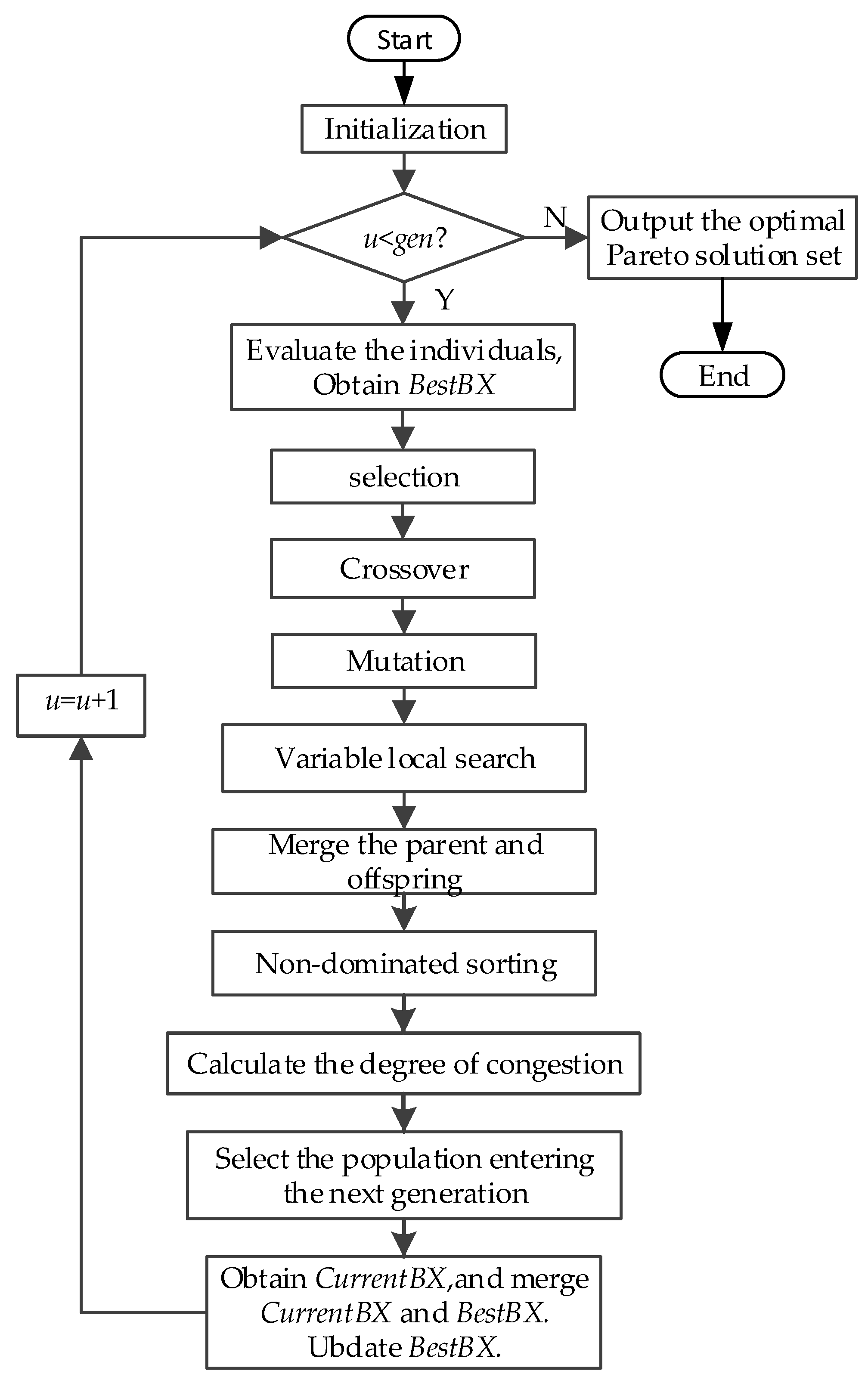
The genetic algorithm is an intelligent optimization algorithm based on natural evolution and selection, which has been widely used in many fields such as combinatorial optimization, machine learning, signal processing, adaptive control and artificial life. The genetic algorithm has the advantages of strong global search ability, fast speed and easy implementation, but it is easy to premature convergence. Combining local search with the genetic algorithm can improve the optimization ability of the genetic algorithm. A novel hybrid NSGA-II algorithm with variable local search is proposed, which integrates the advantages of a variable local search and NSGA-II. The variable local search is based on the various neighborhood structures.

4.1. The Flowchart Procedure of the HNSGA-II

The flowchart of the algorithm is shown in Figure 6.

4.2. The Details of the HNSGA-II

4.2.1. Encoding and the Population Initialization

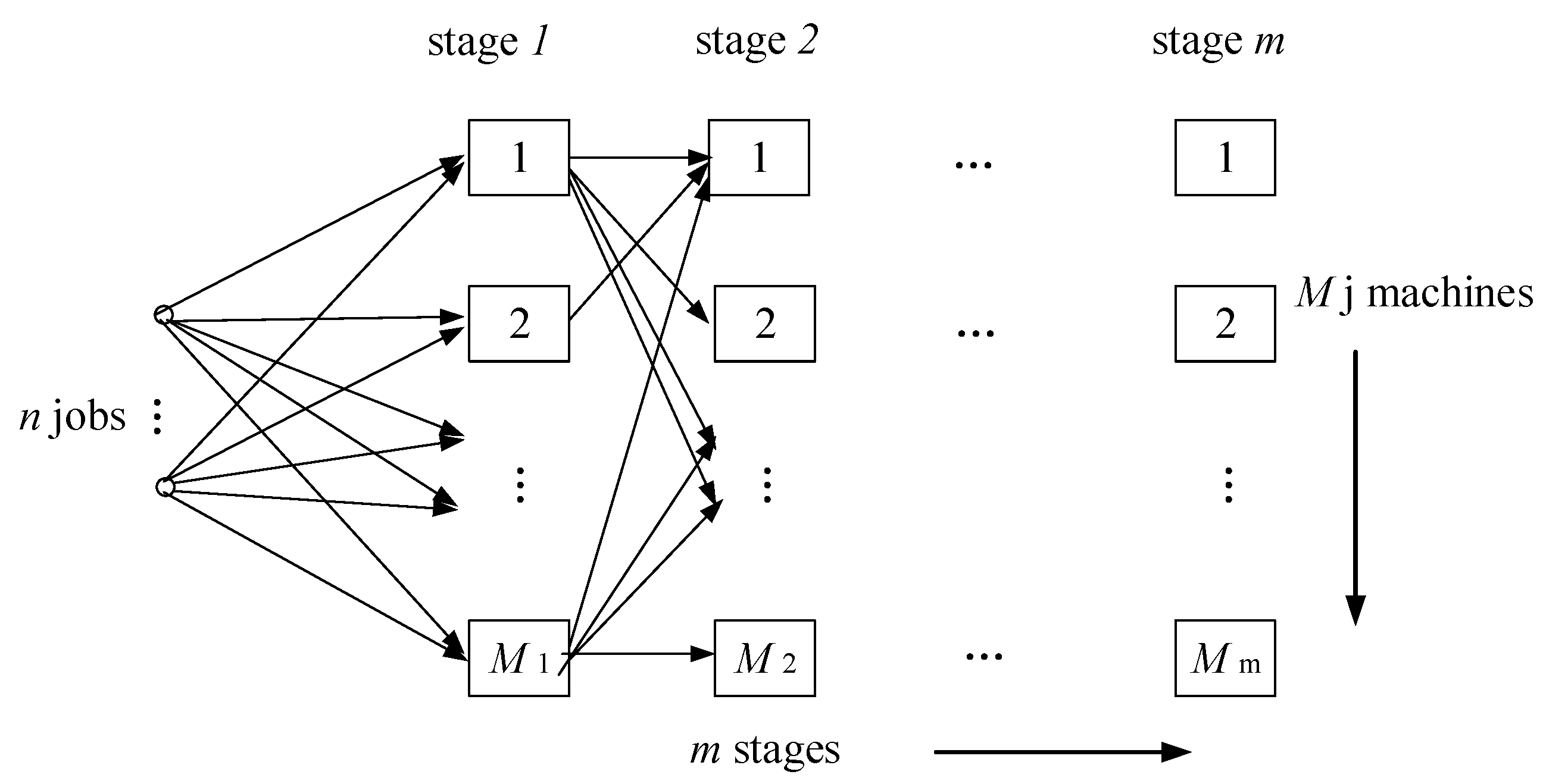
Due to the characters of the FFSP, the operation and machine based encoding method is employed. A chromosome consists of two parts: one is the processing order; the other is the machine assignment. Refer to the above instance of the turbine blades, $P_1$ is a chromosome.

$$P_1=\left[\begin{array}{c}24351\\ 21122\\ 34334\\ 55656\\ 78877\end{array}\right]$$

The number in the first row of the chromosome represents the jobs index. The position of the job number at the first row indicates the processing order of the job (2 4 3 5 1). The remainder of the chromosome is a $4\times 5$ matrix representing the assignment of machines at each stage. For example, $P_1\left(2,1\right)=2$ represents the job 2 is processed on machine 2 at stage 1, $P_1\left(3,1\right)=3$ represents the job 2 is processed on machine 3 at stage 2, $P_1\left(2,2\right)=1$ represents the job 4 is processed on machine 1 at stage 1. For each chromosome, the processing order of jobs is determined according to the position of each job that need to be processed, and the assignment of machines at each stage is determined on the basis of the remaining partial matrix.

If there is a problem with $n$ jobs, $m$ stages, a population of the HNSGA-II algorithm is initialized by randomly generating a group of $\left(m+1\right)\times n$ matrix as chromosomes. The scale of the population is $Psize$.

4.2.2. Low-Carbon Scheduling Decoding Algorithm

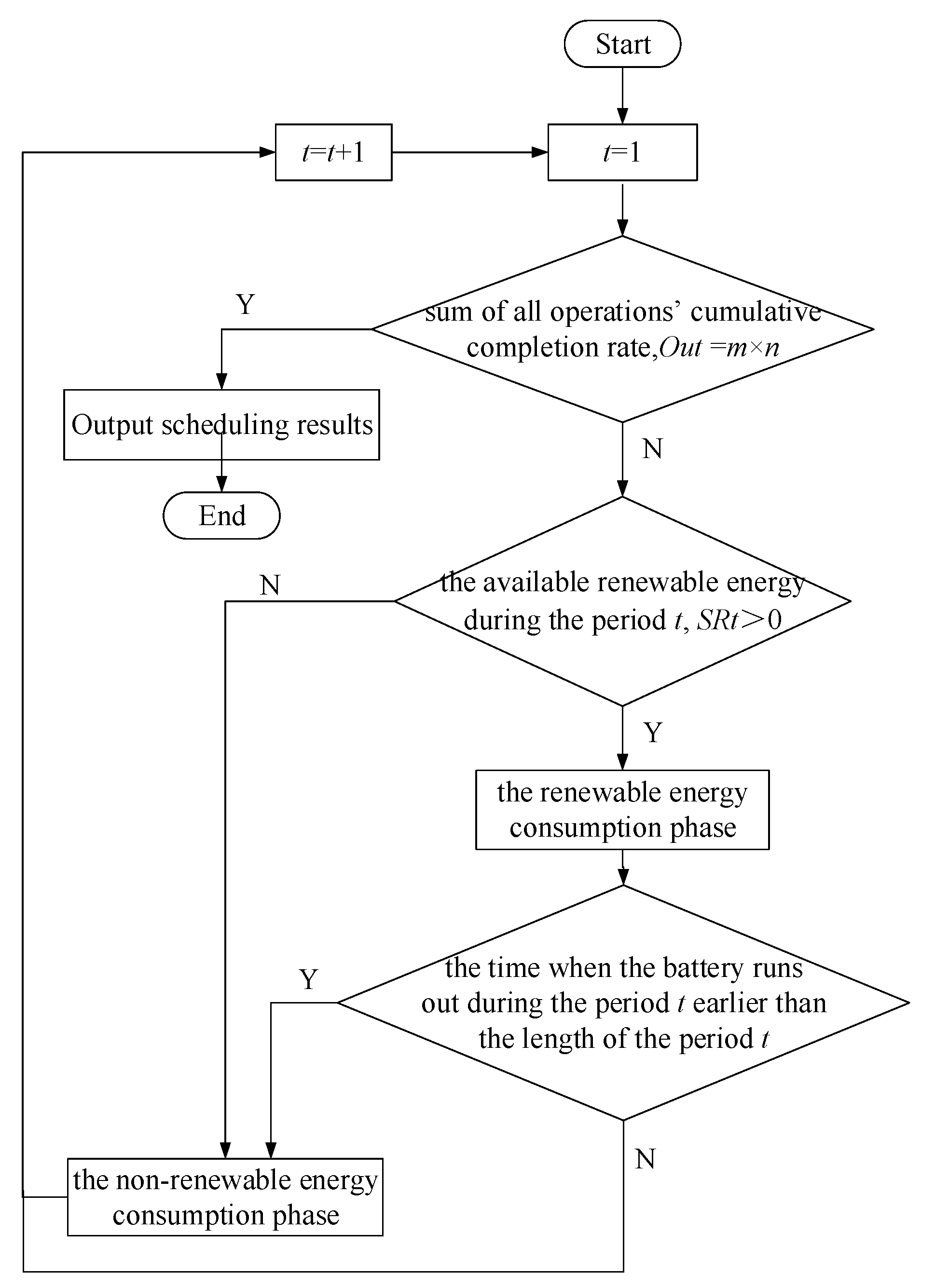
Taking into account the periodicity and randomness of power generated by solar energy, as well as the limited capacity of energy storage devices, solar energy cannot supply power to the workshop for a long time. Therefore, the production process is powered by solar energy and fossil fuel periodically. The power generation fluctuates randomly according to weather conditions and the available renewable power does not exceed the capacity of the energy storage device. Due to the features of solar energy, carbon dioxide will not be generated during the process of consuming the solar energy, whether in the process of production or in the idle time. Therefore, in order to ensure that enterprises can minimize their carbon footprint, they give priority to running the photovoltaic power station micro-grid for energy in isolation. When the energy in the energy storage device is exhausted, the micro-grid is switched to run in parallel, power is generated from the traditional power grid using the non-renewable energy, which generates carbon footprint.

Each period is divided into two parts: the renewable energy consumption phase and the non-renewable energy consumption phase. According to the processing order of jobs and the assignment of machines at each stage, the processing operations and the idle machines in each period can be determined. Based on the rule that prioritizes renewable energy, the following low-carbon scheduling algorithm can construct a low carbon scheduling solution. The flowchart of the low-carbon scheduling algorithm is shown in Figure 7. The detailed steps are as follows:

Step1: Set the number of period, $t=1$; the available renewable energy during period $t$, $S{R}_t=min\left(b_t,Q\right)$. Obtain the operation $O_{ij}$ which is processed at the beginning of the initial period based on the chromosome. Calculate the sum of the renewable energy consumption per unit time of the processing operations, $SumE$.

Step2: Calculate the sum of all operations’ cumulative completion rate, $Out$. If $Out=m\times n$, go to Step12; otherwise, go to Step3.

Step3: Calculate the time when the battery runs out during period $t$, that is, $Finishtime=S{R}_t/SumE$. Record the current renewable energy consumption of operations and the current completion rate of operations at the renewable energy consumption phase during period $t$.

Step4: Calculate the cumulative completion rate of the processing operations. If each cumulative completion rate of the processing operations is less than 1, let $S{R}_t=0$ and go to Step 8; otherwise, go to Step5.

Step5: Calculate the time when the first completed operation is finished processing at the renewable energy consumption phase, $Retime$. Recalculate the current renewable energy consumption and the current completion rate of operations at the renewable energy consumption phase from the beginning of period $t$ to $Retime$.

Step6: Determine whether all the completed operations have follow-up stage at $Retime$. If yes, then if the machine where the follow-up stage is processed does not start processing or is idle, the follow-up stage enters the processing state; otherwise, it will not be processed at $Retime$. Otherwise, go to Step7.

Step7: Determine whether all the machines on which the completed operations are processed have subsequent unprocessed operations that need to be processed at $Retime$ according to the chromosome. If all the subsequent unprocessed operations are not at the first stage and all the previous stages have not yet finished processing, processing will not be started and the machine keeps idle; If all the subsequent unprocessed operations are at the first stage or all the subsequent unprocessed operations are not at the first stage and any the previous stage is completed, the subsequent unprocessed operations are arranged to enter the processing state according to the following rules:

• The shortest renewable processing time of the subsequent unprocessed operations have first priority.
• If the renewable processing time is the same, the lowest renewable energy processing energy consumption per unit time of the subsequent unprocessed operations has second priority.
• If the energy consumption is the same, select one randomly.

The priority order of the subsequent unprocessed operations selected for the processing state is: the processing time $\succ$ processing energy consumption per unit time.

Step8: Update $S{R}_t$. Calculate $Out$, if $Out=m\times n$, go to Step12. Otherwise, if $S{R}_t>0$, proceed to Step3; otherwise, go to Step9.

Step9: If the time when the battery runs out during period $t$ earlier than the period length of period $t$, that is, $ReNewableTime<Length\left(t\right)$, then calculate the remaining time of period $t$, that is, $RonReTime=Length\left(t\right)-ReNewableTime$, go to Step10; otherwise, let $t=t+1$, go to Step3.

Step10: Refer to Step3-Step7, calculate the non-renewable energy consumption of operations and the completion rate of operations at the non-renewable energy consumption phase of period $t$. If any operation is completed during this time, select unprocessed operations into the processing state according to the priority order: the processing time $\succ$ processing energy consumption per unit time.

Step11: Update $NonReTime$. Calculate $Out$, if $Out=m\times n$, go to Step12. Otherwise, if $NonReTime=0$, let $t=t+1$, go to Step3; otherwise, go to Step10.

Step12: Calculate all operations’ starting time and completing time using the renewable energy and the non-renewable energy during each period respectively based on all operations’ renewable energy consumption and non-renewable energy consumption during each period. Output the scheduling solution and the energy scheduling assignment. Calculate the makespan according to the scheduling solution. Calculate the total carbon footprint.

4.2.3. Crossover

Crossover operator is the intersection of two parent chromosomes. It could obtain more excellent chromosomes through crossover. Among the various genetic algorithms for solving FFSP, most of the crossover operators use the position-based crossover (PBX) and the liner order crossover (LOX) [35]. Therefore, considering the coding characteristics of the chromosomes, the crossover operator integrating the LOX with PBX is proposed.

The flowchart of the algorithm for crossover is shown in Figure 8. The detailed steps are as follows:

Step1: Randomly generate an integer between 1 and 2. If it is 1, go to Step2; if it is 2, go to Step3.

Step2: LOX is performed on the first row of the two parent individual matrixes to obtain the first row of the two offspring individual matrixes, and go to Step4.

Step3: PBX is performed on the first row of the two parent individual matrixes to obtain the first row of the two offspring individual matrixes, and go to Step4.

Step4: Randomly generate a binary array of size $1\times m$.

Step5: For row 2 to row $m+1$ of the parent individual matrix, starting from the first column, from left to right, each column is sequentially evaluated from top to bottom according to the $1\times m$ binary array, if it’s 0, the gene of the parent 1 at this position is inherited to the offspring 1 and the gene of the parent 2 at this position is inherited to the offspring 2; If it is 1, the gene of the parent 1 at this position is inherited to the offspring 2 and the gene of the parent 2 at this position is inherited to the offspring 1.

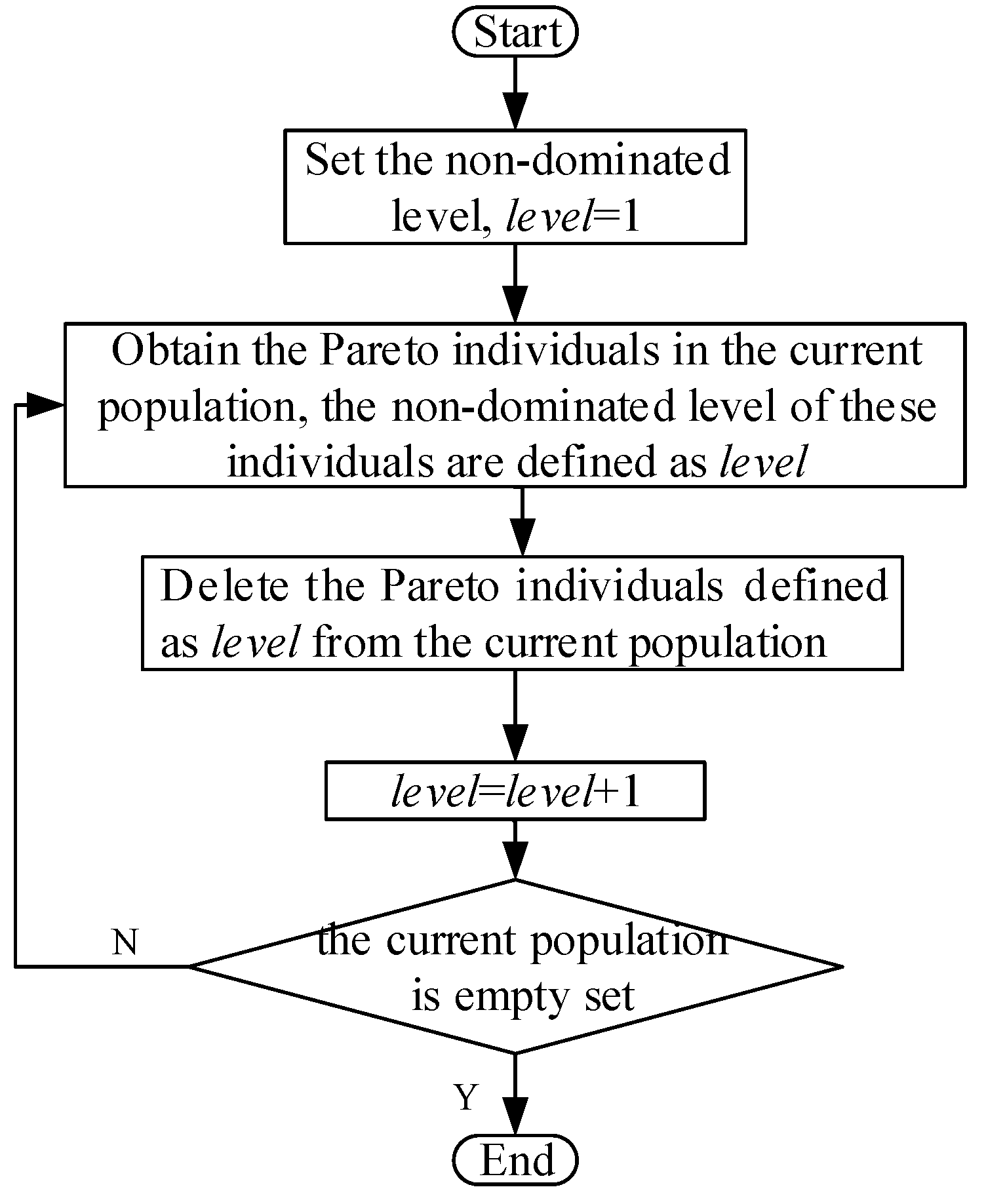
4.2.4. Non-Dominated Sorting Crossover

For the sorting of the non-dominated levels in the algorithm, the definition of Pareto non-dominated solution should first be defined. A non-dominated solution is the solution that is not dominated by any other feasible solution. The dominated relationship for a minimization is for any two feasible solutions $X_1$ and $X_2$, if the following conditions are satisfied,

$$\forall \ell ,f_{\ell }\left(X_1\right)\le f_{\ell }\left(X_2\right),\ell \in \{1,2,\dots ,r\},X_1,X_2\in Psize;$$

$$\exists \ell ,f_{\ell }\left(X_1\right)<f_{\ell }\left(X_2\right),\ell \in \{1,2,\dots ,r\},X_1,X_2\in Psize.$$

Then we call $X_1$ dominates $X_2$, shown as $X_1\succ X_2$, $X_1$ is the non-dominated solution, $X_2$ is the dominated solution [36], $r$ is the total number of the objectives.

If $X_1$ is not dominated by other individuals in the population, then $X_1$ is recorded as the Pareto non-dominated solution, that is, the Pareto optimal solution. The set of all the non-dominated solutions is the Pareto optimal solution set.

In order to select the best individual to enter the next generation, all the individuals in the population are divided into different non-dominated levels. The individuals in a lower level are selected preferentially to the next generation. The non-dominated ranking algorithm is proposed. The flowchart of the non-dominated ranking algorithm is shown in Figure 9.

4.2.5. The Crowding Degree Comparison Operator

After combining the parents and the offspring, calculate the crowding degree, which ensures the diversity of population and the population evolve toward a better direction. The definition of crowding degree is in Equation (20). The objective values of all individuals at the same non-dominated level are sorted in ascending order, and then calculate the average side length of the rectangle composed of $X_{i-1}$ and $X_{i+1}$, that is the crowding degree of $X_i$. The calculation procedure of the crowding degree is as follows:

Step1: Let ${Cr}_i=0,i=1,2,\dots num$, the crowding degree of $X_i$, $\mathrm{num}$ for the total number of individuals at the same non-dominated level.

Step2: Calculate the crowding degree of $X_i$:

$$C{r}_i=\frac{1}{2}{\displaystyle \sum }_{k=1}^2\frac{f_k\left(i+1\right)-f_k\left(i-1\right)}{f_k^{max}-f_k^{min}}$$

(20)

The crowding degree of the two boundary points: $C{r}_1=\infty$, $C{r}_{num}=\infty$. $X_{i-1}$, $X_i$ and $X_{i+1}$ are adjacent Pareto individuals at the same non-dominated level. $f_k^{max}$ denotes the maximum value of the k-th objective, $f_k^{min}$ denotes the minimum value of the k-th objective function. Two objectives are studied in this paper, so the value of $k$ is 1 and 2.

The crowding degree of $X_i$ is shown in Figure 10. It can be seen from Figure 10 that the smaller $C{r}_i$ is, the more crowded around $X_i$ is.

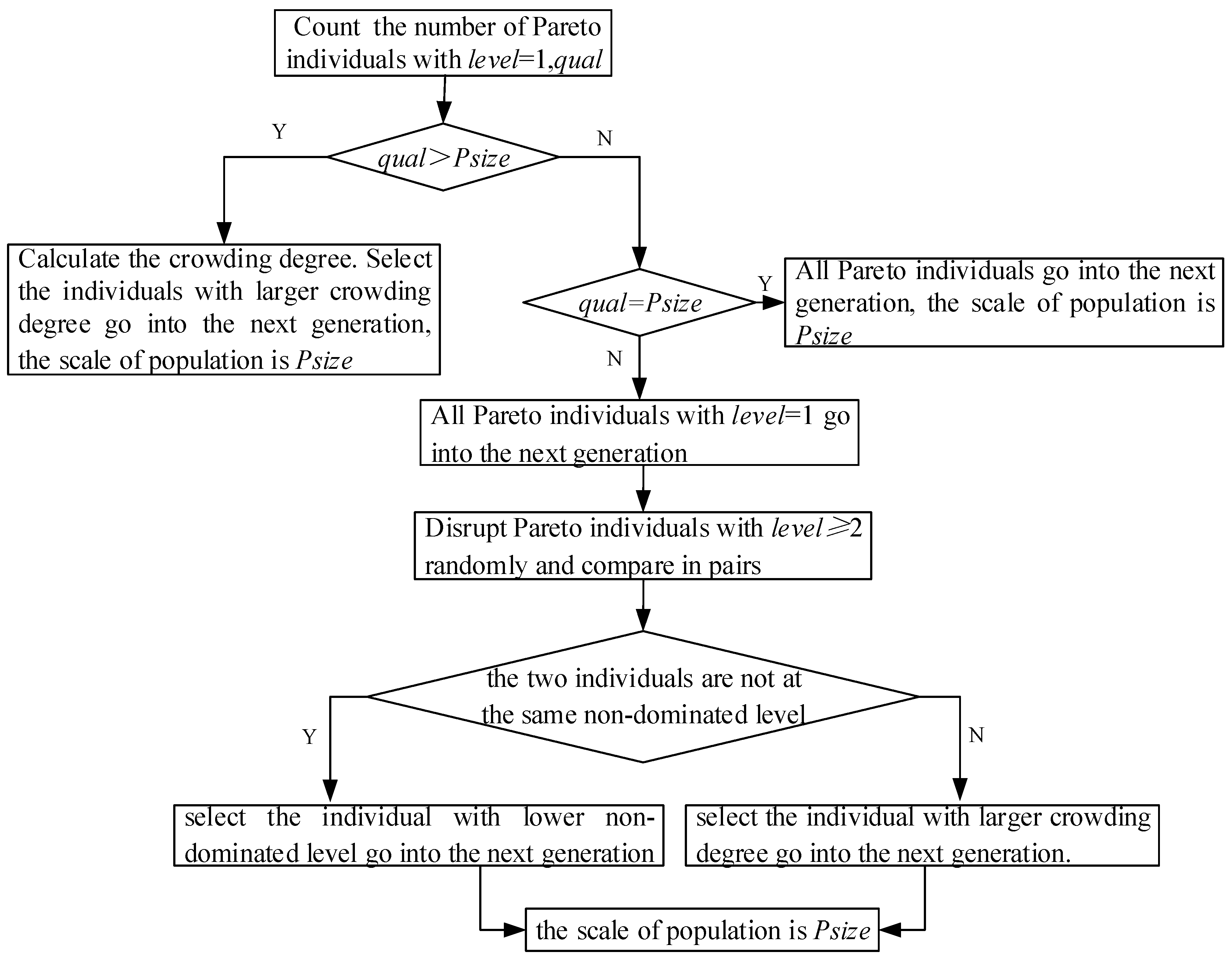
Individuals entering the next generation are selected based on the non-dominated level and the crowding degree. The flowchart of selecting individuals is shown in Figure 11. The detailed steps are as follows:

Step 1: Count $qual$, the number of Pareto individuals with $level=1$. If $qual>Psize$, go to Step2; if $qual=Psize$, go to Step3; if $qual<Psize$, go to Step4.

Step2: Calculate the crowding degree. Select the individuals with larger crowding degree go into the next generation, the scale of population is $Psize$.

Step3: All Pareto individuals go into the next generation, the scale of population is $Psize$.

Step4: All Pareto individuals with $level=1$ go into the next generation. Then, disrupt Pareto individuals with $level\ge 2$ randomly. Compare in pairs, if the two individuals are not at the same non-dominated level, select the individual with lower non-dominated level go into the next generation, otherwise, select the individual with larger crowding degree go into the next generation. The scale of population is $Psize$.

Chromosomes with a lower non-dominated level are selected into the next generation, which can keep the elite individuals in the population to a great extent. The diversity of the population can be ensured by selecting individuals with a larger crowding degree at the same non-dominated level.

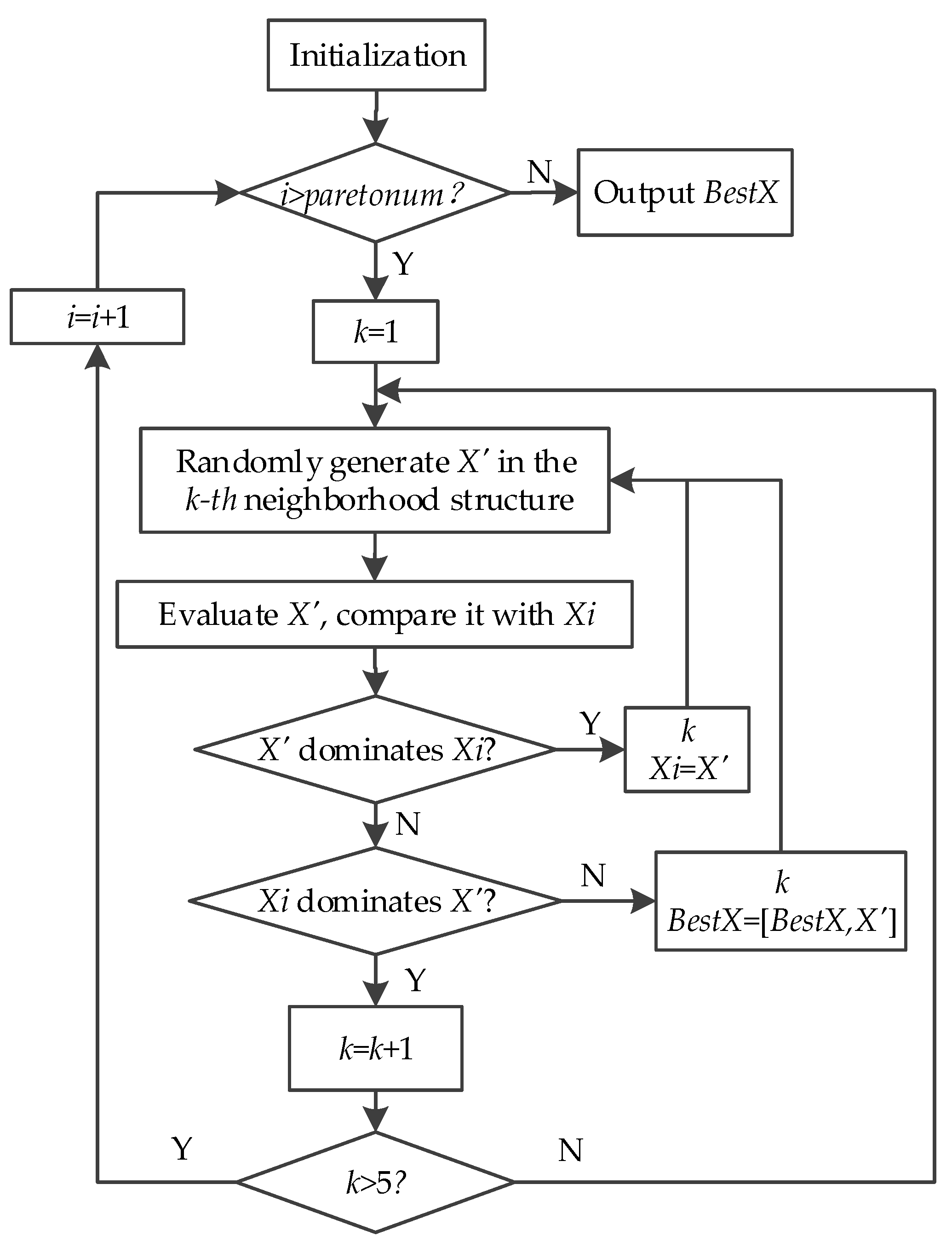
4.2.6. Variable Local Search Strategy

It is easy for the genetic algorithm to fall into a local optimum, so it is necessary to integrate a local search with the genetic algorithm. The primary problem in designing a variable local search strategy is to design the neighborhood structures. Considering the structure of FFSP, 5 kinds of local search methods are developed according to the operation and machine based encoding method. The traditional local search mainly includes swap and insert, which are relatively simple and easy to implement. Therefore, for the production scheduling problem, many algorithms use these two local search methods [37]. Besides, we develop another three local search methods: (1) reassign the machine of an operation, which is the mutation operation in this paper; (2) reassign the machines of all stages of a job, which is more complicated and has stronger local search ability than reassigning the machine of a operation; (3) Reverse the elements between two positions, which can produce a greater disturbance to the original chromosome, so that the algorithm cannot fall into the local optimum and expand the search space. Therefore, the 5 kinds of local search methods are as follows.

• Swap. Randomly select two positions in the first row of the chromosome, and then swap the whole column genes at the two selected positions.
• Insert. Randomly select two positions, $position1$ and $position2$, in the first row of the chromosome, where $position1<position2$. Then insert the whole column genes at $position2$ before those at $position1$.
• Reassign the machine of an operation. Randomly select one position in the machine assignment part of the chromosome, and then reassign the machine of the operation at the selected position.
• Reassign the machines of a job’s all stages. Randomly select one position in the first row of the chromosome, and then reassign all stages machines of a job at the selected position.
• Reverse the genes between two positions. Randomly select two positions in the first row of the chromosome, and then reverse the whole column genes between the two selected positions.

Based on the above 5 kinds of local search methods, the local search process is shown in Figure 12, specific steps are as follows:

Step1: Set $N_k,k=1,2,\dots ,5$. Input initialization parameters: the Pareto optimal solution set of the offspring, $BestX$; the i-th individual of $BestX$, ${\mathrm{X}}_{\mathrm{i}}$ Calculate the number of $BestX$, $paretonum$. Let $i=1$.

Step2: If $i>paretonum$, go to Step6; otherwise, let $k=1$.

Step3: Randomly generate a new solution $X^{\prime }$ according to the local search method $N_k$, $X^{\prime }$ is compared with $X_i$ by the crowding degree comparison operator.

Step4: If $X^{\prime }\succ X_i$ then $X_i=X^{\prime }$ and continue searching within the local search method $N_k$, go to Step3. If $X^{\prime }$ and $X_i$ are non-dominated by each other, then append $X^{\prime }$ to $BestX$ and continue searching within local search method $N_k$, go to Step3. If $X_i\succ X^{\prime }$, let $k=k+1$, go to Step5.

Step5: If $k>5$, then let $i=i+1$, go to Step2; otherwise, go to Step3, transfer to the next local search method.

Step6: Output $BestX$, calculate the number of the current $BestX$, $currentnum$. If $currentnum=paretonum$, then combine the parent and offspring directly; otherwise, from $i=paretonum+1$ to $i=\min \left(currentnum,Psize-paretonum\right)$, let $X_i$ replace the dominated solution in the offspring population in turn.

5. Numerical Experiments

5.1. Design of Experiment

All the experiments were conducted on a computer with Intel Core i5 2.7GHz CPU, 8 GB RAM, OS X EI Capitan, and Matlab. All of the parameters are set as:

• The population size, $Psize=100$;
• The iteration times, $gen=1000$;
• The crossover probability, $P_c=0.9$;
• The mutation probability, $P_m=0.2$.

Two groups of experiments are conducted:

(1)

The comparison of flexible flow shop scheduling with renewable energy (FFSP-RE) and flexible flow shop scheduling without renewable energy (FFSP). The aim is to verify the low-carbon scheduling algorithm can reduce the carbon footprint effectively under the premise of makespan optimization.

(2)

The evaluation of the HNSGA-II algorithm with a small-scale instance and a large-scale instance. The aim is to verify the performance of the HNSGA-II algorithm and compare our approach with NSGA-II.

The experiment data are based on the new energy industry and auto parts and high-end equipment manufacturing industries under the operation of a commercialized industrial area micro-grid project. Among them, the new energy industry selected wind turbine blade production, the experiment data are mentioned above in Section 3.1. We select the radial tire of Fengli Tire Company as a tire production case [38]. The process flow of radial tire production consists of mixing (two stages), preparing rubber, tire forming and vulcanization. Mixing needs to be divided into two separate sub-processes because two rubber mixing methods are adopted to mixing. Therefore, the process flow of the tire production can be seen as 5 stages. There are multiple parallel machines in each stage; the number of parallel machines at each stage is 4, 4, 2, 3 and 4 respectively. There are 10 tires that need to be processed. The processing time of each job on every machine in two types of power supply system is given in

Table A4. The processing time for the tire production instance.

Job No.	Stage 1										Stage 2
	M1				M2		M3		M4		M5		M6		M7		M8
	RE		NRE		RE	NRE	RE	NRE	RE	NRE	RE	NRE	RE	NRE	RE	NRE	RE	NRE
Job 1	44		22		40	20	48	24	53	26	64	32	58	29	70	35	77	38
Job 2	76		38		68	34	84	42	91	46	58	29	52	26	64	32	70	35
Job 3	60		30		54	27	66	33	72	36	74	37	67	33	81	41	89	44
ob 4	70		35		63	32	77	39	84	42	52	26	47	23	57	29	62	31
Job 5	56		28		50	25	62	31	67	34	78	39	70	35	86	43	94	47
Job 6	50		25		45	23	55	28	60	30	60	30	54	27	66	33	72	36
Job 7	66		33		59	30	73	36	79	40	48	24	43	22	53	26	58	29
Job 8	58		29		52	26	64	32	70	35	46	23	41	21	51	25	55	28
Job 9	74		37		67	33	81	41	89	44	62	31	56	28	68	34	74	37
Job 10	52		26		47	23	57	29	62	31	70	35	63	32	77	39	84	42
Job No.	Stage 3				Stage 4						Stage 5
	M9		M10		M11		M12		M13		M14		M15		M16		M17
	RE	NRE	RE	NRE	RE	NRE	RE	NRE	RE	NRE	RE	NRE	RE	NRE	RE	NRE	RE	NRE
Job 1	70	35	63	32	30	15	27	14	33	17	34	17	31	15	37	19	41	20
Job 2	54	27	49	24	54	27	49	24	59	30	50	25	45	23	55	28	60	30
Job 3	44	22	40	20	38	19	34	17	42	21	44	22	40	20	48	24	53	26
Job 4	64	32	58	29	56	28	50	25	62	31	38	19	34	17	42	21	46	23
Job 5	50	25	45	23	50	25	45	23	55	28	46	23	41	21	51	25	55	28
Job 6	66	33	59	30	34	17	31	15	37	19	42	21	38	19	46	23	50	25
Job 7	58	29	52	26	58	29	52	26	64	32	36	18	32	16	40	20	43	22
Job 8	72	36	65	32	36	18	32	16	40	20	48	24	43	22	53	26	58	29
Job 9	42	21	38	19	44	22	40	20	48	24	44	22	40	20	48	24	53	26
Job 10	60	30	54	27	52	26	47	23	57	29	50	25	45	23	55	28	60	30

(Appendix A). The energy consumption when jobs are processed on every machine in two types of power supply system is shown in

Table A5. The processing energy consumption for the tire production instance.

Job No.	Stage 1										Stage 2
	M1				M2		M3		M4		M5		M6		M7		M8
	RE		NRE		RE	NRE	RE	NRE	RE	NRE	RE	NRE	RE	NRE	RE	NRE	RE	NRE
Job 1	55		110		61	121	50	99	44	88	48	95	52	105	43	86	38	76
Job 2	44		88		48	97	40	79	35	70	50	100	55	110	45	90	40	80
Job 3	48		96		53	106	43	86	38	77	45	90	50	99	41	81	36	72
Job 4	46		92		51	101	41	83	37	74	52	104	57	114	47	94	42	83
Job 5	51		102		56	112	46	92	41	82	42	84	46	92	38	76	34	67
Job 6	53		105		58	116	47	95	42	84	49	97	53	107	44	87	39	78
Job 7	47		94		52	103	42	85	38	75	53	106	58	117	48	95	42	85
Job 8	50		100		55	110	45	90	40	80	54	107	59	118	48	96	43	86
Job 9	45		90		50	99	41	81	36	72	48	96	53	106	43	86	38	77
Job 10	52		104		57	114	47	94	42	83	46	92	51	101	41	83	37	74
Job No.	Stage 3				Stage 4						Stage 5
	M9		M10		M11		M12		M13		M14		M15		M16		M17
	RE	NRE	RE	NRE	RE	NRE	RE	NRE	RE	NRE	RE	NRE	RE	NRE	RE	NRE	RE	NRE
Job 1	23	46	25	51	24	48	26	53	22	43	105	210	116	231	95	189	84	168
Job 2	26	51	28	56	13	25	14	28	11	23	88	175	96	193	79	158	70	140
Job 3	28	55	30	61	18	36	20	40	16	32	92	183	101	201	82	165	73	146
Job 4	24	48	26	53	12	23	13	25	10	21	101	202	111	222	91	182	81	162
Job 5	27	53	29	58	15	29	16	32	13	26	90	180	99	198	81	162	72	144
Job 6	24	47	26	52	23	45	25	50	20	41	93	185	102	204	83	167	74	148
Job 7	25	50	28	55	11	21	12	23	9	19	103	206	113	227	93	185	82	165
Job 8	23	45	25	50	22	43	24	47	19	39	89	178	98	196	80	160	71	142
Job 9	29	57	31	63	16	32	18	35	14	29	92	183	101	201	82	165	73	146
Job10	25	49	27	54	19	38	21	42	17	34	88	175	96	193	79	158	70	140

(Appendix A). The energy consumption when machines are idle in two types of a power supply system is shown in

Table A6. The idle energy consumption for the tire production instance.

Machines	M1	M2	M3	M4	M5	M6	M7	M8	M9	M10	M11	M12	M13	M14	M15	M16	M18
RE	5	6	5	4	5	6	5	4	2	2	1	1	1	9	10	8	7
NRE	11	12	9	8	11	12	9	8	5	5	3	3	2	18	20	16	15

(Appendix A).

5.2. Results for the Comparison of FFSP-RE and FFSP

The aim of this experiment is to compare FFSP-RE and FFSP and to run the algorithms 30 times respectively. The experimental results are reported in

Table 2. Results for the comparison of FFSP-RE and FFSP.

Problems	Carbon Footprint	Makespan	Number of Pareto
FFSP-RE	8840.50	152	30
FFSP	16,978.96	117.6	8.27

.

It can be seen from Table 2 that in the 30 experiments, the average number of Pareto solutions obtained by FFSP-RE is 30, while the average number of Pareto solutions obtained by FFSP is 8.27. Compared with FFSP, FFSP generates a carbon footprint of 16,978.96 and it will reduce to 8840.50 by FFSP-RE. On average, about 38.49% of the carbon footprint is reduced.

As shown in Figure 13, the experimental results of FFSP-RE and FFSP are randomly extracted from the 30 experiments. The best carbon footprint convergence curves are shown in Figure 14 and Figure 15. Figure 16 presents the best makespan average convergence curves.

It can be seen from Figure 13, the number of Pareto solutions obtained by the FFSP-RE is 32, and the number of Pareto solutions obtained by is 9. It can be seen from Figure 14 and Figure 15, the initial best carbon footprint obtained by FFSP-RE is about half of that obtained by FFSP. It proves that FFSP-RE can effectively reduce the carbon footprint. Combined with Figure 13, when the makespan in Figure 13 is between 100 and 120 and the makspan of FFSP-RE and FFSP is close, the carbon footprint of FFSP-RE is lower 50% nearly than that of FFSP. It can be seen from Figure 16, the best makespan of FFSP-RE is significantly better than that of FFSP. Therefore, we can be confident in saying that FFSP-RE can reduce the carbon footprint effectively under the premise of makespan optimization, and has a larger optimization space and more alternative solutions.

5.3. The Evaluation of the HNSGA-II Algorithm

5.3.1. Results for the Wind Turbine Blade Production Instance

The purpose of this experiment is to test the performance of the HNSGA-II algorithm for solving the small-scale instance by comparing the experimental results of HNSGA-II and NSGA-II. In this experiment, the renewable energy generation period is 24h. The algorithms were run 15 times respectively. The experimental results are reported in

Table 3. Results for the wind turbine blade production instance.

Objectives	Average		Minimum		Maximum
	HNSGA-II	NSGA-II	HNSGA-II	NSGA-II	HNSGA-II	NSGA-II
Carbon footprint	435.99	451.54	151.66	151.66	989.88	962.54
Makespan	127.43	124.79	62.71	68.15	175.52	175.52
Number of Pareto	117	115	100	107	140	125

.

It can be seen from Table 3 that in the 15 experiments, the HNSGA-II algorithm outperforms the NSGA-II algorithm in both the objectives and the number of Pareto solutions. Figure 2 and Figure 3 in Section 3.1 show a scheduling Gantt chart and the corresponding energy scheduling Gantt chart for this instance. Figure 17 presents the best makespan average convergence curves with the HNSGA-II and the NSGA-II in the 15 experiments, and Figure 18 presents the comparison of the best carbon footprint average convergence curves between the HNSGA-II and the NSGA-II of 15 experiments for wind turbine blade production instance.

It can be seen from Figure 17 and Figure 18, the HNSGA-II algorithm combined with the variable local search is better than the NSGA-II algorithm in terms of convergence performance. Since the studied problem is an NP-hard problem, it is not easy to find the optimal solution within a limited time. The NSGA-II algorithm converges at around 300 generations, while the HNSGA-II algorithm has a better convergence performance than the NSGA-II algorithm. Because the instance of wind turbine blade production is a small-scale instance, it is easy to find the optimal solution for the carbon footprint, but the convergence rate of HNSGA-II is faster than that of NSGA-II.

For a more intuitive representation, the best makespan and the best carbon footprint of two algorithms obtained from the 15 experiments are sorted in ascending order, respectively. Figure 19 and Figure 20 show the comparison of the best makespan and the best carbon footprint for the wind turbine blade production example. It can be seen from Figure 19 and Figure 20, for wind turbine blade production instance, after sorting, two-thirds of the results of the HNSGA-II algorithm are better than the NSGA-II algorithm, and one-third of the results are the same as those of NSGA-II in term of the best makespan. For the objective of the carbon footprint, the results of the HNSGA-II algorithm are the same as those of the NSGA-II algorithm.

5.3.2. Results for the Tire Production Instance

The aim of this experiment is to test the performance of the HNSGA-II algorithm on a large-scale by comparing the experimental results of HNSGA-II and NSGA-II. In this experiment, the renewable energy generation period is 24 h. The algorithms were run 15 times respectively. The experimental results are reported in

Table 4. Results for the tire production instance.

Objectives	Average		Minimum		Maximum
	HNSGA-II	NSGA-II	HNSGA-II	NSGA-II	HNSGA-II	NSGA-II
Carbon footprint	8335.05	8420.14	6219.60	6433.14	11,012.34	10,983.52
Makespan	63.80	65.78	42.67	44.51	108.53	106.25
Number of Pareto	168	157	104	131	214	192

.

As shown in Table 4, in the 15 experiments, the HNSGA-II algorithm outperforms the NSGA-II algorithm in both objectives and the number of Pareto solutions. Figure 21 presents the comparison of the best makespan average convergence curves between HNSGA-II and NSGA-II in 15 experiments for tire production instance, and Figure 22 presents the comparison of the best carbon footprint average convergence curves between HNSGA-II and NSGA-II of 15 experiments for tire production instance.

It can be seen from Figure 21 and Figure 22 that the HNSGA-II algorithm combined with the variable local search outperforms the NSGA-II algorithm in convergence performance. As shown in Figure 21, the HNSGA-II algorithm is superior to the NSGA-II algorithm in convergence rate and convergence performance in the pre-iteration, and the convergence rate and convergence performance of the two algorithms are comparable in the mid-iteration. However, in the late iteration, HNSGA-II algorithm jumps out of the local optimal solution and finds a better solution. The optimization result is better than that of the NSGA-II algorithm. As shown in Figure 22, the HNSGA-II algorithm outperforms the NSGA-II algorithm in terms of the convergence rate and the convergence performance. Figure 23 shows that the comparison of the best Pareto solutions between HNSGA-II and NSGA-II for the tire production example.

It can be seen from Figure 23 that the HNSGA-II algorithm is far superior to the NSGA- II algorithm in term of the makespan and the carbon footprint, and the best Pareto solution set obtained by the HNSGA-II algorithm completely dominates that obtained by the NSGA-II algorithm. In summary, the HNSGA-II algorithm combined with the local search strategy performs well both on a small-scale and a large-scale, and outperforms the NSGA-II algorithm.

For a more intuitive representation, the best makespan and the best carbon footprint of two algorithms obtained from 15 experiments are sorted in ascending order respectively. Figure 24 and Figure 25 shows that the comparison of the best makespan and the best carbon footprint for the tire production example. It can be seen from Figure 24 and Figure 25, for the tire production case, after sorting, the results of the HNSGA-II algorithm are all better than those of the NSGA-II, whether in the best makespan or in the best carbon footprint.

Figure 26 shows the Gantt chart of a scheduling solution for the tire production instance. The numbers in each rectangle indicate (job number, stage number). Figure 27 shows a Gantt chart of the corresponding energy scheduling solution. The number in each rectangle indicates energy consumption. The green part means that the job is processed with the renewable energy power supply system during the green part time, while the red part means that the job is processed with the non-renewable energy power supply system during the red part time.

5.4. Discussion

In summary, FFSP-RE can reduce carbon footprint effectively under the premise of makespan optimization, has a larger optimization space and more alternative solutions. In term of FFSP, due to the fixed energy consumption of the job on each machine, the carbon footprint can be optimized only by giving preference to low energy consumption machines and reducing the idle time of machines, which result in less optimization space and fewer Pareto solutions. The idle energy consumption of the machine is lower than its processing energy consumption. Therefore, the carbon footprint result obtained by FFSP is not excellent. In terms of FFSP-RE, due to the periodicity of renewable energy, renewable energy will be generated at every period. When the makespan is across more periods, the amount of renewable energy consumed in production will increase, the carbon footprint will be reduced correspondingly, the space for optimization will be expanded, and the number of Pareto solutions will increase.

Besides, no matter the small-scale instance or the large-scale instance, the HNSGA-II algorithm combined with variable local search is superior to the NSGA-II algorithm in terms of convergence performance and the quality of the Pareto optimal solution set. On the one hand, GA has the advantage of strong global search ability, fast speed and easy implementation, but it is susceptible to premature convergence. Combining with local search, the genetic algorithm has stronger search ability and can jump out of the local optimal solution. On the other hand, 5 kinds of local search methods are developed. From the first neighborhood method to the fifth neighborhood method, the neighborhood space expands in turn. As shown in Figure 12, a neighborhood method with a small change is used to optimize the solution. When the neighborhood method with a small change cannot optimize the solution, a neighborhood method with a large change is used. In this way, the HNSGA-II algorithm can not only jump out of local optimization, but also speed up the convergence speed.

6. Conclusions

In this study, considering the periodicity and the limited storage capacity of renewable energy, a mathematical model for the MFFSP-VPTRE is formulated. The objectives of the model are the total carbon footprint and the makespan. The HNSGA-II algorithm combined with a variable local search is proposed to solve the MFFSP-VPTRE and the low-carbon scheduling algorithm is developed. Finally, by comparing FFSP-RE and FFSP, it is proven that FFSP-RE can effectively reduce the carbon footprint under the premise of makespan optimization and has a larger optimization space and more alternative solutions. Comparison of the experimental results of HNSGA-II and NSGA-II proved that the HNSGA-II algorithm can solve the MFFSP-VPTRE more effectively and efficiently than the NSGA-II algorithm.

In the future, it will be interesting to investigate the following issues:

• To improve the variable local search process;
• To explore more practical constraints such as the transportation time between adjacent stages.