Social Sustainability Assessment across Provinces in China: An Analysis of Combining Intermediate Approach with Data Envelopment Analysis (DEA) Window Analysis

Abstract

There are two categories (i.e., radial and non-radial category) in conventional DEA (Data Envelopment Analysis). Recently, intermediate approach was put forward as a new third category. Intermediate approach is a newly proposed approach and there are quite limited related studies. This study contributes to the DEA studies by putting forward an analytical framework of combining intermediate approach and DEA window analysis along with the concepts of natural and managerial disposability. Such combination is quite meaningful and this new approach has three important features. To the best of our knowledge, such type of research has never been investigated by the existing studies. As an application, this approach is used to evaluate the performance of provinces in China from 2007 to 2014. Furthermore, this study develops a series of performance indices from different perspectives. This study identifies the three important findings. Firstly, eco-technology advancements can achieve economic prosperity and environmental protection simultaneously, and thus should become a new direction of climate policies. Secondly, considerable differences exist in a series of indices that evaluates the performance of various provinces and pollutants from different respective. Then, sufficient attention should be given to the provinces and the pollutants with poor performance. Finally, the Chinese government should promote efficiency improvement by “catching up” for provinces with poor performance in the short term. In addition, the central government should reduce regional disparity in order to promote the social sustainability in the long term.

1. Introduction

China is the world’s largest energy consumer along with serious environmental issues, and hence the Chinese government should adopt effective policies to enhance the sustainability levels. At present, China is the largest primary energy consumer and the largest CO₂ emitter in the world. According to [1], China’s primary energy consumption was 3053 million tons of oil equivalent (Mtoe) in 2016, accounting for 23.0% of the world total. Historically, there were rapid increases in China’s energy consumption. China’s primary energy consumption in 2016 was 3.03 times of that in 2000 and 1.23 times of that in 2010. Following rapid increases in energy consumption along with coal-dominated energy consumption mix, China’s CO₂ emission grew rapidly, too. According to [2], China’s CO₂ emissions reached 9087 million tons in 2014, standing for 28.06% of the world’s total. In addition, China experienced large emissions discharges (emissions for short, hereafter) of other pollutants. According to [3], in 2014, China’s emissions reached 19.74 million tons for SO₂, 17.41 million tons for soot and dust, 22.95 million tons for COD, 2.39 million tons for Ammonia Nitrogen and 71.6 billion tons for waste water. Because of large emissions of various pollutants, China faces serious environmental issues. Under such background, the Chinese government should adopt effective policies to protect the environment and promote social sustainability.

It is important to tradeoff between environmental protection and economic growth. One important worry of implementing sustainability policies is that environmental policies will go at the expense of economic growth, such as [4,5,6,7]. Fortunately, this is not necessarily true. Traditional DEA (Data envelopment analysis) cannot evaluate environmental protection and economic growth in a unified framework. To overcome this issue, Sueyoshi and his associates (such as [8,9,10]) put forward the concepts of natural and managerial disposability, where pollution reduction and economic growth can be assessed simultaneously. Following [11,12], social sustainability in this study is defined as a unified indicator of the amounts of desirable outputs (reflecting the levels of economic growth) and undesirable outputs (showing the degrees of environmental protection).

Based on the previous studies, this study contributes to DEA studies in the following two aspects.

Methodologically, this study contributes to DEA studies by putting forward an analytical framework of combining intermediate approach and DEA window analysis along with the concepts of natural and managerial disposability. This new approach has three important features. (1) This approach incorporates intermediate approach and thus unified inefficiency scores are obtained by calculating the inefficiency scores of all production factors. (2) This approach incorporates DEA window analysis, thus allowing for shifts of frontiers across time periods. This incorporation is quite meaningful, since it can produce more steady results in time trends of performance indices. (3) This approach is based on the concepts of natural and managerial disposability and thus allows for simultaneous achievement of economic growth (in terms of desirable outputs) and environmental protection (in terms of undesirable outputs). In this way, this study measures the sustainability levels of provinces in China. To the best of our knowledge, such type of study has never been explored in the previous studies of China’s environmental assessment.

Meanwhile, this study makes empirical contributions by adopting the above new methodology to China’s provincial environmental assessment from 2007 to 2014. In this regard, this study develops a series of indices, which can capture dynamic changes of environmental efficiency across provinces in China. So, this study can provide detailed information regarding the differences in efficiency scores across provinces and pollutants and such information is important and valuable to the policy makers in China.

The rest of this paper is organized as follows: Section 2 reviews the related literature. Section 3 presents the background of the regional gaps and the current environmental policies in China. Section 4 describes the method and introduces the performance indices. Section 5 reports the data and analyzes the obtained results. Section 6 presents the conclusions.

2. Literature Review

This study adopts combines intermediate approach and DEA window analysis along with natural and managerial disposability. As an application, this method is used to China’s environmental assessment. Then, three lines of research are highly linked with this study.

The first line of study is related to the DEA studies, especially about the intermediate approach. DEA was initially put forward by [13]. The authors developed the first DEA model, which was known as CCR model (named according to the acronym of the authors). Thereafter, DEA has been widely used in measuring relative efficiency of different decision units (DMU) in various research field.

DEA has its own advantages and disadvantages. Up to now, DEA has gained good academic reputation, because of its appealing advantages (such as non-parametric and simplicity in computation). Meanwhile, DEA suffers from several shortcomings such as methodological bias, sensitivity to atypical observations [14,15,16]. During the development of DEA, many researchers made contributions such as [17,18,19,20,21,22,23,24,25,26]. Ref. [16,21] provided the literature surveys on recent studies about energy and environmental performance assessment.

Recently, the newly-proposed intermediate approach is a combination of radial and non-radial approaches, and has several unique features. Formally, intermediate approach was first put forward by [11]. The authors argued that there were several unique features of intermediate approach. [27] made a methodological comparison among these three approaches. To the best of our knowledge, there are only two existing papers about intermediate approaches up to now. In this respect, this study contributes to the DEA studies by putting forward an analytical framework of combining intermediate approach and DEA window analysis along with the concepts of natural and managerial disposability.

The second line of research is about the window analysis. By creating a moving average analogue, window analysis technique treats a DMU in different time periods as “different” DMU and compares its performance across time periods along with the performances of other DMUs [14]. In this way, window analysis can catch the dynamic changes in unified efficiency over time. This method was initially put forward by [28] and thereafter some other studies made significant contributions to this line of research, such as [14,29,30]. The advantages and disadvantages of window analysis was summarized by [31]. It is noteworty that this method creates new efficiency frontiers by combining some consecutive years into period blocks, thus allowing for shifts of frontiers between periods. Recent applications can be found in [9,32,33].

The third line of research is about environmental assessment in China. China has attracted great academic research interest, because it is a large developing country with serious environmental issues. This study concentrates on the DEA studies on China’s regional performance and

Table 1. The previous DEA studies about regional assessment of China.

Authors	Desirable Outputs	Undesirable Outputs	Production Inputs
[34]	GDP	SO2, COD, Nitrogen	Labor, capital, energy, water
[35]	GDP	CO2	Labor, capital, energy
[36]	GDP	CO2, SO2	Labor, capital, coal, crude oil, natural gas
[37]	Industrial added value	CO2	Labor, capital, energy
[38]	GDP		Labor, capital, energy
[39]	GDP	Waste water, waste gas, solid waste	Labor, capital, energy
[40]	Industrial added value	CO2, SO2	Labor, capital, energy
[41]	Industrial added value	NO2	Capital, electricity
[26]	GDP	CO2	Labor, capital, energy
[42]	GDP	CO2, SO2	Labor, capital, coal, electricity
[4]	GDP	CO2	Labor, capital, energy
[43]	GDP	CO2	Labor, capital, energy
[44]	GDP	Solid waste	Labor, capital, coal
[45]	GDP, primary secondary and tertiary industry	PM10, SO2, NO2	Coal, oil, gas, electricity, energy investment
[46]	Industrial added value	Waste water, solid waste	Labor, capital, coal
[22]	Industrial added value	CO2	Labor, capital, energy
[47]	GDP	SO2, solid waste	Labor, capital, energy
[48]	GDP	CO2, SO2, COD	Labor, capital, energy
[49]	GDP	CO2, SO2, solid waste, industrial dust	Labor, capital, energy
[50]	GDP	CO2	Labor, capital, energy
[6]	GDP	CO2	Labor, capital, energy
[51]	GDP	CO2, SO2	Labor, capital, energy
[52]	GDP	SO2, waste water, solid waste	Labor, capital, energy
[53]	GDP		Coal, oil, gas, fixed investment

lists the recent 24 studies from 2010 to 2017. From this table, one can see three interesting concerns. First, twenty-one studies are about environmental assessment and all studies incorporate energy performance. Hence, energy efficiency and environmental assessment become important research focuses. Second, there are fourteen studies about CO₂, ten studies about SO₂, six studies about solid waste and limited studies about other industrial pollutants. Thus, among all pollutants, CO₂ and SO₂ become important research focuses. Third, among twenty-one studies about environmental assessment, ten studies assess the performance of one pollutant, six studies assess the performance of two pollutants, five studies of three pollutants and one study assesses the performance of four pollutants.

Position of this research: This study clearly acknowledges the contributions of the existing research on DEA and the environmental assessment of China. An intermediate approach is a newly-proposed method and there have been quite limited related studies. [11] formally put forward this approach and [27] compared radial, non-radial and intermediate approaches. Based on the existing studies, this study contributes to the DEA studies by putting forward an analytical framework of combining intermediate approach and window analysis technique along with the concepts of natural and managerial disposability. This methodological extension is quite meaningful and this extended methodology has three important features, as detailed summarized in the end of Section 1. Therefore, it can be envisioned that this extended approach will produce empirical results with additional new information on China’s environmental evaluation. To the best of our knowledge, such kind of research has been never investigated by the previous studies.

3. China’s Regional Gaps and Current Environmental Policies

This section introduces the background of the research. Section 3.1 compares two major economic and energy indicators across provinces in China. The purpose is to introduce China’s regional gaps across provinces. Section 3.2 introduces China’s political organs about environmental protection and current environmental policies.

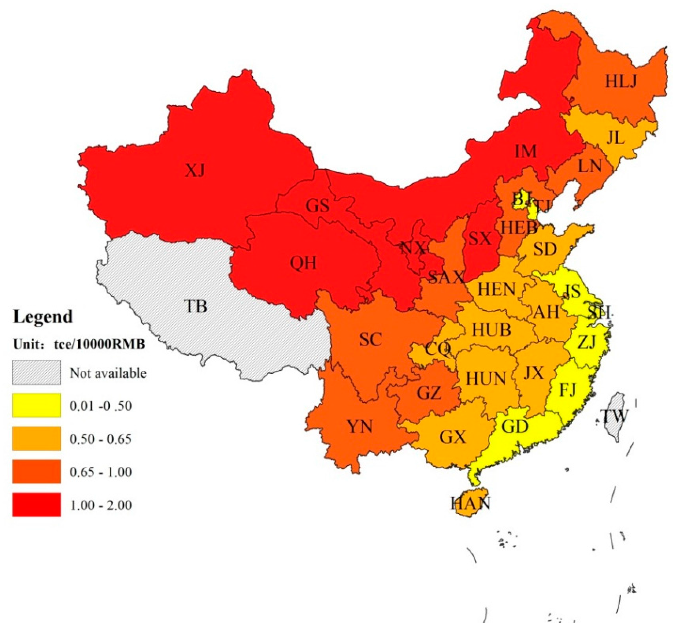
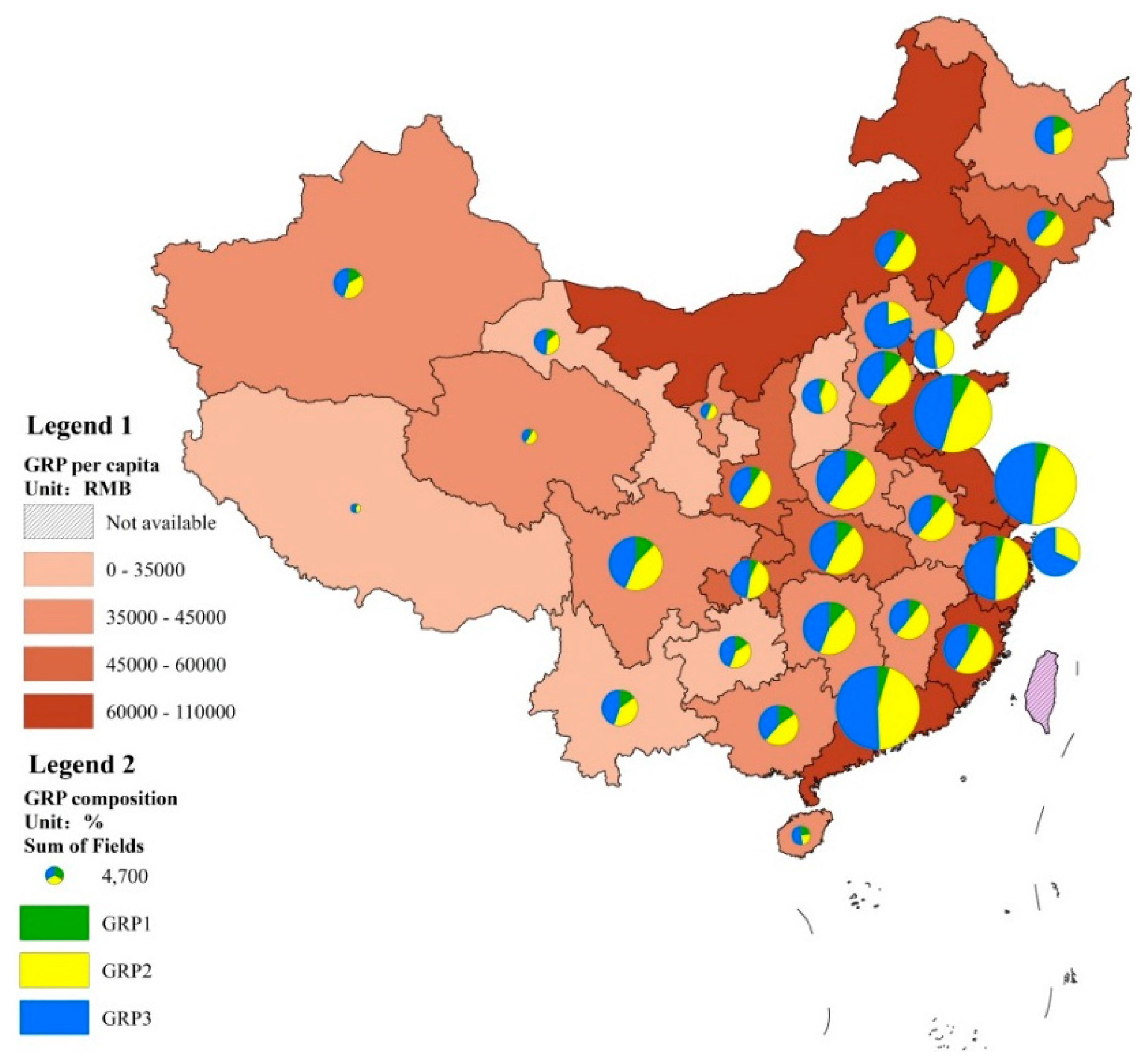
3.1. China’s Regional Disparity

China is a large developing country, with transitional economy and considerable regional gaps. To express regional disparity, this study considers two indicators (i.e., energy intensity and structure of economy) as examples.

Figure 1 demonstrates energy intensity across provinces in 2015, where energy intensity is calculated as energy consumption per unit of GRP (gross regional product). Figure 1 provides us two interesting concerns. Firstly, energy intensity of southern provinces is generally less than that of northern provinces. The main reason is that it is cold in winter in northern provinces and it consumes a large amount of coal for heating. By comparison, it is relatively warm in southern provinces and there are no heating systems at the city-level in south China, where the southern provinces and northern provinces are traditionally bordered by Qinling Mountains and the Huaihe River. Secondly, energy intensity in east coastal provinces is roughly less than that in central or western provinces. The main reason is that economy grows rapidly in eastern provinces because of geographical locations and favorable policies, as compared with other provinces. Most east coastal provinces belong to well-developed provinces and such provinces are usually associated with high-energy efficiency per unit of GRP.

Figure 2 illustrates GRP per capita and the structure of economy across provinces in China in 2015. Figure 2 provides us two interesting concerns. Firstly, GRP per capita in east coastal provinces are generally higher than that in central (or western) inland provinces. Thus, there are considerable differences in economic development levels among provinces. Secondly, there exist considerable differences in the structure of economy among provinces. In China, well-developed provinces are at the end of industrialization and thus tertiary industry accounts for a relatively large share in the economy. Under-developed provinces are still in the process of industrialization and urbanization and secondary industry accounts for a large share in the economy. In this case, well-developed provinces mainly concentrate on east coastal provinces and under-developed provinces are mostly inland provinces.

3.2. China’s Current Environmental Policies

This subsection provides a brief introduction to China’s environmental policies, where the information is obtained via websites of SC (The State Council of China) or MEP (The Ministry of Environmental Protection of China) without other clear statements.

Among all political organs, NPC (The National People’s Congress of China) is the highest organ. It has the right of enacting the laws, creating and supervising all the other political organs. During the past few years, NPC (or its Standing Committee) passed a series of laws about environmental protection. The laws involve air pollution, cleaner production, energy consumption, water pollution, solid waste, environmental protection and environmental impact.

SC is the central government and functions as an executive organ to implement administrative measures, rules and regulations. China is administratively divided into five tiers (i.e., provinces, cities, counties and towns, or their equivalents). There is a relatively rigid hierarchy among the governments, since the local governments follow the leadership of the central government and their respective upper-level governments.

The central government has set the targets of environmental protection with several policies to be implemented. The targets include Ammonia Nitrogen (to be reduced by 10%), COD (to be reduced by 10%), SO₂ (to be reduced by 15%) and nitrogen oxides (to be reduced by 15%) during the 13th Five-Year Plan period (2016–2020). The targets have been assigned to local governments, industries and enterprises. To achieve the targets, China develops the pollution rights trading systems and issues a series of standards. China plans to establish national pollution rights trading markets by 2020, with the purpose of promoting environmental industries and reducing environmental pollution effectively.

MEP is a branch of SC and functions as implementing environmental policies, laws and regulations. In 2016, MEP established many Central Environmental Inspection Teams. These teams follow the leadership of MEP and the central government and have the right to supervise environmental issues in the local governments. One important purpose of establishing such teams is to supervise the local governments to enhance environmental protection. Since then, they have established reputation of strictly implementing environmental protection.

4. Methodology

This study combines intermediate approach and DEA window analysis along with the concepts of natural and managerial disposability, after referring to the models in [10,11,27,56]. For the convenience of readers’ readability, this study reports the framework of the model.

4.1. The Production Technology Set and the Disposability Concepts

In this study, there are N DMUs. For every DMU, the production technology (T) transforms production inputs (x) into desirable outputs (y) and undesirable outputs (b). Technically, the production technology set (T) can be expressed in the following way:

$$T=\left\{\right(x,y,b):x \mathrm{can} \mathrm{produce} y \mathrm{and} b\}$$

(1)

In this study, many standard axioms of production theory are assumed to hold, such as the assumptions of bounded convexity and bounded set. See [19] for detail.

This study adopts the concepts of natural and managerial disposability. In this regard, there are two groups of disposability concepts (i.e., weak and strong disposability & natural and managerial disposability). The first group of concepts (weak and strong disposability) were initially put forward by [57], and now these concepts has been dominant in the existing studies. The second group of concepts was put forward by Sueyoshi and his associates, such as [8,9,11,12,27,45,56,58,59,60,61,62,63,64]. It is noteworthy that these two groups of disposability concepts do not conflict with each other, since weak disposability can become a special case of natural disposability. By comparison, managerial disposability can allow for a possible occurrence of desirable congestion, but weak and strong disposability (or natural disposability) cannot.

To incorporate the concepts of natural and managerial disposability, the production and pollution possibility sets exhibiting constant returns to scale ($P_c^{}$) can be written as follows:

$$P_c^N\left(x\right)=\left\{\begin{array}{c}\left(y,b\right):y\le {\displaystyle \sum _{n=1}^N{y}_n{\lambda }_n,b\ge {\displaystyle \sum _{n=1}^N{b}_n{\lambda }_n},x\ge {\displaystyle \sum _{n=1}^N{x}_n{\lambda }_n}}\\ {\lambda }_n\ge 0,n=1,\dots ,N\end{array}\right\}$$

(2)

$$P_c^M\left(x\right)=\left\{\begin{array}{c}\left(y,b\right):y\le {\displaystyle \sum _{n=1}^N{y}_n{\lambda }_n,b\ge {\displaystyle \sum _{n=1}^N{b}_n{\lambda }_n},x\le {\displaystyle \sum _{n=1}^N{x}_n{\lambda }_n}}\\ {\lambda }_n\ge 0,n=1,\dots ,N\end{array}\right\}$$

(3)

where c stands for the case of constant returns to scale. By contrast, the case of variable returns to scale can be derived easily, by adding the constraint (${\displaystyle \sum _{n=1}^N{\lambda }_n}=1$) into the above two axiomatic expressions. In this respective, the purpose of this study is to provide a combined approach and its empirical application to China’s environmental assessment. For simplicity, this study just considers the case of constant returns to scale.

The concepts of natural and managerial disposability rely on the constraints of production variables. The difference between natural and managerial disposability relies on the constraints of production inputs. The underlying meaning is that efficiency frontiers can be obtained by reducing production inputs for inefficient DMUs in the case of natural disposability, and by increasing production inputs in the case of natural disposability. The similarity between natural and managerial disposability relies on the constraints of desirable outputs and undesirable outputs. The underlying meaning is that efficiency frontiers can be achieved by increasing desirable outputs and/or undesirable outputs. Readers can turn to [16,56,60] for a detailed discussion. In such a setting, there can be simultaneous achievement of economic growth (in terms of desirable outputs) and environmental protection (in terms of undesirable outputs).

Meanwhile, this study restructures the data range following [11,45,61,62,64], which can be written as follows.

$$\begin{array}{l}{R}_m^x={\left(m+s+j\right)}^{-1}{\left[\max \left(\left|{\overline{x}}_{mnt}\right|\right)-\min \left(\left|{\overline{x}}_{mnt}\right|\right)\right]}^{-1}\\ R_s^y={\left(m+s+j\right)}^{-1}{\left[\max \left(\left|{\overline{y}}_{snt}\right|\right)-\min \left(\left|{\overline{y}}_{snt}\right|\right)\right]}^{-1}\\ R_j^b={\left(m+s+j\right)}^{-1}{\left[\max \left(\left|{\overline{b}}_{jnt}\right|\right)-\min \left(\left|{\overline{b}}_{jnt}\right|\right)\right]}^{-1}\\ n=1,\dots N;t=1,\dots ,T;m=1,\dots ,M;s=1,\dots ,S;j=1,\dots ,J.\end{array}$$

(4)

where R stands for a normalized weight vector of the production inputs and outputs.

4.2. Intermediate Approach and Unified Efficiency

The intermediate model under natural disposability can be specified as follows:

$$\begin{gathered} Maximize \frac{1}{S+J}\left({\displaystyle \sum _{s=1}^S{\xi }_s^y}+{\displaystyle \sum _{j=1}^J{\xi }_j^b}\right)+{\epsilon }_a\left({\displaystyle \sum _{m=1}^M{R}_m^x{d}_m^{x-}}+{\displaystyle \sum _{s=1}^S{R}_s^y{d}_s^y}+{\displaystyle \sum _{j=1}^J{R}_j^b{d}_j^b}\right) \\ \begin{array}{cccc}s.t.& {\displaystyle \sum _{n=1}^N{x}_{mn}{\lambda }_n}+d_m^{x-}\hfill & =& x_{ik},\hfill \\ & {\displaystyle \sum _{n=1}^N{y}_{sn}{\lambda }_n}-d_s^y-{\xi }_s^g{y}_{sk}\hfill & =& y_{sk},\hfill \\ & \hfill {\xi }_s^y& \le & 1,\\ & {\displaystyle \sum _{n=1}^N{b}_{jn}{\lambda }_n}+d_j^b+{\xi }_j^b{b}_{jk}\hfill & =& b_{jk},\hfill \\ & \hfill {\xi }_f^b& \le & 1,\\ & \hfill {\xi }_s^y\ge 0\left(r=1,\dots ,s\right),{\xi }_j^b& \ge & 0,\hfill \\ & \hfill {\lambda }_n\ge 0\left(n=1,\dots ,N\right),d_m^{x-}& \ge & 0,\hfill \\ & \hfill d_s^y\ge 0\left(r=1,\dots ,s\right), d_f^b& \ge & 0,\hfill \end{array} \\ m=1,\dots ,M;s=1,\dots ,S;j=1,\dots ,J. \end{gathered}$$

(5)

where ${\epsilon }_a$ is a very small positive number to decrease the influence of slack variables on the unified efficiency. β stands for a vector of scaling factors. ${\xi }_s^g$ stands for the inefficiency scores of desirable outputs. ${\xi }_j^b$ stands for the inefficiency score of undesirable outputs. d stands for slack variables.

The intermediate model equipped with managerial disposability can be specified as follows:

$$\begin{gathered} Maximize \frac{1}{S+J}\left({\displaystyle \sum _{s=1}^S{\xi }_s^y}+{\displaystyle \sum _{j=1}^J{\xi }_j^b}\right)+{\epsilon }_a\left({\displaystyle \sum _{m=1}^M{R}_m^x{d}_m^{x-}}+{\displaystyle \sum _{s=1}^S{R}_s^y{d}_s^y}+{\displaystyle \sum _{j=1}^J{R}_j^b{d}_j^b}\right) \\ \begin{array}{cccc}s.t.& {\displaystyle \sum _{n=1}^N{x}_{mn}{\lambda }_n}+d_m^{x-}\hfill & =& x_{ik},\hfill \\ & {\displaystyle \sum _{n=1}^N{y}_{sn}{\lambda }_n}-d_s^g-{\xi }_s^g{y}_{sk}\hfill & =& y_{sk},\hfill \\ & \hfill {\xi }_s^y& \le & 1,\\ & {\displaystyle \sum _{n=1}^N{b}_{jn}{\lambda }_n}+d_j^b+{\xi }_j^b{b}_{jk}\hfill & =& b_{jk},\hfill \\ & \hfill {\xi }_f^b& \le & 1,\end{array} \\ {\xi }_s^y\ge 0,{\xi }_j^b\ge 0,{\lambda }_n\ge 0, d_m^{x-}\ge 0,d_s^y\ge 0,d_f^b\ge 0, \\ n=1,\dots ,N;m=1,\dots ,M;s=1,\dots ,S;j=1,\dots ,J. \end{gathered}$$

(6)

In Models (5) and (6), the level of unified efficiency is divided into two subcomponents, where one subcomponents are related to desirable outputs and the other subcomponents are linked with undesirable outputs. One can obtain the average of the sum of these inefficiency subcomponents by solving Models (5) and (6).

4.3. Window Analysis

This study adopts the method in [10] to perform DEA window analysis. To incorporate the feature of “translation invariance”, this study begins with specifying the input and output variable within the time horizon.

$$\begin{array}{l}{\overline{x}}_{mn}=x_{mn}+{\alpha }_m,\\ {\overline{y}}_{sn}=y_{sn}+{\beta }_s,\\ {\overline{b}}_{jn}=b_{jn}+{\delta }_j,\\ n=1,\dots N;m=1,\dots ,M;s=1,\dots ,S;j=1,\dots ,J.\end{array}$$

(7)

Then, this study treats the observations for three consecutive years as a window and in this way new efficiency frontiers are created.

$$P_{PB\left(t\right)}=P_{t-2\cup t-1\cup t},\mathrm{for} t=3,\dots ,T$$

(8)

where PB stands for period block.

Finally, this study calculates the performance indices after solving Models (5) and (6).

4.4. Performance Indices of Inputs and Outputs

After referring to [11,19,20,21,65], this study defines two groups of performance indices.

The first group of performance indices include two indicators (i.e., UEI and BPI). This study begins with unified efficiency index (UEI). Suppose the variables with stars (e.g., ${\xi }^{\ast }s$ and $d^{\ast }s$) are the optional solutions to the DEA model. UEI is defined as the total unified efficiency (unity minus unified inefficiency). Technically, UEI is calculated as follows:

$$UEI=1-\left[\frac{1}{S+J}\left({\displaystyle \sum _{s=1}^S{\xi }_s^y{}^{\ast }}+{\displaystyle \sum _{j=1}^J{\xi }_j^b{}^{\ast }}\right)+{\epsilon }_a\left({\displaystyle \sum _{m=1}^M{R}_m^x{d}_m^{x-}{}^{\ast }}+{\displaystyle \sum _{s=1}^S{R}_s^y{d}_s^y{}^{\ast }}+{\displaystyle \sum _{f=1}^h{R}_j^b{d}_j^b{}^{\ast }}\right)\right]$$

(9)

where UEI stands for unified efficiency scores. Meanwhile, UEIM stands for unified efficiency scores under managerial disposability. UEIN stands for unified efficiency scores under natural disposability.

Then, this study considers the overall performance of undesirable outputs. To this end, this study develops an index performance index of aggregate pollutants, which is calculated as the potential efficiency of aggregate undesirable outputs divided by the potential efficiency of desirable outputs. Then, BPI is a measure of province-specific measure, and can be used to make comparisons in the overall performance of aggregate pollutants across provinces. Formally, BPI can be computed as follows:

$$BPI=\frac{Y/\left(Y+\frac{1}{S}{\displaystyle \sum _{s=1}^S{\xi }_s^y{}^{\ast }Y}+{\epsilon }_a{\displaystyle \sum _{s=1}^S{R}_s^y{d}_s^y{}^{\ast }}Y\right)}{B/\left(B-\frac{1}{J}{\displaystyle \sum _{j=1}^J{\xi }_j^b{}^{\ast }}B-{\epsilon }_a{\displaystyle \sum _{f=1}^h{R}_j^b{d}_j^b{}^{\ast }B}\right)}=\frac{1-\frac{1}{J}{\displaystyle \sum _{j=1}^J{\xi }_j^b{}^{\ast }}-{\epsilon }_a{\displaystyle \sum _{f=1}^h{R}_j^b{d}_j^b{}^{\ast }}}{1+\frac{1}{S}{\displaystyle \sum _{s=1}^S{\xi }_s^y{}^{\ast }}+{\epsilon }_a{\displaystyle \sum _{s=1}^S{R}_s^y{d}_s^y{}^{\ast }}}$$

(10)

where BPI stands for the performance index of aggregate undesirable outputs. Meanwhile, BPIM stands for BPI values under managerial disposability. BPIN stands for BPI values under natural disposability.

The above indicators (UEI and BPI) are bounded by zero and unity, where large values imply high unified efficiency. If the value is equal to unity, then the decision unit is fully efficient. If the value is less than unity, then the decision unit is inefficient.

The second group of performance indices include two indicators (i.e., RII and RETI). These indicators can be used to compare the efficiency of one pollutant relative to other pollutants. Their main differences rely on the scope of comparison. For one given province, RII is calculated as the relative efficiency of one pollutant divided by the overall efficiency of aggregate pollutants. Hence, RII is pollutant-specific efficiency measure relative to aggregate pollutants, which can be used to compare the relative efficiency of various pollutants in one given province. Technically, this index is calculated as follows:

$$RI{I}_j=\frac{1-\frac{1}{J}{\displaystyle \sum _{j=1}^J{\xi }_j^b{}^{\ast }}-{\epsilon }_a{\displaystyle \sum _{f=1}^h{R}_j^b{d}_j^b{}^{\ast }}}{\frac{1}{J}{\displaystyle \sum _{j=1}^J(1-\frac{1}{J}{\displaystyle \sum _{j=1}^J{\xi }_j^b{}^{\ast }}-{\epsilon }_a{\displaystyle \sum _{f=1}^h{R}_j^b{d}_j^b{}^{\ast }})}} (j=1,2,\dots ,J)$$

(11)

Meanwhile, RIIM stands for RII values under managerial disposability and RIIN stands for RII values under natural disposability.

RETI is calculated as the ratio of the efficiency of one pollutant in a time period and one province to the average efficiency of all pollutants in all time periods and all provinces. Then, RETI is also a pollutant-specific measure, which can be used to make comparisons across pollutants and provinces. Technically, RETI is calculated as follows:

$$RET{I}_{njt}=\frac{1-\frac{1}{J}{\displaystyle \sum _{j=1}^J{\xi }_{jnt}^b{}^{\ast }}-{\epsilon }_a{\displaystyle \sum _{f=1}^h{R}_{jnt}^b{d}_{jnt}^b{}^{\ast }}}{\frac{1}{N}\frac{1}{J}\frac{1}{T}{\displaystyle \sum _{n=1}^N{\displaystyle \sum _{j=1}^J{\displaystyle \sum _{t=1}^T(1-\frac{1}{J}{\displaystyle \sum _{j=1}^J{\xi }_{jnt}^b{}^{\ast }}-{\epsilon }_a{\displaystyle \sum _{f=1}^h{R}_{jnt}^b{d}_{jnt}^b{}^{\ast }})}}}}$$

(12)

These two indices (RII and RETI) ranges around unity. If the values are greater than unity, then the relative efficiency of this pollutant is higher than the average levels of aggregate pollutants. By contrast, if the values are less than unity, then the relative efficiency of this pollutant is less than the average levels of aggregate pollutants.

In this regard, it should be noted that it causes problems to make comparison among various pollutants, since different pollutant has different features. Such comparison should rely on high quality of the data, where this study simply uses the data in National Bureau of Statistics of China, without making detailed perfect match. Acknowledging the possible drawback, this study intends to propose a simple framework for future studies.

5. The Empirical Results

5.1. The Data

In China, there are 30 provinces (or province-equivalents, named provinces for expression convenience), and all provinces are treated as decision units. Because of data availability, this study does not consider the data of Tibet, Taiwan, Hong Kong and Macau. The data ranges from 2005 to 2014.

In this study, there are three production inputs, which are calculated by capital (K, 10⁸ RMB, China’s currency), labor (L, persons) and energy (E, 10⁴ tce, tons of coal equivalent). There is one desirable output, which is calculated by gross regional product (GRP, Y, 10⁸ RMB). There are six undesirable outputs, which are calculated by annual amount of six pollutants, i.e., CO₂ (10⁴ tons), SO₂ (10⁴ tons), soot and dust (SD, 10⁴ tons), waste water (WW, 10⁴ tons), COD (10⁴ tons) and Ammonia Nitrogen (AN, 10⁴ tons).

During data calculation, this study adopts the method of the perpetual inventory (stock) system, after referring to the method and results in [66]. All data are adjusted and the base year is 2003. The data of price indices of investment in fixed assets and gross fixed capital formation are from [55,67]. For labor input, it is computed based on the employment and earnings in urban collective-owned units, which is from [68]. As for energy input, it is calculated according to total energy consumption of provinces, which is from [54]. Regarding the desirable output, it is measured by GRP of provinces, which is from [69]. In terms of undesirable outputs excluding CO₂, the data is from [3]. As for CO₂, they are assumed to be emitted from energy consumption. Technically, they are computed as energy consumption multiplied by the emission factor of energy. The method comes from [70]. The data are from [54,71,72].

Table 2. The descriptive statistics of production variables from 2005 to 2014.

Indicator	Production Inputs			Desirable Outputs	Undesirable Outputs a
	Capital	Labor	Energy	GRP	CO2	SO2	SD	WW	COD	AN
	1010 RMB	104 Persons	106 tce	1010 RMB	107 Tons	104 Tons	104 Tons	107 Tons	104 Tons	104 Tons
Mean	252	463	123	107	25	76	51	204	59	6
Standard deviation	208	303	79	93	17	44	36	162	41	4
Minimum	15	43	8	5	1	2	2	16	7	1
Maximum	1145	1973	389	514	77	200	182	905	198	23

^a SD, WW and AN stand for smoke and dust, waste water and Ammonia Nitrogen separately (hereafter).

reports the descriptive statistics of production variables. For brevity, the mean is considered as an example. The data in this table shows that (1) different production inputs grow disproportionately across time, since there are large increases in average annual growth rates of capital (16.01%) and moderate increases in energy inputs (5.94%) and labor (5.51%); (2) there are large rises in average annual growth rates of GRP (11.60%); (3) different undesirable outputs grow disproportionately, since there are large rises in average annual growth rates of Ammonia Nitrogen (9.60%) and COD (8.95%), considerable rises in CO₂ (6.26%) and waste water (3.56%), and slight declines in smoke and dust (−1.18%) and SO₂ (−2.77%). The above data show that there is disproportionate growth across different variables.

5.2. Unified Efficiency Measures

This subsection considers the results of unified efficiency measures across provinces in China. The cases of natural disposability and managerial disposability will be considered separately.

5.2.1. Results of Natural Disposability

This study considers the unified efficiency scores of natural disposability (UEIN).

Table 3. UEIN values of provinces in China under natural disposability.

	Windows
	2005–2007	2006–2008	2007–2009	2008–2010	2009–2011	2010–2012	2011–2013	2012–2014	Average
GD	1.000	1.000	1.000	1.000	1.000	1.000	1.000	1.000	1.000
TJ	1.000	1.000	1.000	1.000	1.000	1.000	1.000	1.000	1.000
SH	1.000	1.000	1.000	1.000	1.000	1.000	1.000	1.000	1.000
BJ	1.000	1.000	1.000	1.000	1.000	1.000	1.000	1.000	1.000
JS	1.000	1.000	1.000	1.000	1.000	1.000	0.641	0.640	0.910
HLJ	1.000	1.000	1.000	1.000	0.446	0.429	0.454	0.453	0.723
ZJ	0.774	0.763	0.736	0.727	0.611	0.638	0.643	0.659	0.694
SD	0.723	0.718	0.714	0.720	0.566	0.599	0.583	0.581	0.651
IM	1.000	0.496	0.491	0.485	0.441	1.000	0.463	0.442	0.602
FJ	0.657	0.616	0.592	0.591	0.494	0.530	0.556	0.567	0.575
HAN	0.588	0.553	0.576	0.617	0.518	0.530	0.506	0.495	0.548
LN	0.456	0.484	0.514	0.541	0.484	0.495	0.491	0.470	0.492
HEB	0.514	0.502	0.503	0.509	0.440	0.439	0.433	0.432	0.471
CQ	0.411	0.414	0.436	0.477	0.458	0.491	0.499	0.513	0.462
JL	0.405	0.433	0.469	0.483	0.452	0.485	0.473	0.464	0.458
AH	0.456	0.462	0.463	0.468	0.407	0.411	0.404	0.408	0.435
SC	0.413	0.394	0.424	0.440	0.438	0.472	0.436	0.445	0.433
HUN	0.401	0.395	0.399	0.401	0.404	0.416	0.425	0.436	0.410
HUB	0.377	0.386	0.415	0.429	0.395	0.415	0.416	0.422	0.407
HEN	0.412	0.403	0.422	0.430	0.391	0.405	0.386	0.385	0.404
JX	0.354	0.378	0.408	0.408	0.361	0.365	0.350	0.350	0.372
SAX	0.351	0.348	0.375	0.380	0.373	0.393	0.372	0.367	0.370
YN	0.402	0.395	0.393	0.387	0.319	0.328	0.331	0.341	0.362
GX	0.305	0.295	0.315	0.318	0.365	0.367	0.374	0.382	0.340
GS	0.361	0.333	0.345	0.338	0.318	0.328	0.327	0.325	0.334
SX	0.352	0.314	0.326	0.320	0.328	0.334	0.333	0.327	0.329
XJ	0.328	0.318	0.322	0.311	0.302	0.296	0.291	0.292	0.308
QH	0.292	0.290	0.295	0.297	0.309	0.323	0.325	0.325	0.307
GZ	0.298	0.302	0.313	0.319	0.293	0.299	0.305	0.296	0.303
NX	0.221	0.227	0.241	0.232	0.233	0.243	0.242	0.246	0.235

reports the UEIN values of provinces in China and Figure 3 reports the average UEIN values.

According to the results, all provinces can be roughly classified into four tiers.

The first tier includes five large provinces. Guangdong, Beijing, Shanghai and Tianjin are on production frontiers during the entire analysis period and Jiangsu shows high UEIN value (0.910) close to unity. Guangdong ranks the first and Jiangsu ranks the second in economic size among all provinces. Meanwhile, Beijing, Shanghai and Tianjin are large municipalities and the most populous cities. All these provinces are coastal provinces or close to sea and belong to the best-developed region in China.

The second tier includes 6 provinces (i.e., Heilongjiang, Zhejiang, Shandong, Inner Mongolia, Fujian and Hainan), whose average UEIN values ranges from 0.5 to 0.7. Zhejiang, Shandong, Fujian and Hainan are coastal provinces and the convenient geographic location makes them economic centers. Shandong ranks third and Zhejiang ranks fourth in economic size. Fujian is called “the home town of overseas Chinese” and has received large amounts of investments from overseas. Hainan is located in South China Sea and is made up of several islands. In 1988, Hainan became the largest “special economic zone” in China and many favorable policies have promoted its economic growth. Heilongjiang and Inner Mongolia belong to central China. Heilongjiang is bordered with Russia and becomes an important gateway for trade between China and Russia. Inner Mongolia is bordered with Mongolia and Russia, and it has most of the border with Mongolia and small section of the border with Russia.

The third tier includes 9 provinces (i.e., Liaoning, Hebei, Chongqing, Jilin, Anhui, Sichuan, Hunan, Hubei and Henan), with UEIN values ranging from 0.4 to 0.5. The provinces perform poorly in UEIN values. Liaoning is in north-west China and Hebei is in north China. Both of them are coastal provinces. Hebei ranks sixth in economic size, but its structure of economy is dominated by industry. Consequently, its economic growth is accompanied with large emissions of various pollutants. Things are a bit similar in Liaoning. Historically, Liaoning is an important heavy industry base and its economic growth results in large emissions of various pollutants, too. By comparison, Jilin, Anhui, Hunan, Hubei and Henan are all inland provinces in central China. Chongqing and Sichuan are inland provinces in western China.

The fourth tier includes 10 provinces (i.e., Jiangxi, Shaanxi, Yunnan, Guangxi, Gansu, Shanxi, Xinjiang, Qinghai, Guizhou and Ningxia) and these provinces rank at bottom with UEIN values less than 0.4. All these provinces are inland provinces except Guangxi. Guangxi is coastal province, but its economy grows relatively slowly. Jiangxi and Shanxi are in central China. Shaanxi, Yunnan, Gansu, Xinjiang, Qinghai, Guizhou and Ningxia are in western China. Special attention should be given to Ningxia, whose UEIN values are 0.235 on average.

5.2.2. Results of Managerial Disposability

Now, this study discusses unified efficiency scores of managerial disposability (UEIM).

Table 4. UEIM values of provinces in China under managerial disposability.

	Windows								Average
	2005–2007	2006–2008	2007–2009	2008–2010	2009–2011	2010–2012	2011–2013	2012–2014
IM	1.000	1.000	1.000	1.000	1.000	1.000	1.000	1.000	1.000
TJ	1.000	1.000	1.000	1.000	1.000	1.000	1.000	1.000	1.000
BJ	1.000	1.000	1.000	1.000	1.000	1.000	1.000	1.000	1.000
QH	1.000	1.000	0.925	1.000	1.000	1.000	1.000	1.000	0.991
SX	1.000	1.000	1.000	1.000	0.791	0.795	1.000	1.000	0.948
SH	0.715	0.726	0.772	0.774	1.000	1.000	1.000	1.000	0.873
SD	1.000	1.000	0.879	1.000	0.648	0.674	0.660	0.649	0.814
GS	1.000	1.000	0.915	0.804	0.485	0.521	0.544	1.000	0.783
HEB	1.000	1.000	0.770	1.000	0.592	0.604	0.605	0.622	0.774
HLJ	1.000	1.000	1.000	1.000	0.538	0.540	0.553	0.557	0.774
HAN	1.000	1.000	1.000	0.626	0.562	0.576	0.564	0.527	0.732
LN	0.633	0.756	0.748	0.747	0.624	0.646	0.639	0.604	0.674
GZ	0.681	0.705	0.627	1.000	0.573	0.578	0.548	0.542	0.657
XJ	0.727	0.668	0.548	0.570	0.536	0.571	0.636	0.733	0.624
GD	0.566	0.567	0.617	0.622	0.607	0.630	0.621	0.596	0.603
ZJ	0.579	0.590	0.624	0.632	0.551	0.596	0.625	0.610	0.601
JS	0.549	0.568	0.619	0.616	0.543	0.588	0.635	0.628	0.593
YN	0.700	0.716	0.639	0.692	0.417	0.451	0.466	0.497	0.572
NX	0.614	0.614	0.556	0.516	0.488	0.536	0.558	0.585	0.559
SC	0.458	0.479	0.523	0.578	0.557	0.656	0.591	0.572	0.552
JL	0.513	0.530	0.548	0.584	0.516	0.564	0.551	0.534	0.542
CQ	0.429	0.422	0.458	0.558	0.566	0.616	0.579	0.600	0.528
FJ	0.511	0.514	0.540	0.549	0.475	0.527	0.542	0.546	0.526
SAX	0.494	0.502	0.505	0.541	0.485	0.523	0.527	0.526	0.513
HEN	0.439	0.485	0.484	0.520	0.453	0.477	0.472	0.478	0.476
HUB	0.415	0.425	0.458	0.499	0.457	0.511	0.499	0.502	0.471
HUN	0.354	0.378	0.408	0.448	0.472	0.478	0.453	0.454	0.431
AH	0.404	0.411	0.436	0.454	0.385	0.398	0.404	0.392	0.411
JX	0.364	0.375	0.401	0.391	0.348	0.365	0.363	0.362	0.371
GX	0.263	0.264	0.291	0.288	0.358	0.366	0.381	0.380	0.324

lists UEIM values and Figure 4 illustrates average UEIM values.

According to the results, all provinces can be roughly classified into five tiers.

The first tier includes five provinces (i.e., Inner Mongolia, Tianjin, Beijing, Qinghai and Shanxi) with high UEIM values. Inner Mongolia, Tianjin and Beijing operate on the frontiers during the entire analysis period, while Qinghai and Shanxi show high UEIM values close to unity. Beijing and Tianjin are large populous city and then outperform in economic performance. Inner Mongolia and Shanxi are the largest coal producers in China, with small population. Qinghai is an inland province with small economic size. It ranks 29th in capital inputs, 30th in labor inputs and 30th in GRP in 2014. Meanwhile, Qinghai experiences small emissions from various pollutants.

The second tier includes six provinces (i.e., Shanghai, Shandong, Gansu, Hebei, Heilongjiang and Hainan) with UEIM values ranging from 0.7 to 0.9. Shanghai, Shandong, Hebei and Hainan are coastal provinces, where convenient geographical location promotes economic growth. Furthermore, many favorable policies (such as opening-up policies) promote economic growth in these provinces. Heilongjiang is middle-sized in economic scale and benefits from China’s trade with Russia. Gansu ranks at the bottom in economic size with small-sized emissions of pollutants, which is similar to the case of Qinghai.

The third tier includes five provinces (i.e., Liaoning, Guizhou, Xinjiang, Guangdong and Zhejiang), with UEIM values ranging from 0.6 to 0.7. Liaoning, Guangdong and Zhejiang are coastal provinces. Liaoning is in northeast China, while Guangdong and Zhejiang are in southern China. Comparatively to UEIN values, Guangdong and Zhejiang perform relatively poorly in UEIM values. Guizhou and Xinjiang are inland provinces in western China. Most regions in the two provinces remain underdeveloped.

The fourth tier includes eight provinces (i.e., Jiangsu, Yunnan, Ningxia, Sichuan, Jilin, Chongqing, Fujian and Shaanxi) with UEIM values bounded by 0.5 and 0.6. These provinces are in different locations of China and perform poorly in UEIM values. Jiangsu and Fujian are south coastal provinces. Yunnan, Ningxia, Sichuan, Jilin, Chongqing and Shaanxi are inland provinces.

The fifth tier include six provinces (i.e., Henan, Hubei, Hunan, Anhui, Jiangxi and Guangxi) with UEIM values less than 0.5. Guangxi is a south coastal province, but is underdeveloped. Henan, Hubei, Hunan, Anhui and Jiangxi are all inland provinces and perform poorly in economic growth. These provinces show low UEIM values and rank at the bottom among all provinces.

5.3. The Efficiency of Aggregate Pollutants

This subsection discusses the efficiency of aggregate pollutants across provinces in China under natural and managerial disposability.

5.3.1. Results under Natural Disposability

Here, this study discusses the results of BPIN values, which measure the relative efficiency of aggregate pollutants.

Table 5. BPIN values of provinces in China under natural disposability.

	Windows								Average
	2005–2007	2006–2008	2007–2009	2008–2010	2009–2011	2010–2012	2011–2013	2012–2014
GD	1.000	1.000	1.000	1.000	1.000	1.000	1.000	1.000	1.000
TJ	1.000	1.000	1.000	1.000	1.000	1.000	1.000	1.000	1.000
SH	1.000	1.000	1.000	1.000	1.000	1.000	1.000	1.000	1.000
BJ	1.000	1.000	1.000	1.000	1.000	1.000	1.000	1.000	1.000
JS	1.000	1.000	1.000	1.000	1.000	1.000	0.581	0.579	0.895
HLJ	1.000	1.000	1.000	1.000	0.354	0.334	0.363	0.362	0.677
ZJ	0.736	0.723	0.692	0.681	0.546	0.578	0.583	0.602	0.643
SD	0.677	0.671	0.667	0.673	0.493	0.533	0.514	0.511	0.592
IM	1.000	0.412	0.406	0.400	0.348	1.000	0.373	0.349	0.536
FJ	0.600	0.552	0.524	0.523	0.410	0.452	0.482	0.495	0.505
HAN	0.520	0.478	0.505	0.554	0.438	0.452	0.424	0.411	0.473
LN	0.366	0.398	0.433	0.465	0.398	0.411	0.406	0.381	0.407
HEB	0.433	0.419	0.420	0.427	0.346	0.345	0.338	0.338	0.383
CQ	0.313	0.316	0.342	0.390	0.368	0.406	0.415	0.431	0.373
JL	0.305	0.339	0.380	0.397	0.361	0.399	0.385	0.375	0.368
AH	0.366	0.372	0.374	0.380	0.308	0.313	0.305	0.309	0.341
SC	0.315	0.293	0.328	0.346	0.344	0.384	0.342	0.353	0.338
HUN	0.301	0.294	0.299	0.301	0.305	0.319	0.329	0.342	0.311
HUB	0.273	0.284	0.317	0.334	0.295	0.317	0.319	0.325	0.308
HEN	0.314	0.303	0.326	0.335	0.290	0.306	0.284	0.282	0.305
JX	0.247	0.274	0.309	0.310	0.255	0.259	0.242	0.242	0.267
SAX	0.243	0.239	0.271	0.277	0.268	0.292	0.267	0.261	0.265
YN	0.302	0.294	0.292	0.284	0.206	0.216	0.220	0.232	0.256
GX	0.189	0.177	0.201	0.204	0.259	0.262	0.269	0.279	0.230
GS	0.255	0.222	0.235	0.228	0.204	0.216	0.214	0.212	0.223
SX	0.245	0.199	0.213	0.206	0.216	0.223	0.221	0.215	0.217
XJ	0.216	0.205	0.209	0.196	0.186	0.179	0.173	0.174	0.192
QH	0.174	0.171	0.177	0.180	0.194	0.210	0.212	0.213	0.191
GZ	0.181	0.186	0.199	0.205	0.175	0.182	0.189	0.178	0.187
NX	0.106	0.106	0.116	0.104	0.133	0.116	0.137	0.121	0.117

presents the BPIN values and Figure 5 demonstrates average BPIN values.

According to the results, all provinces can be classified into five tiers.

Firstly, there are four provinces (i.e., Guangdong, Tianjin, Shanghai and Beijing) with BPIN values equal to unity. Thus, these four provinces are fully efficient in EPIN values during the analysis period. These results are as expected, since all these provinces are well-developed. Guangdong is the most populous provinces in China and it has ranked the first in terms of GDP among all provinces since 1989. Tianjin, Shanghai and Beijing are municipalities and large populous cities in China.

Secondly, there are three provinces (i.e., Jiangsu, Heilongjiang and Zhejiang), whose BPIN values ranging from 0.6 to 0.9. Jiangsu and Zhejiang are south coastal provinces with large economic size. Heilongjiang is a northeastern provinces and borders with Russia.

Thirdly, there are five provinces (i.e., Shandong, Inner Mongolia, Fujian, Hainan and Liaoning), with BPIN values bounded by 0.5 and 0.6. Shandong and Liaoning are coastal provinces in northern China, while Fujian and Hainan are south coastal provinces. Inner Mongolia is one of the largest coal producer in China.

Fourthly, there are eight provinces (i.e., Hebei, Chongqing, Jilin, Anhui, Sichuan, Hunan, Hubei and Henan), with BPIN values ranging from 0.4 to 0.5. Hebei is a coastal province in northern China and its economic growth is mainly driven by heavy industry. Jilin is an inland province in northeast China. Anhui, Hunan, Hubei and Henan are inland provinces in central China. Chongqing and Hunan are inland provinces in southwest China.

Finally, there are ten provinces (i.e., Jiangxi, Shaanxi, Yunnan, Guangxi, Gansu, Shanxi, Xinjiang, Qinghai, Guizhou and Ningxia) with BPIN values less than 0.3. Jiangxi and Guangxi are in southern China, while Jiangxi is an inland province and Guangxi is a coastal province. Shaanxi and Shanxi are large coal producers in northern China. Xinjiang, Qinghai and Ningxia are inland provinces in northwest China. Yunnan and Guizhou are inland provinces in southwest China. Special attention should be given to four provinces (i.e., Xinjiang, Qinghai, Guizhou and Ningxia), whose BPIN values are less than 0.2. All these provinces are underdeveloped in western China.

5.3.2. Results of Managerial Disposability

Table 6. BPIM values of provinces in China under managerial disposability.

	Windows								Average
	2005–2007	2006–2008	2007–2009	2008–2010	2009–2011	2010–2012	2011–2013	2012–2014
IM	1.000	1.000	1.000	1.000	1.000	1.000	1.000	1.000	1.000
TJ	1.000	1.000	1.000	1.000	1.000	1.000	1.000	1.000	1.000
BJ	1.000	1.000	1.000	1.000	1.000	1.000	1.000	1.000	1.000
QH	1.000	1.000	0.724	1.000	1.000	1.000	1.000	1.000	0.966
SX	1.000	1.000	1.000	1.000	0.530	0.496	1.000	1.000	0.878
SH	0.602	0.595	0.641	0.634	1.000	1.000	1.000	1.000	0.809
SD	1.000	1.000	0.686	1.000	0.470	0.502	0.491	0.480	0.704
HLJ	1.000	1.000	1.000	1.000	0.360	0.359	0.380	0.381	0.685
GS	1.000	1.000	0.779	0.566	0.283	0.304	0.321	1.000	0.657
HAN	1.000	1.000	1.000	0.470	0.384	0.392	0.376	0.340	0.620
HEB	1.000	1.000	0.475	1.000	0.350	0.365	0.357	0.379	0.616
GD	0.474	0.463	0.510	0.511	0.509	0.555	0.491	0.461	0.497
ZJ	0.462	0.466	0.518	0.503	0.432	0.498	0.459	0.449	0.473
LN	0.406	0.558	0.535	0.515	0.411	0.441	0.437	0.397	0.462
JS	0.410	0.422	0.484	0.461	0.405	0.462	0.475	0.470	0.449
GZ	0.407	0.431	0.366	1.000	0.335	0.337	0.320	0.316	0.439
XJ	0.479	0.413	0.320	0.332	0.313	0.333	0.385	0.531	0.388
FJ	0.382	0.376	0.396	0.402	0.342	0.403	0.382	0.381	0.383
JL	0.324	0.335	0.355	0.391	0.344	0.389	0.381	0.368	0.361
YN	0.452	0.471	0.396	0.444	0.243	0.263	0.272	0.290	0.354
CQ	0.256	0.249	0.277	0.353	0.370	0.429	0.407	0.417	0.345
SC	0.267	0.279	0.309	0.357	0.345	0.424	0.379	0.355	0.339
NX	0.358	0.358	0.324	0.301	0.285	0.313	0.326	0.341	0.326
SAX	0.303	0.313	0.315	0.346	0.307	0.341	0.334	0.328	0.323
HEN	0.259	0.289	0.291	0.314	0.275	0.297	0.284	0.289	0.287
HUB	0.242	0.248	0.267	0.292	0.271	0.302	0.311	0.307	0.280
AH	0.254	0.256	0.280	0.290	0.241	0.245	0.243	0.235	0.256
HUN	0.206	0.221	0.240	0.262	0.282	0.279	0.273	0.274	0.255
JX	0.230	0.238	0.262	0.249	0.217	0.227	0.220	0.219	0.233
GX	0.153	0.154	0.170	0.168	0.215	0.217	0.224	0.222	0.190

reports the BPIM values of provinces in China and Figure 6 illustrates the average BPIM values.

Based on the results, all provinces are simply grouped into six tiers.

The first tier includes three provinces, i.e., Inner Mongolia, Tianjin and Beijing. These provinces show BPIM values equal to unity during the analysis periods, and thus indicate that the provinces operate with full efficiency.

The second tier includes three provinces, i.e., Qinghai, Shanxi and Shanghai. Qinghai operates with full efficiency except 2009, which may be caused by subprime crisis. Shanxi is fully efficient excluding 2011 and 2012, which may be caused by tightening policies and consequent economic meltdown in 2011. The tightening monetary policies are designed to curb booming housing prices and the efficiency of most provinces is affected. The efficiency of Shanghai increases and reaches the frontiers.

The third tier includes five provinces, i.e., Shandong, Heilongjiang, Gansu, Hainan and Hebei. BPIM values of Shandong and Gansu tend to decrease with time and drop in 2009, which may be caused by subprime crisis. Then, the values drop in 2011 following China’s tightening monetary policies. Things are similar in term of time trends of BPIM values in Gansu and Hebei. BPIM values of Heilongjiang are negatively affected by tightening monetary policies in 2011 and those of Hainan drop from 2010.

The fourth tier includes 5 provinces, i.e., Guangdong, Zhejiang, Liaoning, Jiangsu and Guizhou. The results show that there are declines in BPIM values in 2011 as compared with those in the previous year. In this regard, all these provinces are negatively affected by China’s tightening monetary policies in 2011.

The fifth tier includes eight provinces, i.e., Xinjiang, Fujian, Jilin, Yunnan, Chongqing, Sichuan, Ningxia and Shaanxi. Seven provinces (excluding Chongqing) are negatively affected by China’s tightening monetary policies in 2011 and hence there are significant decreases in BPIM values. There are clearly upward time trends in BPIM values in Chongqing and Sichuan, while there are downward time trends in Yunnan.

The sixth tier includes six provinces, i.e., Henan, Hubei, Anhui, Hunan, Jiangxi and Guangxi. These provinces rank at the bottom in BPIM values. Four provinces (excluding Hunan and Guangxi) show declines in BPIM in 2011, caused by China’s tightening monetary policies. There are clearly upward time trends in BPIM values in Hubei, Hunan and Guangxi and there are no clear time trends in other provinces.

5.4. Comparing the Performance across Pollutants

This study proposes two performance indices (i.e., RII and RETI) to compare the efficiency of various pollutants across provinces, where different indices measure the performance from different angles.

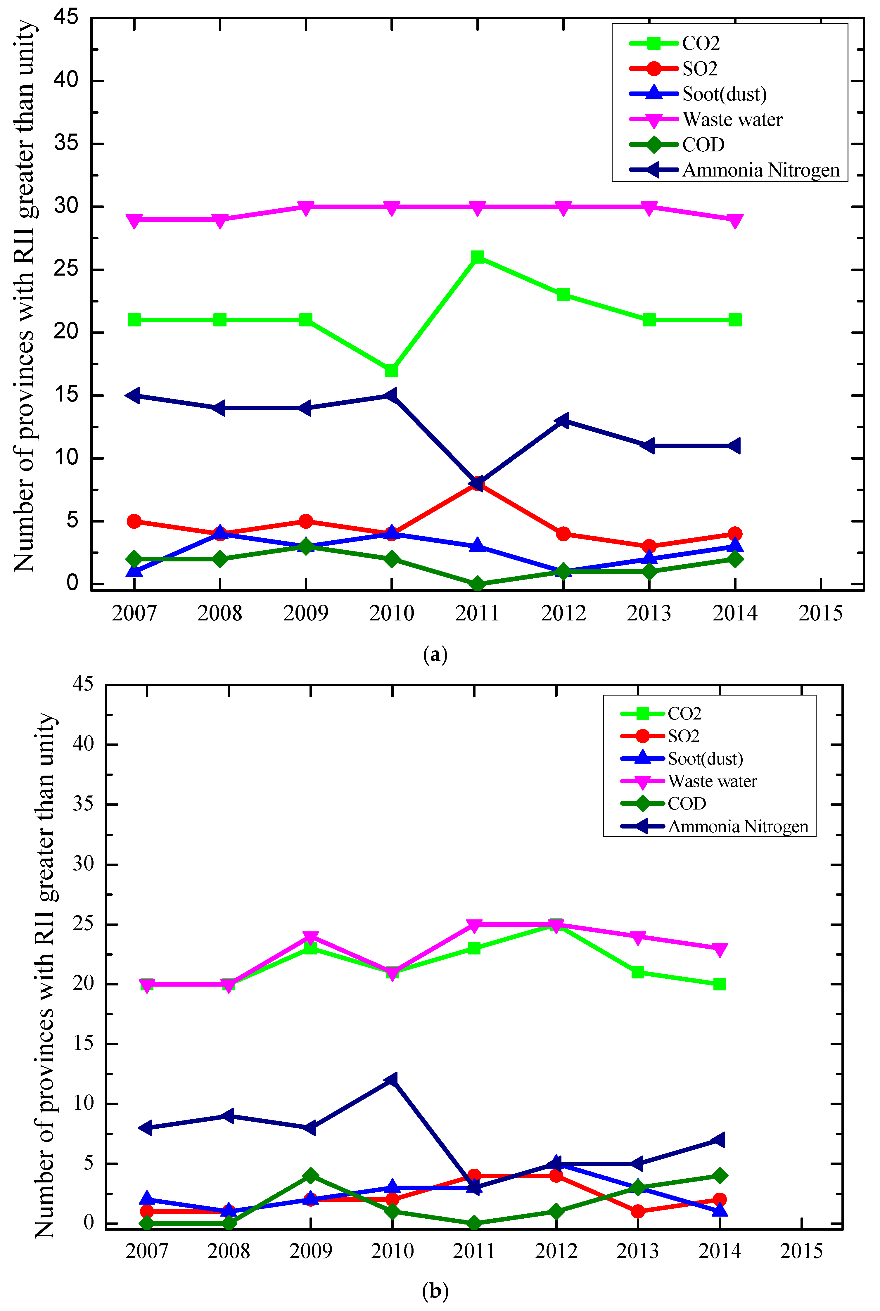
5.4.1. The Relative Efficiency Index of RII

Here, this study discusses the results of RII, which captures the relative efficiency of various pollutants in one given province.

Figure 7a,b present the number of provinces with an RII greater than unity under natural and managerial disposability, respectively. Figure 7a together with Figure 7b provides us the following concerns.

First, there are large differences across pollutants in the number of provinces with RII greater than unity under natural disposability. Consider the case of natural disposability as an example. During the analysis period, there are 29.63 provinces on average with number of provinces with RIIN greater than unity in terms of waste water. The number declines to 21.38 provinces in terms of CO₂, 12.63 in Ammonia Nitrogen, 4.63 in SO₂, 2.63 in soot and dust and 1.63 in COD. These results imply that most attention has been paid to waste water and CO₂. Considerable attention is given to Ammonia Nitrogen. However, little attention is given to other pollutants (i.e., SO₂, soot and dust and COD). There are similar results in the case of managerial disposability.

Second, the number of provinces with RII greater than unity remain stable during the analysis period. Meanwhile, there are considerable variations in certain time periods for some pollutants. Consider the case of natural disposability as an example. In terms of CO₂, there 21 provinces with RIIN greater than unity from 2007 to 2009. However, the number drops to 17 in 2010, increases to 26 in 2011 and then returns to 21 in 2013. As for SO₂, the number of provinces with RIIN greater than unity ranges from 3 to 5. However, the number increases to 8 in 2011.

Finally, there are considerable differences in the results between natural and managerial disposability. In terms of waste water, the number of provinces with RIIN greater than unity under natural disposability are greater than those of RIIM. There are similar results regarding Ammonia Nitrogen. These results imply that there should be differentiated policy direction of implementing social sustainability, when dealing with different pollutants.

5.4.2. The Relative Efficiency Index of RETI

Another efficiency index is RETI, which can be used to compare the performance across pollutants. Figure 8a illustrates the distribution of average RETIN values across provinces and Figure 8b illustrates the results of RETIM values.

Figure 8a combined with Figure 8b provides us the following concerns. First, there are significant differences across pollutants in the mean of RETI values. Consider the case of natural disposability as an example. There are three pollutants with the mean of average RETIN values greater than unity, i.e., waste water (1.056), CO₂ (1.013) and Ammonia Nitrogen (1.004). The mean of average RETIN values are less than unity for other pollutants, i.e., COD (0.991), SO₂ (0.991) and soot and dust (0.981).

Second, there are considerable differences across pollutants in the distribution of average RETI values. Consider the case of natural disposability as an example. Regarding waste water, most average RETI values are greater than unity and the distribution is like “M”-shaped. As for CO₂, average RETIN values are almost centered by unity and the values drop considerably from 1.10 to 0.95, forming “W”-shaped distribution. Things are similar in terms of COD and Ammonia Nitrogen. By comparison, the distribution is much scatter as for soot (dust) and SO₂.

Finally, there are considerable differences in the results between natural disposability and managerial disposability. Consider the mean of average RETI values as an example. Average RETIN values of Ammonia Nitrogen is greater than unity under natural disposability (1.004), implying that the efficiency is higher than the average levels. However, the values are less than unity under managerial disposability (0.996), and thus the efficiency is less than the average levels.

6. Conclusions

Recently, intermediate approach was proposed as a new approach, beyond the two conventional approaches (radial or non-radial approaches). It is a new approach with several unique important features and there are quite limited related studies. This study contributes to the DEA studies by putting forward an analytical framework of combining intermediate approach and DEA window analysis along with the concepts of natural and managerial disposability. This new approach is applied to evaluate China’s social sustainability, since China is a large transitional economy and faces serious environmental issues combined with complicated variations across provinces and pollutants. This study puts forward a series of performance indices from different angels. It provides the detailed information on the performance differences across provinces and across pollutants, which are useful and important for policy makers.

Our conclusions are threefold, which are as follows.

Firstly, more attention should be given to the concept of managerial disposability. According to the results, there exists a large potential for the Chinese provinces to improve efficiency based on the concept of managerial disposability. Such efficiency improvement can be achieved by eco-technology advancements and managerial efforts of business leaders and policy makers. Thus, these kind of efforts should play an important role in promoting social sustainability.

Secondly, there are large differences in the performance indices across provinces and across pollutants. The differences are in values and time trends of performance indices. It is noteworthy that geographical location is an important factor determining the performance. Meanwhile, there are significant differences in efficiency across pollutants, implying that different pollutants are treated differently by the Chinese governments. Looking ahead, the Chinese governments should give sufficient attention to the provinces and pollutants with poor performance.

In addition, more complicated performance indices are encouraged, since performance indices can provide useful information from different perspectives. Such information is quite important and useful for social sustainability assessment in China.

Finally, the Chinese government should reduce the provincial gaps and promote sustainable development. In the short term, the Chinese government can promote efficiency improvement by “catching up.” Effective policies should be adopted to encourage the local governments and business leaders to improve managerial performance and promote eco-technology advancements.

In the long term, the central government should reduce regional disparity to promote social sustainability. When “catching up” is implemented over time, the potential of efficiency improvement will become more and more limited. Then, there will be increasing difficulty in efficiency improvements in future. In this case, the central government should try to help the under-developed provinces to fulfill social sustainability. By reducing regional gaps, China can improve the level of social sustainability.

References

1. BP. Statistical Review of World Energy. 2017. Available online: http://www.bp.com/statisticalreview (accessed on 19 August 2017).
2. IEA. CO2 Emissions from Fuel Combustion, 2016th ed.; IEA: Paris, France; Available online: http://www.iea.org/publications/freepublications/publication/CO2EmissionsfromFuelCombustion_Highlights_2016.pdf (accessed on 16 August 2017).
3. National Bureau of Statistics of China. China Statistical Yearbook on Environment 2006–2015; China Statistics Press: Beijing, China, 2006–2015.
4. Yao, X.; Zhou, H.; Zhang, A.; Li, A. Regional energy efficiency, carbon emission performance and technology gaps in China: A meta-frontier non-radial directional distance function analysis. Energy Policy 2015, 84, 142–154. [Google Scholar] [CrossRef]
5. Li, A.; Peng, D.; Wang, D.; Yao, X. Comparing regional effects of climate policies promoting non-fossil fuels in China. Energy 2017, 141, 1998–2012. [Google Scholar] [CrossRef]
6. Li, A.; Zhang, A.; Zhou, Y.; Yao, X. Decomposition analysis of factors affecting carbon dioxide emissions across provinces in China. J. Clean. Prod. 2017, 141, 1428–1444. [Google Scholar] [CrossRef]
7. Zhang, Z.; Zhang, A.; Wang, D.; Li, A.; Song, H. How to improve the performance of carbon tax in China? J. Clean. Prod. 2017, 142, 2060–2072. [Google Scholar] [CrossRef]
8. Sueyoshi, T.; Goto, M. A comparative study among fossil fuel power plants in PJM and California ISO by DEA environmental assessment. Energy Econ. 2013, 40, 130–145. [Google Scholar] [CrossRef]
9. Sueyoshi, T.; Goto, M. DEA environmental assessment in a time horizon: Malmquist index on fuel mix, electricity and CO2 of industrial nations. Energy Econ. 2013, 40, 370–382. [Google Scholar] [CrossRef]
10. Sueyoshi, T.; Goto, M. Japanese fuel mix strategy after disaster of Fukushima Daiichi nuclear power plant: Lessons from international comparison among industrial nations measured by DEA environmental assessment in time horizon. Energy Econ. 2015, 52, 87–103. [Google Scholar] [CrossRef]
11. Sueyoshi, T.; Yuan, Y. Social sustainability measured by intermediate approach for DEA environmental assessment: Chinese regional planning for economic development and pollution prevention. Energy Econ. 2017, 66, 154–166. [Google Scholar] [CrossRef]
12. Sueyoshi, T.; Yuan, Y.; Li, A.; Wang, D. Social Sustainability of Provinces in China: A Data Envelopment Analysis (DEA) Window Analysis under the Concepts of Natural and Managerial Disposability. Sustainability 2017, 9, 2078. [Google Scholar] [CrossRef]
13. Charnes, A.; Cooper, W.W.; Rhodes, E. Measuring the efficiency of decision making units. Eur. J. Oper. Res. 1978, 6, 429–444. [Google Scholar] [CrossRef]
14. Cooper, W.W.; Seiford, L.M.; Zhu, J. Data Envelopment Analysis: History, Models, and Interpretations. In Handbook on Data Envelopment Analysis; Springer: Berlin, Germany, 2004; Volume 2, pp. 1–39. [Google Scholar]
15. Coelli, T.J.; Rao, D.S.P.; O’Donnell, C.J.; Battese, G.E. An Introduction to Efficiency and Productivity Analysis, 2nd ed.; Springer: New York, NY, USA, 2005. [Google Scholar]
16. Sueyoshi, T.; Goto, M. Environmental Assessment on Energy and Sustainability by Data Envelopment Analysi; John Wiley & Sons: London, UK, 2018; pp. 1–704. [Google Scholar]
17. Färe, R.; Grosskopf, S.; Norris, M.; Zhang, Z. Productivity Growth, Technical Progress, and Efficiency Change in Industrialized Countries. Am. Econ. Rev. 1994, 84, 66–83. [Google Scholar]
18. Barros, C.P.; Managi, S.; Matousek, R. The technical efficiency of the Japanese banks: Non-radial directional performance measurement with undesirable output. Omega 2012, 40, 1–8. [Google Scholar] [CrossRef]
19. Zhou, P.; Ang, B.W.; Wang, H. Energy and CO2 emission performance in electricity generation: A non-radial directional distance function approach. Eur. J. Oper. Res. 2012, 221, 625–635. [Google Scholar] [CrossRef]
20. Zhang, J.; Liu, Y.; Chang, Y.; Zhang, L. Industrial eco-efficiency in China: A provincial quantification using three-stage data envelopment analysis. J. Clean. Prod. 2017, 143, 238–249. [Google Scholar] [CrossRef]
21. Zhang, N.; Kong, F.; Choi, Y.; Zhou, P. The effect of size-control policy on unified energy and carbon efficiency for Chinese fossil fuel power plants. Energy Policy 2014, 70, 193–200. [Google Scholar] [CrossRef]
22. Zhang, Y.J.; Hao, J.F.; Song, J. The CO2 emission efficiency, reduction potential and spatial clustering in China’s industry: Evidence from the regional level. Appl. Energy 2016, 174, 213–223. [Google Scholar] [CrossRef]
23. Tapia, J.; Promentilla, M.; Tseng, M.; Tan, R. Screening of carbon dioxide utilization options using hybrid Analytic Hierarchy Process-Data Envelopment Analysis method. J. Clean. Prod. 2017, 165, 1361–1370. [Google Scholar] [CrossRef]
24. Liu, X.; Chu, J.; Yin, P.; Sun, J. DEA cross-efficiency evaluation considering undesirable output and ranking priority: A case study of eco-efficiency analysis of coal-fired power plants. J. Clean. Prod. 2017, 142, 877–885. [Google Scholar] [CrossRef]
25. Bi, G.; Shao, Y.; Song, W.; Yang, F.; Luo, Y. A performance evaluation of China’s coal-fired power generation with pollutant mitigation options. J. Clean. Prod. 2018, 171, 867–876. [Google Scholar] [CrossRef]
26. Zhou, P.; Sun, Z.R.; Zhou, Q. Optimal path for controlling CO2 emissions in China: A perspective of efficiency analysis. Energy Econ. 2014, 45, 99–110. [Google Scholar] [CrossRef]
27. Sueyoshi, T.; Yuan, Y.; Li, A.; Wang, D. Methodological Comparison among Radial, Non-radial and Intermediate Approaches for DEA Environmental Assessment. Energy Econ. 2017, 67, 439–453. [Google Scholar] [CrossRef]
28. Bowlin, W.F. Evaluating the Efficiency of US Air Force Real-Property Maintenance Activities. J. Oper. Res. Soc. 1987, 38, 127–135. [Google Scholar] [CrossRef]
29. Thore, S.; Kozmetsky, G.; Phillips, F. DEA of Financial Statements Data: The U.S. Computer Industry. J. Product. Anal. 1994, 5, 229–248. [Google Scholar] [CrossRef]
30. Goto, M.; Tsutsui, M. Comparison of Productive and Cost Efficiencies among Japanese and US Electric Utilities. Omega 1998, 26, 177–194. [Google Scholar] [CrossRef]
31. Sueyoshi, T.; Aoki, S. A use of a nonparametric statistic for DEA frontier shift: The Kruskal and Wallis rank test. Omega 2001, 29, 1–18. [Google Scholar] [CrossRef]
32. Yang, W.C.; Lee, Y.M.; Hu, J.L. Urban sustainability assessment of Taiwan based on data envelopment analysis. Renew. Sustain. Energy Rev. 2016, 61, 341–353. [Google Scholar] [CrossRef]
33. Vlontzos, G.; Pardalos, P.M. Assess and prognosticate green house gas emissions from agricultural production of EU countries, by implementing, DEA Window analysis and artificial neural networks. Renew. Sustain. Energy Rev. 2017, 76, 155–162. [Google Scholar] [CrossRef]
34. Bian, Y.W.; Yang, F. Resource and environment efficiency analysis of provinces in China: A DEA approach based on Shannon’s entropy. Energy Policy 2010, 38, 1909–1917. [Google Scholar] [CrossRef]
35. Guo, X.D.; Zhu, L.; Fan, Y.; Xie, B.C. Evaluation of potential reductions in carbon emissions in Chinese provinces based on environmental DEA. Energy Policy 2011, 39, 2352–2360. [Google Scholar] [CrossRef]
36. Wang, K.; Wei, Y.M.; Zhang, X. A comparative analysis of China’s regional energy and emission performance: Which is the better way to deal with undesirable outputs? Energy Policy 2012, 46, 574–584. [Google Scholar] [CrossRef]
37. Wu, F.; Fan, L.W.; Zhou, P.; Zhou, D.Q. Industrial energy efficiency with CO2 emissions in China: A nonparametric analysis. Energy Policy 2012, 49, 164–172. [Google Scholar] [CrossRef]
38. Wang, Q.W.; Zhao, Z.Y.; Zhou, P.; Zhou, D.Q. Energy efficiency and production technology heterogeneity in China: A meta-frontier DEA approach. Econ. Model. 2013, 35, 283–289. [Google Scholar] [CrossRef]
39. Wang, K.; Wei, Y.M. China’s regional industrial energy efficiency and carbon emissions abatement costs. Appl. Energy 2014, 130, 617–631. [Google Scholar] [CrossRef]
40. Wang, Z.H.; Feng, C.; Zhang, B. An empirical analysis of China’s energy efficiency from both static and dynamic perspectives. Energy 2014, 74, 322–330. [Google Scholar] [CrossRef]
41. Wu, J.; An, Q.X.; Yao, X.; Wang, B. Environmental efficiency evaluation of industry in China based on a new fixed sum undesirable output data envelopment analysis. J. Clean. Prod. 2014, 74, 96–104. [Google Scholar] [CrossRef]
42. Li, K.; Lin, B.Q. Metafroniter energy efficiency with CO2 emissions and its convergence analysis for China. Energy Econ. 2015, 48, 230–241. [Google Scholar] [CrossRef]
43. Du, H.B.; Matisoff, D.C.; Wang, Y.Y.; Liu, X. Understanding drivers of energy efficiency changes in China. Appl. Energy 2016, 184, 1196–1206. [Google Scholar] [CrossRef]
44. Long, R.Y.; Wang, H.Z.; Chen, H. Regional differences and pattern classifications in the efficiency of coal consumption in China. J. Clean. Prod. 2016, 112, 3684–3691. [Google Scholar] [CrossRef]
45. Sueyoshi, T.; Yuan, Y. Returns to damage under undesirable congestion and damages to return under desirable congestion measured by DEA environmental assessment with multiplier restriction: Economic and energy planning for social sustainability in China. Energy Econ. 2016, 56, 288–309. [Google Scholar] [CrossRef]
46. Wu, J.; Yin, P.Z.; Sun, J.S.; Chu, J.F.; Liang, L. Evaluating the environmental efficiency of a two-stage system with undesired outputs by a DEA approach: An interest preference perspective. Eur. J. Oper. Res. 2016, 254, 1047–1062. [Google Scholar] [CrossRef]
47. Chen, L.; Jia, G.Z. Environmental efficiency analysis of China’s regional industry: A data envelopment analysis (DEA) based approach. J. Clean. Prod. 2017, 142, 846–853. [Google Scholar] [CrossRef]
48. Chen, L.; Wang, Y.; Lai, F.; Feng, F. An investment analysis for China’s sustainable development based on inverse data envelopment analysis. J. Clean. Prod. 2017, 142, 1638–1649. [Google Scholar] [CrossRef]
49. Du, J.; Chen, Y.; Huang, Y. A Modified Malmquist-Luenberger Productivity Index: Assessing Environmental Productivity Performance in China. Eur. J. Oper. Res. 2017, in press. [Google Scholar] [CrossRef]
50. Feng, C.; Zhang, H.; Huang, J.B. The approach to realizing the potential of emissions reduction in China: An implication from data envelopment analysis. Renew. Sustain. Energy Rev. 2017, 71, 859–872. [Google Scholar] [CrossRef]
51. Wang, Z.; He, W. Regional energy intensity reduction potential in China: A non-parametric analysis approach. J. Clean. Prod. 2017, 149, 426–435. [Google Scholar] [CrossRef]
52. Song, M.; Peng, J.; Wang, J.; Zhao, J. Environmental efficiency and economic growth of China: A Ray slack-based model analysis. Eur. J. Oper. Res. 2017, in press. [Google Scholar] [CrossRef]
53. Zhu, Q.; Wu, J.; Li, X.; Xiong, B. China’s regional natural resource allocation and utilization: A DEA-based approach in a big data environment. J. Clean. Prod. 2017, 142, 809–818. [Google Scholar] [CrossRef]
54. National Bureau of Statistics of China. China Energy Statistical Yearbook 2006–2016; China Statistics Press: Beijing, China, 2006–2016.
55. National Bureau of Statistics of China. China Statistical Yearbook 2006–2016; China Statistics Press: Beijing, China, 2006–2016.
56. Sueyoshi, T.; Goto, M. Undesirable congestion under natural disposability and desirable congestion under managerial disposability in U.S. electric power industry measured by DEA environmental assessment. Energy Econ. 2016, 55, 173–188. [Google Scholar] [CrossRef]
57. Färe, R.; Grosskopf, S.; Lovell, C.A.K.; Pasurka, C. Multilateral productivity comparisons when some outputs are undesirable: A nonparametric approach. Rev. Econ. Stat. 1989, 71, 90–98. [Google Scholar] [CrossRef]
58. Sueyoshi, T.; Goto, M. Data envelopment analysis for environmental assessment: Comparison between public and private ownership in petroleum industry. Eur. J. Oper. Res. 2012, 216, 668–678. [Google Scholar] [CrossRef]
59. Sueyoshi, T.; Goto, M. DEA environmental assessment of coal fired power plants: Methodological comparison between radial and non-radial models. Energy Econ. 2012, 34, 1854–1863. [Google Scholar] [CrossRef]
60. Sueyoshi, T.; Goto, M. DEA radial and non-radial models for unified efficiency under natural and managerial disposability: Theoretical extension by strong complementary slackness conditions. Energy Econ. 2012, 34, 700–713. [Google Scholar] [CrossRef]
61. Sueyoshi, T.; Goto, M. DEA radial measurement for environmental assessment: A comparative study between Japanese chemical and pharmaceutical firms. Appl. Energy 2014, 115, 502–513. [Google Scholar] [CrossRef]
62. Sueyoshi, T.; Goto, M. Environmental assessment for corporate sustainability by resource utilization and technology innovation: DEA radial measurement on Japanese industrial sectors. Energy Econ. 2014, 46, 295–307. [Google Scholar] [CrossRef]
63. Sueyoshi, T.; Yuan, Y. China’s regional sustainability and diversified resource allocation: DEA environmental assessment on economic development and air pollution. Energy Econ. 2015, 49, 239–256. [Google Scholar] [CrossRef]
64. Sueyoshi, T.; Yuan, Y. Marginal Rate of Transformation and Rate of Substitution measured by DEA environmental assessment: Comparison among European and North American nations. Energy Econ. 2016, 56, 270–287. [Google Scholar] [CrossRef]
65. Sueyoshi, T.; Goto, M. DEA approach for unified efficiency measurement: Assessment of Japanese fossil fuel power generation. Energy Econ. 2011, 33, 292–303. [Google Scholar] [CrossRef]
66. Shan, H. Reestimating the capital stock in China: 1952–2006. J. Quant. Tech. Econ. 2008, 10, 17–31. (In Chinese) [Google Scholar]
67. China Economic and Social Development Statistics Database. 2017. Available online: http://tongji.cnki.net/kns55/index.aspx (accessed on 10 February 2017).
68. National Bureau of Statistics of China. China Labour Statistical Yearbook 2006–2015; China Statistics Press: Beijing, China, 2006–2015.
69. National Bureau of Statistics of China. 2017. Available online: http://data.stats.gov.cn/easyquery.htm?cn=E0103 (accessed on 13 February 2017).
70. Du, L.M. Impact Factors of China’s Carbon Dioxide Emissions: Provincial Panel Data Analysis. South China J. Econ. 2010, 11, 20–33. (In Chinese) [Google Scholar]
71. IPCC. IPCC Guidelines for National Greenhouse Gas Inventories. 2006. Available online: https://www.ipcc-nggip.iges.or.jp/public/2006gl/ (accessed on 15 February 2017).
72. National Coordination Committee on Climate Change; Energy Research Institute of National Development and Reform Commission. Study on GHG inventories in China; China Environmental Science Press: Beijing, China, 2007.
Figure 1. Energy intensity across provinces in China in 2015. Sources: [54,55]. Note: China’s provinces and their abbreviations are as follows and hereafter in this paper. BJ, Beijing; TJ, Tianjin; HEB, Hebei; SX, Shanxi; IM, Inner Mongolia; LN, Liaoning; JL, Jilin; HLJ, Heilongjiang; SH, Shanghai; JS, Jiangsu; AH, Anhui; CQ, Chongqing; FJ, Fujian; GS, Gansu; GD, Guangdong; GX, Guangxi; GZ, Guizhou; HAN, Hainan; HEN, Henan; HUB, Hubei; HUN, Hunan; JX, Jiangxi; NX, Ningxia; QH, Qinghai; SAX, Shaanxi; SC, Sichuan; YN, Yunnan; SD, Shandong; XJ, Xinjiang; ZJ, Zhejiang. For simplicity, this study does not cover all geographical regions of China and South China Sea and other related regions are not included in the maps (hereafter in this study).
Sustainability 10 00732 g001
Figure 2. GRP and structure of economy across provinces in China in 2015. Sources: [55]. Note: GRP1, GRP2 and GRP3 stand for primary industry, secondary industry and tertiary industry respectively.
Sustainability 10 00732 g002
Figure 3. Average UEIN values across provinces in China.
Sustainability 10 00732 g003
Figure 4. Average UEIM values across provinces in China.
Sustainability 10 00732 g004
Figure 5. Average BPIN values across provinces in China.
Sustainability 10 00732 g005
Figure 6. Average BPIM values across provinces in China.
Sustainability 10 00732 g006
Figure 7. (a) Number of provinces with RIIN greater than unity; (b) Number of provinces with RIIM greater than unity.
Sustainability 10 00732 g007
Figure 8. (a) Distribution of average RETIN values; (b) Distribution of average RETIM values.
Sustainability 10 00732 g008