The US Shale Gas Revolution and Its Externality on Crude Oil Prices: A Counterfactual Analysis

Abstract

The expansion of shale gas production since the mid-2000s which is commonly referred to as “shale gas revolution” has had large impacts on global energy outlook. The impact is particularly substantial when it comes to the oil market because natural gas and oil are substitutes in consumption and complements and rivals in production. This paper investigates the price externality of shale gas revolution on crude oil. Applying a structural vector autoregressive model (VAR) model, the effect of natural gas production on real oil price is identified in particular, and then based on the identification, counterfactuals of oil price without shale gas revolution are constructed. We find that after the expansion of shale gas production, the real West Texas Intermediate (WTI) oil price is depressed by 10.22 USD/barrel on average from 2007 to 2017, and the magnitude seems to increase with time. In addition, the period before shale gas revolution is used as a “thought experiment” for placebo study. The results support the hypothesis that real WTI oil price can be reasonably reproduced by our models, and the estimated gap for oil price during 2007–2017 can be attributed to shale gas revolution. The methodology and framework can be applied to evaluate the economic impacts of other programs or policies.

1. Introduction

Over the past several years, unconventional gas has gained centre stage in the global energy market, which is mainly driven by rapid development in the US shale gas production [1]. Previously, the viability of shale gas was regarded as either non-feasible or uneconomical due to technological limitations and low gas price. However, during the mid-2000s, the application of hydraulic fracturing and horizontal drilling in the US, coupled with the surge in gas prices, enabled the extraction of huge quantities of natural gas from shale [2]. The production of shale gas has therefore increased thirteen times between 2007 and 2016. In 2016, shale gas output was 17,032 billion cubic feet (Bcf), which was more than twice the total energy consumption of China in that year (7268 Bcf). The proportion of shale gas production in total US natural gas production increased from 2.2% in 2000 to 52.2% in 2016.

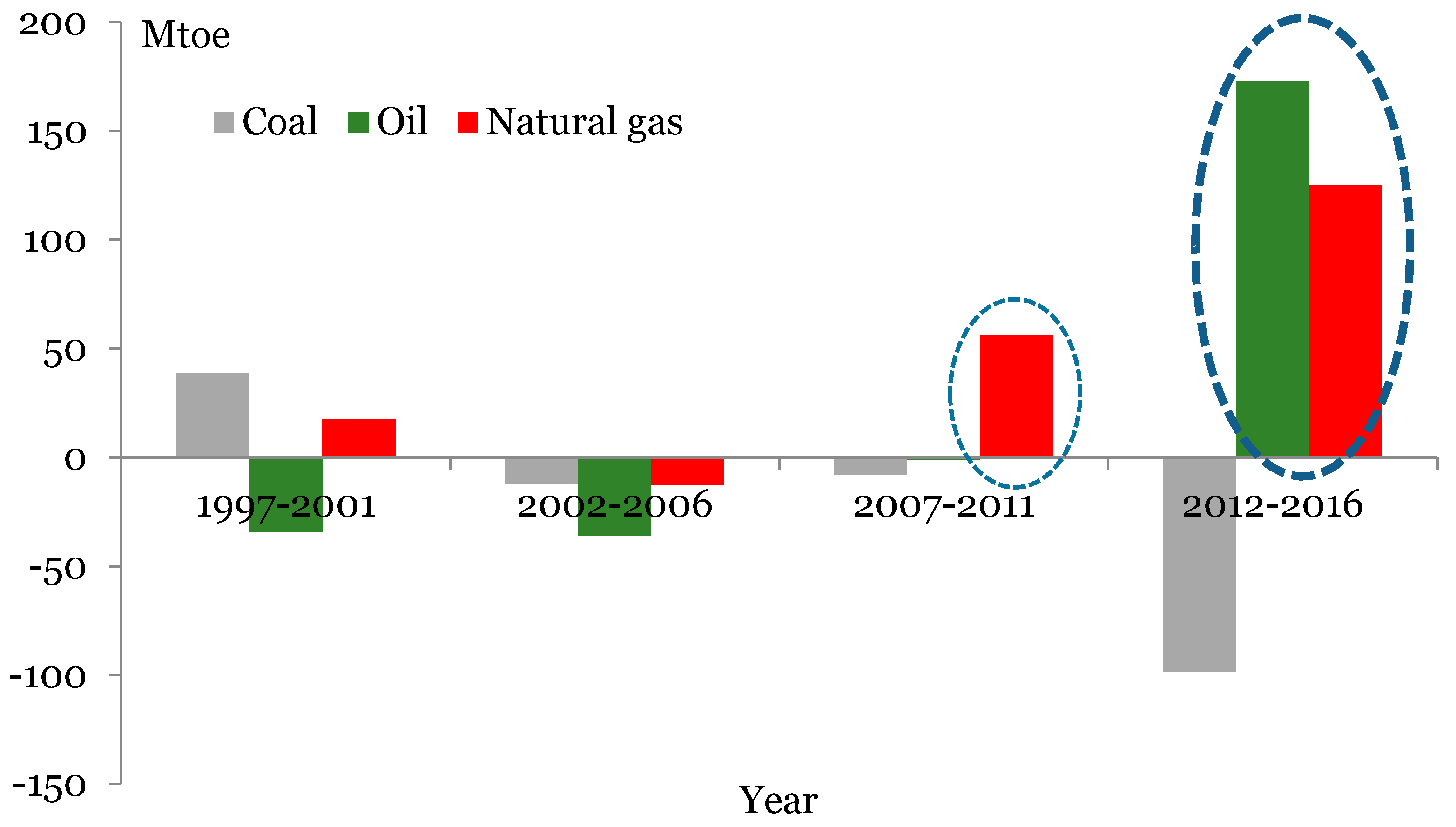
The huge extraction of shale gas has not only offset the decline in conventional gas production, but also has led to a dramatic increase in total natural gas output. Figure 1 depicts the changes in the production of coal, crude oil and natural gas in each five year periods since early 1990s. As Figure 1 shows, the rapid growth of natural gas production from shale gas after mid-2000s alone with shale oil boom after 2010s are the biggest energy stories in energy production over the last two decades. As Dr. Daniel Yergin claims, “the rapidity and sheer scale of the shale breakthrough—and its effects on markets—qualified it as the most significant innovation in energy so far since the start of the 21st century” [3]. In order to focus on shale gas revolution, the impact of shale oil boom will be controlled in the counterfactual analysis later

The notable growth of shale gas has not only radically changed the energy landscape in the US, but also in the world, such as competing with coal in electricity generation [4], and redirecting of recent growth in liquefied natural gas (LNG) supply to Europe and Asia [5]. When it comes specifically to the oil market, the shale gas revolution brings down the price of crude oil. Due to the limitation of US energy policy and export capacity, the oversupply from shale gas in the US is dragging down the price of natural gas. Crude oil and natural gas are substitutes in consumption [6], factories and other consumers would shift energy input from oil to natural gas when the relative price of each energy type changes. 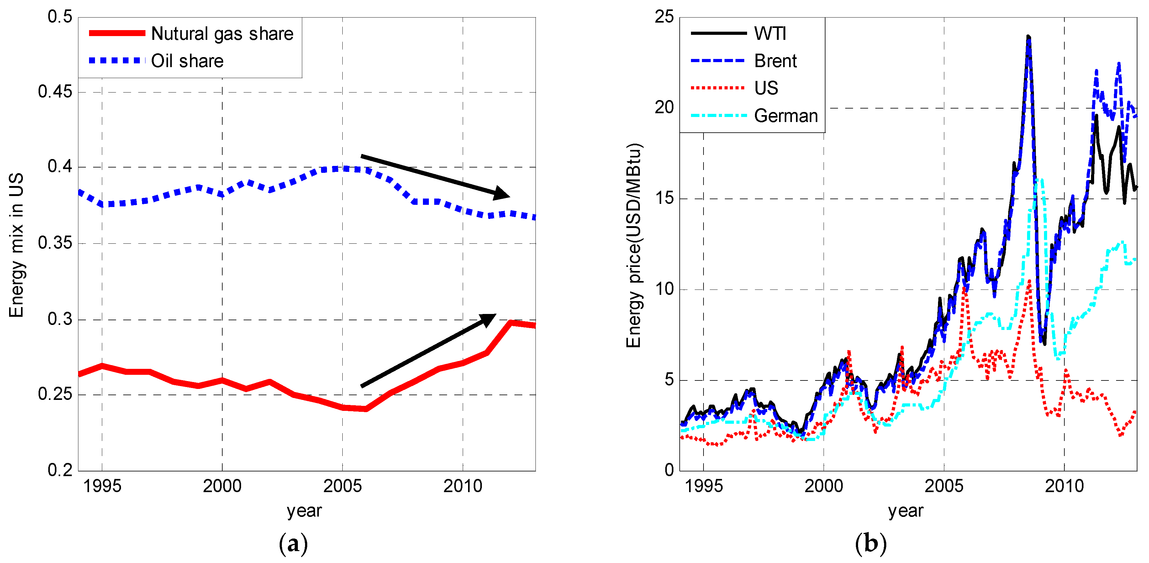Since natural gas is cheap in the US due to shale gas expansion, the demand for oil might decrease due to its substitution by natural gas through competition [7]. Therefore, the price of oil would also be plunged by shale gas boom. This mechanism described above is captured in Figure 2. Figure 2a shows the energy mix in the US between 1994–2013. Since the mid-2000s, with the production surge in shale gas, the share of natural gas has increased gradually and the share of oil in the energy mix has declined correspondingly, indicating that natural gas is substituting oil in energy consumption. Figure 2b depicts the trend of natural gas prices in US and Germany, and the West Texas Intermediate (WTI) and Brent crude oil prices. The German natural gas prices are presented to compare natural gas prices of the US which is under intervention of shale gas revolution and natural gas prices of Germany which has no shale gas intervention. In order to make the prices of natural gas and oil comparable, all prices are converted to US dollar(USD)/MBtu by conversion factors. Here, one thousand cubic feet of natural gas equals to 1.03 MBtu, and 1 barrel of crude oil equals to 5.6 MBtu). As shown in Figure 2b, the spread between WTI and Brent crude oil prices is considerably large in recent years. WTI crude oil price represents the prices that oil producers received in the US and Brent represents the prices received internationally. Thus, it might be the expansion of shale gas in the US that lowers WTI price substantially because natural gas and crude oil are substitutes in consumption and shale gas expansion only occurred in the US (recall that WTI is the prices that oil producers received in the U.S.). This paper provides empirical evidence for this assumption.

The rapid development of shale gas is believed to have strong adverse effects on oil price. But, to date, the evidence on the assertion is scarce, probably because it is difficult to measure how oil price would have evolved in the absence of shale gas revolution. The objective of this paper is to assess the impact of shale gas revolution on crude oil price. This type of research is difficult using conventional econometric modeling because the comparison of the evolution of oil price before and after the shale gas revolution will be contaminated by other shocks which affect the oil market during the sample periods. For example, a surge in real economic activity before 2007 contributed to the sustained rise in the price of oil [8]. While the collapse of oil price after the financial crisis in 2008 appears to be driven mainly by the speculation of traders [9]. Therefore, a simple comparison of the evolution of oil price before and after shale gas revolution would not only contain the effect of shale gas but also the effects of other factors, such as oil supply, economic activity and oil market specific shocks.

Our empirical research builds on previous studies by identifying the shocks of shale gas production on oil price and constructing the counterfactuals of oil price in absence of shale gas expansion. Intuitively, if one knows the outcomes of oil price under intervention of shale gas revolution and under no-intervention, the impact of shale gas revolution on oil price is just the difference between oil prices with shale gas and in the absence of shale gas. One of the difficulties in measuring the impact of shale gas is not being able to simultaneously observe the time series of oil prices under the intervention of shale gas and under no-intervention. What we observed is the oil price under the intervention of shale gas, while the price if there is no shale gas is unobservable. To properly evaluate the impact of shale gas revolution on oil price, we need to construct the counterfactuals of oil price if there is no shale gas.

Assuming that shale gas begins to impact the oil price dramatically since time $T$, our approach to construct the counterfactuals of oil price in $t\ge T$ without the intervention of shale gas, is to use the relationship of observations that have not yet been subject to intervention, say $t<T$, to predict what the oil price in $t\ge T$ would have evolved had it not been subject to shale gas revolution. The basic idea behind this approach is that time series with observations before shale gas revolution would often contain information on how the price of oil reacts to shocks in natural gas production. If the reactions of oil price towards production changes in natural gas are similar, information about the impact of natural gas production on oil price could help to constructs the counterfactuals of oil price after shale gas revolution [10].

Specifically, we investigate the impact of shale gas on oil price using two procedures. First, structural vector autoregressive model (SVAR) is applied to identify the shocks in natural gas production on oil price. Naturally, the changes in natural gas production exhibit similar effects on oil price before and after shale gas revolution. Second, we eliminate the effects of supply shocks and construct the counterfactuals of oil price in the absence of shale gas expansion. The magnitude of shale gas impact on oil price is the gap between the actual price and the counterfactuals. In addition, the reliability of our analysis depends on whether the counterfactuals could reproduce the historical path of oil price in the absence of shale gas revolution. To address this question, we further perform a “placebo study”. The idea is to compare the evolution of oil price in the period with negligible shale gas production to its counterfactual version. We therefore apply the two procedures above to compute the oil price series in the period between 2004 and 2006 when shale gas production is negligible.

The rest of this paper is organized as follows. Section 2 briefly presents an overview of studies on shale gas and counterfactual analysis. Section 3 discusses the SVAR framework and its identification, in which we specifically focus on identifying the impacts of shocks in natural gas production on oil price and the method to construct the counterfactuals. In Section 4, we present the empirical results about the counterfactuals and the effects of shale gas revolution on oil price. Next, a placebo study is applied in Section 5. The final section concludes the study.

2. Literature Review

The discussions on the expansion of shale gas production were increased rapidly a decade ago. Most literature in the early stage on shale gas have been limited to estimating the scale of the global resource of unconventional gas. For example, IEA [11] provides a review of the historic growth of US unconventional gas and evaluates the potential of global shale gas development; IEA [12] introduces for the first time the “Golden Age of Gas” in the World Energy Outlook. Similar studies include Medlock [13] and McGlade et al. [14]. Most of them show that shale gas resource might potentially be very large and of good quality, although the range of uncertainty is still extremely wide (such as Hilaire et al. [15]; Kim and Lee [16]).

The shale gas boom over the last decade has generated growing interest in studying the impacts of shale gas extraction on energy market and economic activity. In general, literatures on these issues are relatively rare but rapidly growing. Existing literature on the effects of shale gas tend to be divided into two categories: its economic impacts, and its impacts on the energy market.

The economic effects of rapid shale gas development such as stimulating economic expansion, creating job and expanding energy intensive manufacturing in US have been profound [17]. Kinnaman [18], Wang et al. [17] and Yuan et al. [19] provide informative reviews of these studies. To be more specific, Bonakdarpour et al. [20] suggests that the shale gas industry contributed more than 600,000 jobs in 2010 and is likely to increase to around 870,000 by 2015 and more than 1.6 million by 2035. Muehlenbachs et al. [21] analyze the impacts of shale gas development on housing markets. Munasib and Rickman [22] examine the net economic impacts of oil and gas production from shale formations for key shale oil and gas producing areas. Other relevant studies could be seen in Considine et al. [23], Weber [24], and Hartley et al. [25].

Shale gas could transform the landscape of global energy market by lowering gas price, introducing a new composition of energy mix and changing the current energy flows [26]. The US shale gas expansion adds production to the well-supplied gas market, and gas price in the US has plummeted. Erdős [27] find that the US gas price has decoupled from crude oil price after shale gas expansion due to the oversupply from US shale gas output. In power generation, coal fired power is being displaced by the rise in the availability of shale gas [1]. Melikoglu [28] analyzes the role of shale gas in the global energy market, and concludes that it will have an increased share of natural gas in energy mix and probably lead to the decline in natural gas price. Gilbert and Sovacool [29] claim that shale gas provides a better modelling for the low-carbon energy system because it can complement with renewable energy by acting as a backup or coupling with energy storage.

In addition, by re-directing the trade flows of energy, shale gas changes the geography of the global energy market [5]. For example, Ebinger et al. [30] and Rogers [5] study the impact of shale gas on LNG markets and trade; O’Sullivan [31] investigates its impact on European markets and trade with Russia. Wang and Lin [32] study the impacts of unconventional gas development on China’s natural gas supply and energy price reform under different scenarios. They predict that the expansion of China’s unconventional gas would delay the gas production peak from middle 2020s to early 2040s.

Surprisingly, literature on the impact of shale gas revolution on oil price remains rather sparse and is mainly represented by Asche et al. [33]. They indicate that cheap gas driven by shale gas revolution would lower oil price because a substantial degree of substitution exists between oil and natural gas. Although they examine the long-term relationship between natural gas price and oil price, it is still unclear what magnitude the shale gas expansion has changed the evolution of oil price. Kilian [34] examines the impact of the shale oil revolution on US oil and gasoline prices. To the best of our knowledge, the study presented in our paper is unique in the literature on energy markets as it evaluates quantitatively the magnitude of the impact of shale gas revolution on oil price.

3. Methods

The analysis in this paper relies on identifying the impulse of natural gas production on oil price, and then the counterfactuals of real oil price without the production of shale gas could be constructed by extracting this impulse driven by shale gas revolution. The subsequent evolution of counterfactual oil price is compared with the actual price to evaluate the impact of shale gas revolution on real oil price.

3.1. A Structural VAR Model for the Determinants of Oil Price

Existing studies show that the price of oil is endogenous with respect to factors such as supply and demand in the energy market [8,9]. In this sub-section, we apply the structural VAR model to investigate how the price of oil is driven by the components of interest. Following Kilian [8], three components driving oil price is proposed: shocks to crude oil supply, global oil demand shocks and demand shocks that are specific to oil market (such as precautionary demand shock). In addition, given that natural gas production could affect the endogenous oil price, the production of natural gas has been particularly regarded as a factor that drives the evolution of oil price. Employing the structural VAR model, the response of oil price to the changes in natural gas production could be obtained, and it is the foundation of constructing the counterfactuals without shale gas revolution.

The aim of this sub-section is to identify how the changes in natural gas production drive oil price. To do that, one needs to identify the four shocks in structural VAR model from data, which can be specified as follows.

Let $x_t=\left(opro{d}_t,ngpro{d}_t,eco{n}_t,rp{o}_t\right)\prime$ denotes a $4\times 1$ vector of variables to be investigated, where $opro{d}_t$ denotes the global crude oil production, $ngpro{d}_t$ refers to production of natural gas, $eco{n}_t$ is the real economic activity, and $rp{o}_t$ denotes the real price of oil. A reduced VAR model for $x_t$ is given by:

$$C\left(L\right)x_t=e_t,C_0=I,E\left(e_t{e}_t\prime \right)=\mathsf{\Sigma }$$

(1)

where $C\left(L\right)$ is a polynomial lag operator, e.g., $L^s{x}_t=x_{t-s}$, and $e_t$ is a $4\times 1$ vector of linear forecast errors of $x_t$ with variance-covariance matrix $\mathsf{\Sigma }$. Equation (1) is a reduced-form and lacks structural economic interpretation. The objective of the structural VAR analysis is to propose economic restrictions to infer these structural relations from consistent estimation of $C\left(L\right)$ and $\mathsf{\Sigma }$.

Therefore, what is of interest to our analysis is the set of structural relations leading to Equation (1). Assuming that $A_0$ has a structure which could make the reduced-form errors $e_t$ be decomposed as:

$$e_t=A_0{}^{-1}{\epsilon }_t,E\left({\epsilon }_t{\epsilon }_t\prime \right)=\mathsf{\Omega }=diag\left({\omega }_j^2\right)$$

(2)

where ${\epsilon }_t$ denotes the $4\times 1$ vector of structural innovations which are serially and mutually uncorrelated by assumptions. The matrix $A_0$ identifies the relationships among the four variables in the system, which indicates the restrictions on the covariance structure of the VAR innovations in Equation (3):

$$\mathsf{\Sigma }=A_0^{-1}\mathsf{\Omega }{A}_0^{-1}\prime$$

(3)

In the structural VAR model, the number of parameters in $A_0$ and $\mathsf{\Omega }$ needs to be estimated is $n\left(n+1\right)$ (in our case $n=4$), while there are only $n\left(n+1\right)/2$ parameters in $\mathsf{\Sigma }$. It should be noted that we do not have sufficient prior information to set restrictions for ${\omega }_j^2$’s of $\mathsf{\Omega }$. Therefore, in order to identify the model, we need to impose $n\left(n+1\right)/2$ restrictions on $A_0$. $n$ restrictions have been given by normalizing the diagonal elements in $A_0$ to unity, leaving $n\left(n-1\right)/2$ restrictions in $A_0$ to be imposed.

In the present paper $n=4$, thus $n\left(n-1\right)/2=6$ restrictions are needed for identification of the four structural shocks. Similar to the identification specified in Kilian [8], we suppose that $A_0^{-1}$ has a recursive structure such that the structural shocks could be decomposed to VAR innovations according to:

$$e_t=\left(\begin{array}{l}{e}_t^{oprod}\\ e_t^{ngprod}\\ e_t^{econ}\\ e_t^{rpo}\end{array}\right)=\left(\begin{array}{cccc}1& 0& 0& 0\\ \alpha & 1& 0& 0\\ \beta & \varphi & 1& 0\\ \rho & \mu & \gamma & 1\end{array}\right)\left(\begin{array}{l}{\epsilon }_t^{os}\\ {\epsilon }_t^{ngs}\\ {\epsilon }_t^{ed}\\ {\epsilon }_t^{osd}\end{array}\right)$$

(4)

where ${\epsilon }_t^{os}$ denotes oil supply shock, ${\epsilon }_t^{ngs}$ denotes natural gas supply shock, ${\epsilon }_t^{ed}$ is economic demand shock, ${\epsilon }_t^{osd}$ is oil specific demand shock. The lower triangular matrix $A_0^{-1}$ provides the six necessary restrictions for the structural identification.

The restrictions imposed in Equation (4) are reasonable for the following reasons. First, given the uncertainty about the crude oil market and the costs of adjusting oil production, oil suppliers might be slow to respond to either natural gas supply shocks, demand shocks or oil price shocks. Therefore, the supply curve of crude oil in the short run (within a month) is vertical. It is worth noting that shocks in natural gas supply, aggregate demand or oil price would shift the short run vertical supply curve of oil with a delay of over a month. This would suggest the following contemporaneous relation:

$$e_t^{oprod}={\epsilon }_t^{os}$$

(5)

Second, due to similar reasons, the supply of natural gas is sluggish within the same month with respect to the shocks of aggregate demand and oil price. But natural gas and oil are somewhat complements in production, as shifts in oil supply might result in changes in natural gas production as a co-product of oil. Geologically, there are two basic forms for natural gas, e.g., associated gas and non-associated gas. The former refers to natural gas that occurs in crude oil reservoirs and its share in total gas production in the US in 2011 is about 21%. The natural gas production therefore would be effected by oil supply shocks. The relation for the aggregate demand structural shock is therefore given as:

$$e_t^{ngprod}=\alpha {\epsilon }_t^{os}+{\epsilon }_t^{ngs}$$

(6)

Third, the model imposes the restriction that global economic activity will not be lowered immediately by the increases in oil price driven by shocks that are specific to the oil market, such as increase in precautionary demand. This restriction is consistent with the delayed response of global economic activity after each of the major oil price increases. In terms of structural shocks this would imply the following identification:

$$e_t^{econ}=\beta {\epsilon }_t^{os}+\varphi {\epsilon }_t^{ngs}+{\epsilon }_t^{ed}$$

(7)

Finally, the real price of oil are partly endogenous, structural shocks to the real oil price which cannot be explained by the impacts of oil supply, natural gas supply and global economic activity are reflected in the shocks that are specific to oil market, such as fluctuations in precautionary demand for oil due to oil supply uncertainty in the future. According to Kilian [8], geopolitical effect can be reflected by shocks to supply (such as oil supply disruptions in Middle East) and market-specific shocks because geopolitical event might increase precautionary demand. Therefore, geopolitical effect has been incorporated in the ${\epsilon }_t^{os}$, ${\epsilon }_t^{ngs}$, and ${\epsilon }_t^{osd}$. Hence, in terms of structural shocks, this implies the following relation:

$$e_t^{rpo}=\rho {\epsilon }_t^{os}+\mu {\epsilon }_t^{ngs}+\gamma {\epsilon }_t^{ed}+{\epsilon }_t^{osd}$$

(8)

Based on the identification of the structural relations, the structural VAR model could be estimated considering the restrictions in Equations (5)–(8). However, the parameter estimations of either $C\left(L\right)$, $\mathsf{\Sigma }$ or $A_0$, $\mathsf{\Omega }$ may not tell us the interactions between the variables of interest. What is often of interest is to analyze the response of one variable to an impulse in another variable that further involves the interactions of other variables as well (referred to as impulse response analysis).

In particular, the objective of this paper is to evaluate the shocks in shale gas expansion on real oil price. The impulse response of real oil price to the innovation in natural gas production is the foundation for constructing the counterfactuals of oil price without shale gas revolution.

3.2. Constructing the Counterfactuals of Oil Price without Shale Gas Revolution

Based on the impact of natural gas production on oil price, the methods to construct the counterfactuals of oil price without shale gas revolution are briefly presented in this sub-section. The basic idea of this sub-section is as follows. First, we extrapolate the production of natural gas in the absence of shale gas revolution using the time series of natural gas production before the shale gas boom. Because shale gas expansion is largely concentrated in the US, we use the extrapolation of US natural gas production to obtain the supply effects of shale gas revolution. Second, the impact of shale gas expansion on oil price can be evaluated by applying the impulse response function. Finally, according to the actual evolution of oil price and the impact of shale gas expansion on oil price, the counterfactuals of oil price without shale gas revolution could be calculated. It is not appropriate to simply employ conventional natural gas production as the counterfactual of natural gas production because it is highly likely that the price of natural gas would be much higher than the actual prices without shale gas, which would in reverse stimulate the production of conventional natural gas. Details about the effects of shale gas expansion on natural gas price could be seen in Li and Lin [35]. That is the reason why we need to construct the counterfactual of natural gas production if there is no intervention of shale gas in Equation (9).

Specifically, removing the intervention of shale gas revolution implies that we could use the relationships of natural gas production to predict the counterfactuals of production without shale gas expansion. That is, we first estimate the following regression and generate extrapolation of natural gas production using autoregressive procedure:

$$ngpro{d}_t={\beta }_0+{\displaystyle \sum _{i=1}^{12}{\beta }_i\times ngpro{d}_{t-i}}+{\eta }_t,t=1\dots T_0$$

(9)

where $T_0$ denotes the starting time of shale gas revolution, therefore $t=1\dots T_0$ is the sample period before shale gas revolution. Removing shale gas revolution, the counterfactuals of natural gas production after $T_0$ could be extrapolated by the regression in Equation (9). The effects of shale gas revolution on natural gas production after $T_0$ could be given as:

$$\widehat{{\eta }_t}=pro{d}_t-\widehat{pro{d}_t},t=T_0\dots T_1$$

(10)

providing $T_1$ is the end of sample period.

Suppose the impulse response function of natural gas production to real oil price is $\phi (\cdot )$ obtained in Section 3.1, the cumulative impacts of natural gas innovations on real oil price is given by Equation (11):

$${\widehat{\Delta rpo}}_t={\displaystyle \sum _{i=1}^t{\phi }_{i,t}\widehat{{\eta }_i}}$$

(11)

where ${\phi }_{i,t}(\cdot )$ denotes the response of oil price at time $t$ to a innovation that happened at time $i$. The total response of oil price at time $t$ to natural gas production changes $\widehat{{\eta }_i}$ is the cumulative effects from the beginning of sample period to time $t$.

Counterfactuals of oil price without shale gas revolution thus could be derived as:

$$counterfactura{l}_t=rp{o}_t-{\displaystyle \sum _{i=1}^t{\phi }_{i,t}\widehat{{\eta }_i}}$$

(12)

Our empirical research uses monthly data of crude oil production, natural gas production, global real economic activity and crude oil price. Because shale gas expansion is largely concentrated in the US, we use natural gas production in the US to construct the counterfactuals of oil price without shale gas revolution. Monthly data are employed because they have sufficient frequency to identify the effects of natural gas production on oil price and assess the impacts of shale gas expansion. All monthly prices and production data are obtained from US Energy Information Administration (EIA), the index representing global real economic activity is constructed by Kilian [8] and the updated series could be obtained from the Homepage of Kilian. The earliest monthly data for global oil production by EIA is January 1994; thus, the sample period is from January 1994 to December 2017. The nominal oil price has been deflated by the US consumer price index (CPI) and is expressed at the price level of 2000. According to Yergin and Ineson [36] and Kim and Lee [16], year 2007 is regarded as the starting point of the shale gas revolution. Sample before 2007 is used for estimating the parameters of VAR which are the foundations for construct counterfactuals under no intervention of shale gas revolution.

Table 1. Descriptive statistics of sample used for VAR estimation.

Variable	Observations	Mean	Standard Deviation	Minimal	Maximal
$opro{d}_t$	156	76,941.40	5026.76	67,781.11	85,548.50
$ngpro{d}_t$	156	1995.37	66.09	1766.60	2127.88
$eco{n}_t$	156	−1.28	22.26	−40.77	43.95
$rp{o}_t$	156	28.92	12.17	12.04	63.16

shows the descriptive statistics of sample used for VAR estimation.

4. Results

We perform both Augmented Dickey-Fuller unit root test and Phillips-Perron unit root test to determine the stationarity of variables. Results show that global crude oil production, the real economic activity, and the real price of oil are integrated of order one, i.e., $I\left(1\right)$ process, while the production of natural gas are stationary, i.e., $I\left(0\right)$ process. For keeping the conciseness, the results for testing unit root have not been reported here, but are available upon request. Therefore, it is not appropriate to apply cointegration method.

Furthermore, there are two reasons to conduct analysis in levels rather than first differences for the three $I\left(1\right)$ variables. First, what we concern is to construct the counterfactual of oil prices in levels after filtering the effect of shale gas production. If the $I\left(1\right)$ variables are taken first difference, only the responses of real oil price changes to the impulses of natural gas production changes can be obtained. Second, and more importantly, VAR model in levels might be more preferable. The limitations of the pre-test to VAR specification has been discussed over two decades. Elliott [37] illustrates the possibly large size distortions of the cointegration methods that arise in systems with near unit roots. Based on that, Gospodinov et al. [38] also find that the impulse response estimator of VAR method obtained from levels specification tend to be most robust. Canova [39] (Chapter 4) points out that a level VAR could be appropriate even when variables look nonstationary. As such, the preferable methodology is to use VAR in levels, rather than in first differences or cointegration given that variable are not cointegrated. Actually, many other practical experiences usually conduct VAR model in levels just as our paper. For example, in the intensive work of Kilian [8], the real economic activity and the real price of oil are also used in levels.

Besides, we also check the stability of VAR system which is the precisely the condition for the convergence of the impulse responses. According to Enders [40] (Chapter 5), stability requires all the eigen-values lie inside the unit circle. The results also show that the VAR system used in our paper satisfies stability condition. Also, for keeping the conciseness, the results for testing stability of VAR system have not been reported here, but are available upon request.

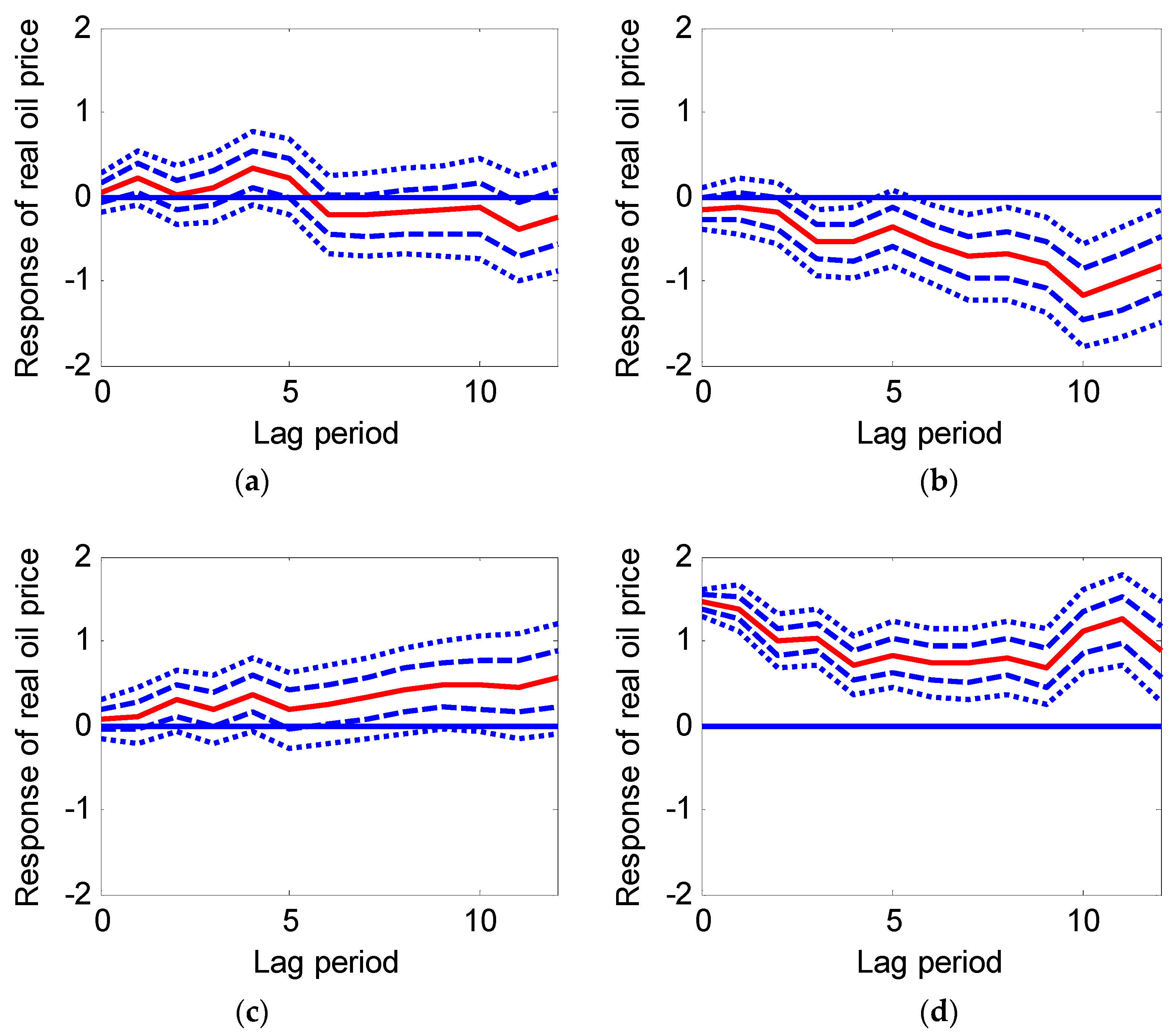
Figure 3 displays the responses of real oil price to one standard deviation structural innovations in (1) oil production, (2) natural gas production, (3) economic activity, and (4) oil market specific factors, respectively. First, unanticipated increase in oil supply just has only a small and statistically insignificant effect on the real price of oil, which is consistent with Kilian [8]. This might be explained by the fact that oil supply increase in one region usually lead to endogenous oil production shrink in other regions which tend to offset the initial production expansion. Second, economic activity expansion also causes a persistent and significant increase in the real oil price. Much of this effect is delayed by half a year which is consistent with that in Dudian et al. [41], and the effect does not decline even after 12 months. Third, oil market specific shocks, such as unanticipated precautionary demand increase, would immediately and persistently drive up the real price of oil. The result is consistent with Alquist and Kilian [42] which provide a theoretical model to show how specific shocks in the oil market causes precautionary demand increase, resulting in an immediate increase in real oil price.

As for the objective of this paper, perhaps the most interesting result in Figure 3 is the fact that natural gas production expansion has a gradually increasing and persistent negative effect on real oil price. It starts to decline only after 10 months. There is some implication that the increase in natural gas production caused by shale gas revolution might subsequently drag down real oil price. Since factor inputs are fixed in the short run and the substitution process from oil to gas are time-consuming, we expect the changes in natural gas production to have a lagged effect on real oil price.

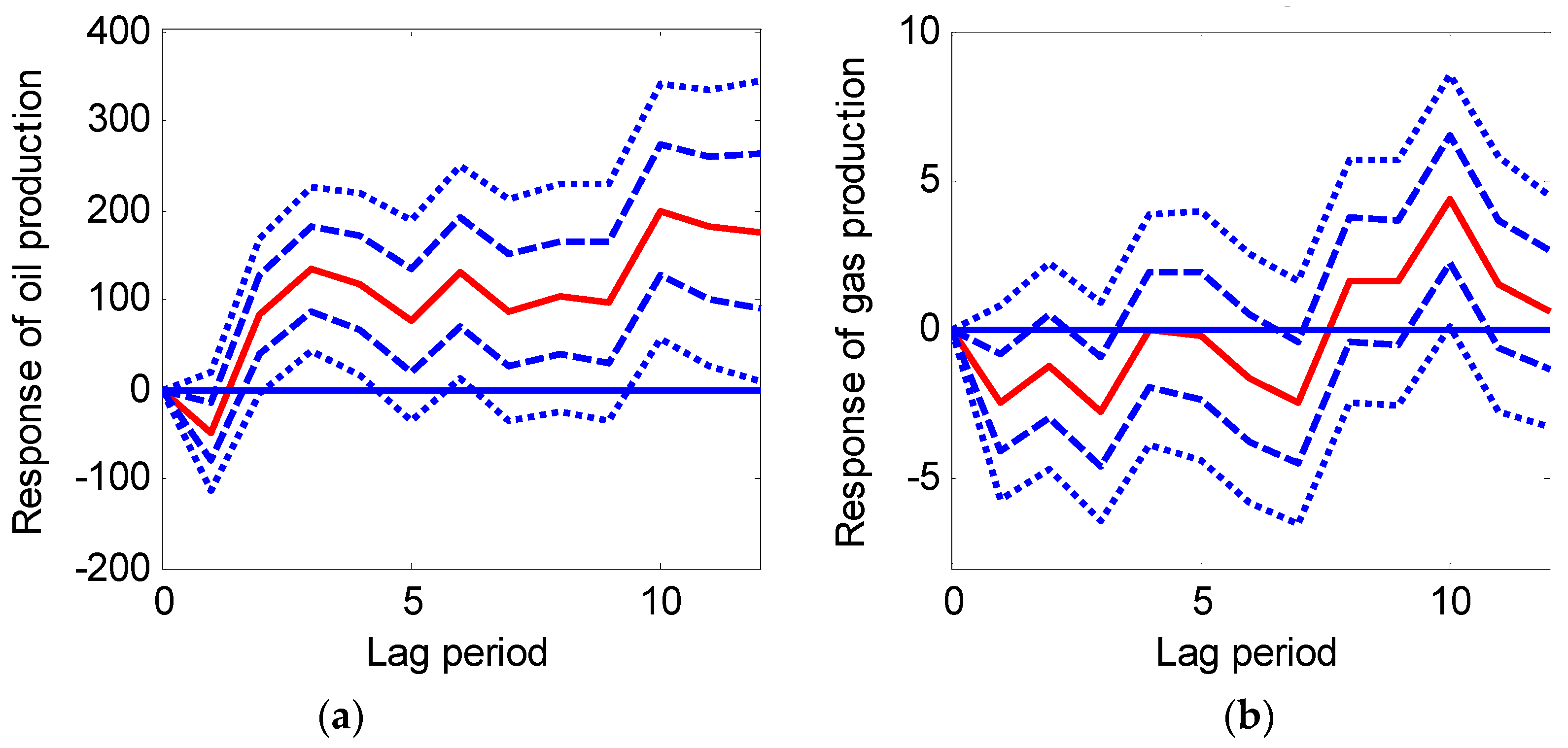
It is worth noting that the SVAR specification in Equation (4) does not indicate that crude oil and natural gas productions are not affected by crude oil price, but that they respond to oil price shocks with a delay of at least a month. This assumption is reasonable given the costs of adjusting oil and natural gas production and the time-consuming adjustment process. Figure 4 shows the responses of oil and natural gas production to oil price increase. The magnitude of vertical axis is different because the units of production for crude oil and natural gas vary considerably, and thus they have different orders of magnitude. The mean for oil production is 80,543 thousand barrels per day, while the mean for natural gas production is 2094 billion cubic feet.

A positive shock in oil price causes a persistent and significant increase in crude oil production with a delay of 2 months, as shown in Figure 4a. This pattern is consistent with supply curve and easy to understand. The more striking result in Figure 4b is that crude oil price shocks do not have significant effect on natural gas production, which could be explained by the fact that natural gas and crude oil are complements and rivals in production. Geologically, there are two forms of natural gas: associated gas which is found in oil fields, and non-associated gas which is isolated in natural gas fields. According to Villar and Joutz [43], about 14% of total natural gas production comes from associated gas, which is usually extracted from oil fields. In this regard, the productions of natural gas and oil are complementary. Meanwhile, the remaining 86% of natural gas is non-associated. The miners of natural gas need to compete for similar factor inputs with crude oil operators, such as drilling rigs and skilled labors. For example, an increase in oil production would induce more demand for these factor inputs, and hence result in higher costs of relevant factors, leading to an increase the cost of mining natural gas. Therefore, natural gas and oil are rivals in production as well.

The response of natural gas production presented in Figure 4 is now plausible. Oil production increase caused by positive oil price shocks lead to increase in associated gas production due to the increase in crude oil production (as shown in Figure 4a), but the production of non-associated gas might be reduced due to the rivalry from crude oil. The mixed response of natural gas production is thus ambiguous (as shown in Figure 4b).

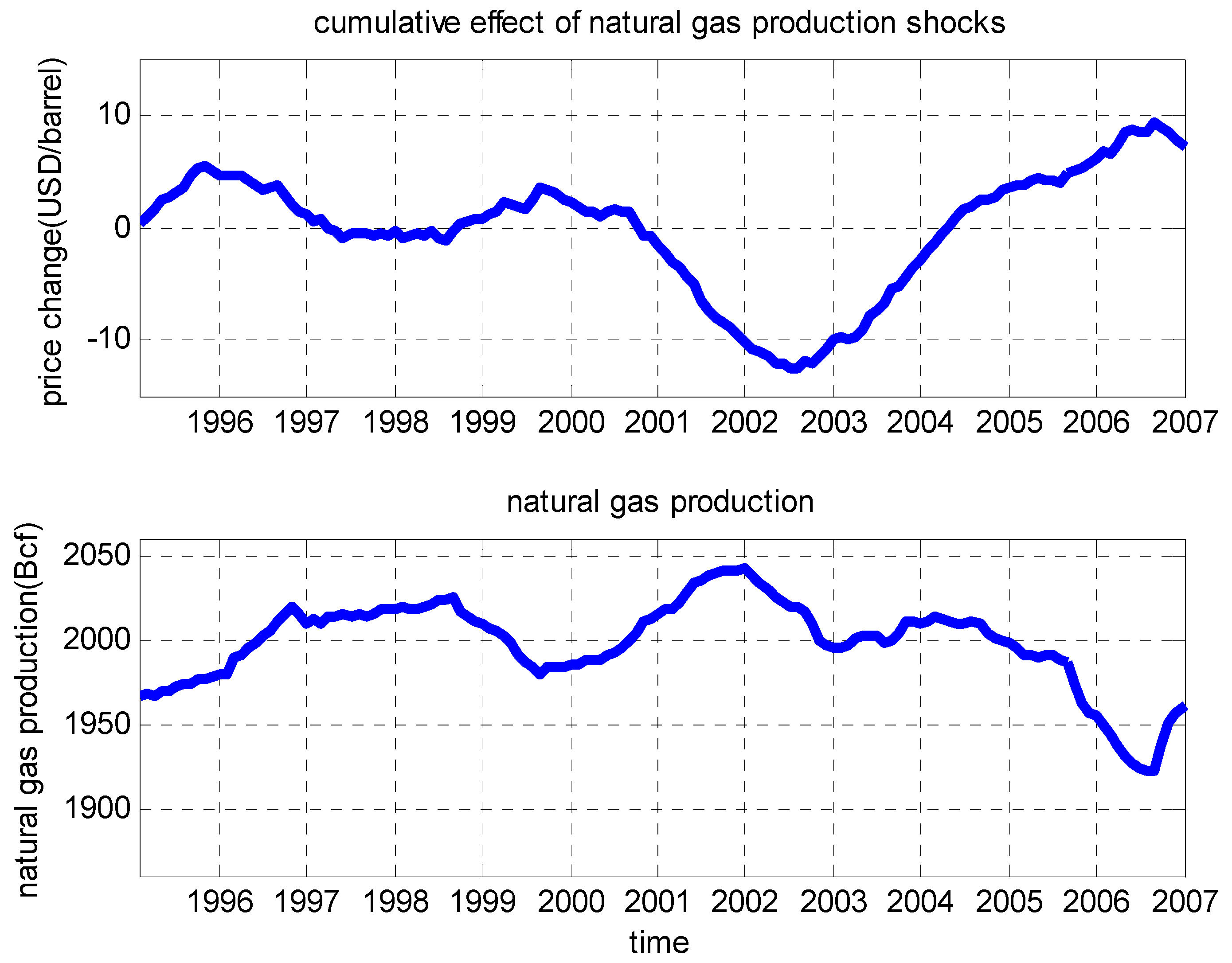
The evolution of real oil price is driven by the four factors in the structural VAR model. We particularly identify the cumulative contribution of natural gas production as shown in Figure 5. For comparison, the natural gas production is also displayed correspondingly. The results show that changes in natural gas production is indeed partly responsible for the increases and decreases in the real oil price. Several important features are apparent in Figure 5.

(i)

The cumulative impact of natural gas production on real oil price is highly negatively correlated with the production of natural gas, indicating that production expansion of natural gas caused by shale gas revolution might have large negative effect on real oil price.

(ii)

Changes in real oil price in response to the shocks in natural gas production is delayed by several months. This is consistent with the results of persistent impulse response presented in Figure 3b. For example, the largest negative contribution to real oil price happened in July 2002, as predicted by the largest expansion of natural gas supply in December 2001. This implies that the contribution of shale gas revolution to real oil price might also be somewhat delayed.

(iii)

Before shale gas boom, the contribution of natural gas production to real oil price is either positive or negative depending on increase or decrease in natural gas production. Natural gas production shocks have little systematic predictive power on changes in the real oil price. On average, changes in natural gas production just have a small effect on the real oil price (−0.16 USD/barrel). However, as analyzed in Section 5, due to continuous expansion of natural gas production, shale gas revolution tends to trigger a dramatic and persistent decrease in the real price of oil.

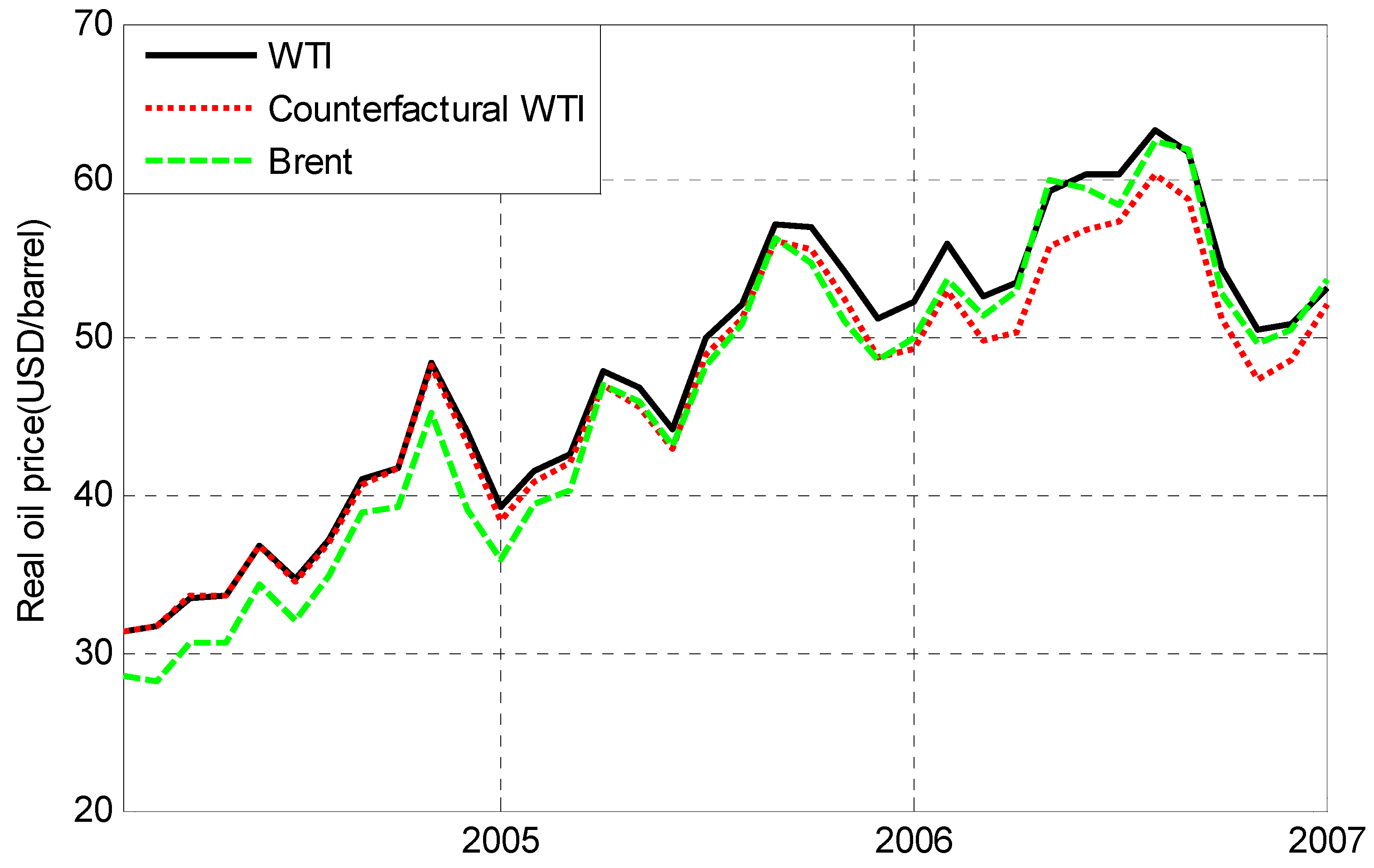
Figure 6 displays the historical evolution of WTI real oil price and its counterfactual in the absence of shale gas revolution. For comparison, the Brent real oil price is also presented. The trend of WTI price and its counterfactual behave similarly until 2009. On one hand, the production expansion of shale gas gradually and steadily increased after 2007. In 2007, the proportion of shale gas in US total natural gas production was 5.2%, while shale gas became a large scale phenomenon in 2009, accounting for 12.0% in total US natural gas supply. On the other hand, this fact is consistent with the view that the cumulative contribution of shale gas expansion to real oil price is delayed (as shown in Figure 5) due to the gradually increasing and persistent impulse response (as shown in Figure 3). From 2009, with the expansion of shale gas and delayed cumulative contribution of shale gas shocks, the actual and counterfactual real oil price diverge obviously, and the gap seems to increase.

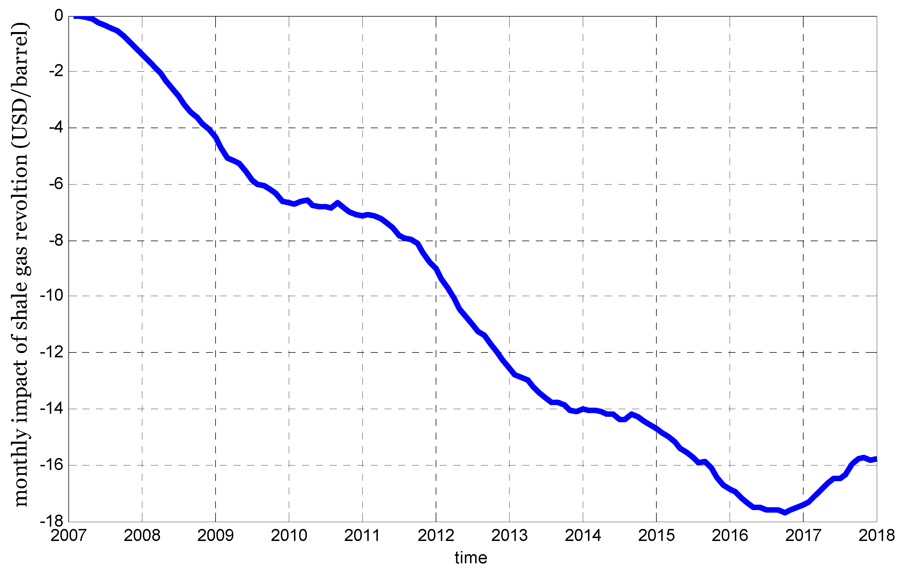
The discrepancy between actual and counterfactual lines in Figure 6 reveals a large negative impact of shale gas expansion on real oil price. Figure 7 further depicts the monthly estimates of the impacts of shale gas revolution, that is, the monthly gaps in real oil price between the actual series and counterfactuals. Figure 7 suggests that shale gas revolution had a substantial effect on real WTI oil price, and that the effect increased with time. In general, the WTI real oil price is 18 percent lower than those of the counterfactuals. The gap in real oil price would increase during the sample period, taking values around 46% in 2017.

It is instructive to compare the counterfactual WTI oil price with Brent oil price which appears to be little affected by US shale gas expansion. Before shale gas revolution, real WTI oil price generally has a premium to Brent price by an average of 1.66 USD/barrel, but the premium is reversed after shale gas boom. For the period from 2007 to 2013, the actual WTI price is on average 4.50 USD/barrel lower than Brent price. At least part of this reversal is likely to be explained by the influence of shale gas revolution. Our results suggest that for the 2007–2013 period, real WTI oil price was reduced by an average of 6.93 USD/barrel while before shale gas revolution it was only −0.16 USD/barrel, as displayed in

Table 2. The impact of shale gas revolution on real WTI price (USD/barrel).

	Before Shale Gas Revolution 1994–2006 (1)	After Shale Gas Revolution 2007–2013 (2)	After Shale Gas Revolution 2014–2017 (3)
Magnitude of impact	−0.16	−6.93	−15.98
Gap between WTI and Brent oil price	1.66	−4.50	−2.38

. In the absence of shale gas revolution, the gap between counterfactual WTI and Brent price would be 2.43 (2.43 = −4.50 − (−6.93)) USD/barrel which was only slightly larger than the value before 2007. During 2014–2017, the impact of shale gas revolution on oil price was even larger because of the ever-increased shale gas production. Compared with the counterfactuals without shale gas intervention, WTI oil price has been decreased by 15.98 USD/barrel. Yet, different from the period 2007–2013, the gap between WTI and Brent oil prices narrowed to be 2.38 USD/barrel which is much smaller than the shale gas impact (15.98 USD/barrel). An explanation is that, in recent years, many new pipeline takeaway capacity has been built at Cushing which is the hub of US oil trade [34], enabling crude oil to flow to and from the trading hub more easily. Thus, the downward pressure on the price of WTI can be transmitted to the price of Brent oil, narrowing the gap between WTI and Brent oil prices.

5. Further Discussion: The Placebo Study

The question that remains to be answered is whether the gap between actual WTI oil price and counterfactuals depicts in Figure 5 truly responds to the impulse of shale gas revolution, or is it merely an artifact of the inability of our analysis to reproduce the evolution of real WTI price without the intervention of shale gas expansion. In order to answer this question, a “placebo study” is performed by employing the method of constructing counterfactual real WTI price to a “no shale gas period” (a period before shale gas revolution which the production of shale gas is small).

The idea is to analyze the evolution of real oil price if we had chosen a period at random without shale gas expansion instead of 2007–2017. The purpose is to evaluate whether the price gap observed for the real WTI oil price may have been driven by chance, other than shale gas revolution. If the placebo study also reproduces gaps between the actual and the counterfactual real WTI oil price before the shale gas revolution, the interpretation is that our results do not provide significant evidence of a negative price effect of shale gas revolution. If on the other hand, the placebo study demonstrates that the gap estimated for the period after shale gas revolution (2007–2017) is unusually large relative to the gap estimated before the shale gas boom, the interpretation is that our results do provide significant evidence of a negative effect of shale gas revolution on real WTI oil price.

To conduct this placebo study, we chose the period 2004–2006 when shale gas production is still very small (2~3% on average) and might not create substantial impacts on oil price. Similarly, sample period 1994–2003 is used for identifying the relations between natural gas production and real WTI oil price, and then the identified relations is applied to construct the counterfactuals of real WTI oil price between 2004–2006.

Figure 8 shows the results of the placebo study. Our results provide an excellent fit for real WTI oil price prior to shale gas expansion. The counterfactuals extracting the influence of shale gas could reproduce real WTI oil price with high accuracy in the period 2004–2006. Considering that the production of shale gas in 2004–2006 only accounted for 2–3% of total US natural gas production, the result is quite convincing. Therefore, as the placebo study indicates, real WTI oil price can be reasonably well reproduced by our models, the estimated gap for real WTI price during 2007–2017 is unusually large relative to the period before the shale gas revolution, and thus the large price effect could be attributed to shale gas revolution.

6. Conclusions and Policy Implications

Since the mid-2000s, especially 2007, shale gas has become an important energy type that has transformed the global energy landscape. Since natural gas and oil are substitutes in consumption, as well as complements and rivals in production, natural gas and oil are linked through both supply and demand sides. The expansion of shale gas production, commonly referred to as “shale gas revolution”, might create substantial impact on oil price. Much has been discussed regarding the impact of the shale gas revolution on the energy market, however to date, little research has been conducted to quantitatively evaluate this issue. This paper fills the research gap by providing empirical evidence of a substantial negative effect of the shale gas revolution on real WTI oil price.

The first part of this study identifies the effect of natural gas production on real oil price by applying structural VAR model. Then we construct the counterfactuals of oil price without shale gas revolution based on the results of the identification. Finally, the magnitude of shale gas revolution on real oil price could be assessed using the gap between actual and counterfactual series.

This paper demonstrates that the expansion of natural gas production has a gradually increasing and persistent negative effect on real oil price, indicating that production expansion of natural gas caused by shale gas revolution might have large negative effect on real oil price. The counterfactual analysis provides evidence that shale gas revolution from 2007 to 2017 has reduced real WTI oil price by an average of 10.22 USD/barrel, which accounts for 18 percent of real WTI price.

We further address the question of whether our results might be caused entirely by chance. A placebo study is therefore performed, which support the hypothesis that the counterfactuals of real WTI oil price can be reasonably well reproduced by our models and the estimated gap for real WTI price during 2007–2017 can be attributed to shale gas revolution.

Global oil demand is growing strongly, particularly in China and India. Furthermore, it is highly likely that oil demand in emerging markets will continue to grow at a remarkable rate [44]. With stagnated oil supply, the rise in oil price in the long run seems to be inevitable [45]. Measures such as improving energy efficiency, investing in renewable energy, are usually regarded as pathways for reducing the unbalance between oil demand and oil supply [46]. The empirical study conducted in this paper provides some evidence that the expansion of shale gas production is an alternative choice for mitigating the increase in oil price.

Finally, it is worth noting that although this paper focuses on the shale gas revolution, the methodology and framework employed in the article can be applied to evaluate the economic impacts of other programs or policies.