Can Energy Structure Optimization, Industrial Structure Changes, Technological Improvements, and Central and Local Governance Effectively Reduce Atmospheric Pollution in the Beijing–Tianjin–Hebei Area in China?

Abstract

Economic growth in the Beijing–Tianjin–Hebei region has been achieved by consuming large amounts of fossil fuels. This produces a large number of pollutants, which damage the physical and mental health of residents, and prevent sustainable economic development. The most urgent task at present is improving the quality of the environment. This paper takes carbon emission as a pollution index, and adopts an extended stochastic impacts by regression on population, affluence, and technology (STIRPAT) model in order to study the impact of the optimization of industry structure (in particular the reduction of the proportion of energy-intensive secondary industry), the optimization of the energy structure, and technological improvements on the atmospheric environmental quality. We obtain some important and enlightening discoveries. First of all, the rapid economic growth that has been based on magnanimous fossil fuel consumption is still the main reason for the deterioration of the atmospheric environment. This means that the main driving force of economic growth still comes from high pollution industries, despite a strategy for the transformation of the pattern of economic growth having been proposed for many years. Second, the optimization of the industrial structure has not played a significant role in promoting the reduction of carbon emissions. Through further research, we believe that this may be due to the low-quality development of the third industry. In other words, the traditional service industry related to high energy consumption accounts for a large proportion in regional total output, while the high-end service industry related to small pollution accounts for a relatively small proportion. Third, reducing the consumption of coal and improving the technological level can effectively curb the deterioration of the environmental quality. In addition, we find that transboundary pollution is an important factor affecting the environment in this region, and the earnings of any unilateral treatment action is small. As a result, joint pollution control under the supervision of the central government can produce greater benefits. Therefore, we believe that the transition of the economic growth pattern, and the optimization of the energy and industry structures (especially developing the high-end service industry) are effective ways to improve the environmental quality.

1. Introduction

China’s economy has maintained rapid development more than 30 years after the reform and opening-up policy. In 2010, China surpassed Japan and became the second largest economy in the world. Although the extensive mode of development has led to rapid economic growth, it has also caused serious damage to natural resources and the ecological environment. In recent years, the continuous extreme haze weather across the country has seriously affected the people’s physical and mental health. As a major heavy industry base in China, the Beijing–Tianjin–Hebei area and its surrounding areas have many high-pollution industries such as steel, chemicals, cement, etc. The world’s urban air quality data, which was published by World Health Organization (WHO) in May 2017, showed that the Beijing–Tianjin–Hebei region occupies the top nine positions among cities with the highest density PM_2.5 in China: Xingtai, Baoding, Shijiazhuang, Handan, Hengshui, Tangshan, Langfang, Cangzhou, and Tianjin. Beijing is not in the top 10; it ranks 11th. Cases of such serious and centralized pollution are very rare. Related research studies have shown that serious particulate pollution is closely related to human genome variations, respiratory diseases, and cardiovascular diseases [1,2,3,4]. Furthermore, environmental pollution also has an adverse influence on the sustainable development of the economy, since the development of the regional economy must consume certain environmental resources, which refers to the exploitation of natural resources and the emission of pollutants. However, there is an upper limit regarding the ecological environment’s ability to hold the pollutants produced by human productive activities. Once the discharged pollutants exceed the quantity that the natural environment can purify by itself, it will cause enormous damage to the ecological environment, and the sustainable development of the economy cannot be achieved. National atmospheric environmental-bearing capacity research based on new air quality standards have shown that 70% of 330 prefecture-level cities in China have overloaded atmospheric environments, and the most serious overloaded areas include the Beijing–Tianjin–Hebei region and its surrounding areas [5]. Therefore, some actions to improve the quality of the atmospheric environment are urgently needed.

Energy-related pollutant emissions are the main causes of environmental pollution in the Beijing–Tianjin–Hebei region. The energy consumed is mainly fossil fuels such as coal, petroleum, and natural gas, accounting for more than 98% of the total energy consumption, and the proportion of renewable, non-polluting energy accounts for a small proportion, which cannot be fundamentally changed in the short term. Although experts and scholars in relevant fields all recognize that energy-related pollutant emissions are the major environmental pollution in the region, they do not know how to reduce pollutant emissions while ensuring economic growth. For example, since we all know that the tertiary industry consumes less energy than the secondary industry, is the rapid increase in the tertiary industry’s share of the economy the most effective way to reduce pollutant emissions? Moreover, natural gas combustion produces fewer pollutants than coal; so, can the reduction of coal and an increase in the production of natural gas effectively reduce pollutant emissions? What’s more, we know that the improvement of technology can reduce energy consumption, but that there is also a trend of decreasing margins. To what extent is the region’s economy technological, and can the improvement of it significantly reduce the emission of pollutants? Most importantly, the strategy of transforming the economic growth mode has been implemented for many years; has the regional economic growth strategy already gotten rid of the situation of high-energy consumption and high pollution? The solutions to these problems can help us better understand which policies are the most effective in reducing pollutant emissions.

Transboundary pollution is an important factor in the deterioration of the air quality in the Beijing–Tianjin–Hebei region. Atmospheric pollution can easily cross the border between regions, which is different from other types of environmental pollution. On the basis of the third generation WRF-CAMx (Weather Research Forecast-Comprehensive Air Quality Model Extensions) model, China’s Environmental Protection Planning Institute simulated transboundary transport rules of PM_2.5 among each province across the country. The research shows that 34% of the PM_2.5 particulate pollutants in Beijing come from other provinces, of which 22% come from Hebei and Tianjin. Meanwhile, the transboundary transport rate of Tianjin is 44%, including 23% from Hebei and Beijing. The data comes from China’s Environment Planning Bureau within the Environment Protection Department. Under the “territorialism” of administration, the existence of transboundary pollution has increased the difficulty of air pollution control. Local governments tend to focus on rapid economic growth, while little attention is paid to the impact of pollution on the surrounding environment, which often leads to underestimating the cost of environment treatment. The regional atmospheric environment is a kind of public resource, which is non-competitive and non-exclusive; as a result, excessive consumption inevitably leads to the “tragedy of the commons”, which results in the deterioration of the overall environmental quality in the region. Therefore, joint control among the regional governments is an inevitable choice. However, it is hard to avoid the existence of “free riding” in the process of joint governance, where the local government has no incentive to actively control pollution, and the prisoners’ dilemma exists. The ability to promote effective cooperation among local governments can greatly enhance the benefits of pollution control. In this paper, we find that the strict supervision of the central government on pollution control by local governments can effectively prevent the prisoners’ dilemma.

Although human activities have caused serious damage to the ecological environment, people can’t understand the driving forces behind it scientifically in the early stages. A very important reason is the lack of a scientific model that explores the relationship between human activities and environmental change. The earliest model used for studying the relationship between human activities and the natural environment is the IPAT (Namely I=PAT. It is the mathematical notation of a formula put forward to describe the impact of human activity on the environment model. The expression equates human impact on the environment to the product of three factors: Population, Affluence, and Technology) model. As a logical framework, the IPAT model is widely used to study the impact of human activities on the natural environment [6,7]. However, the model has serious limitations in practical application. For example, the influencing factors in the model all change linearly with proportionality, and the hypothesis test is not allowed. In order to overcome those defects, the STIRPAT model emerged [8]. The STIRPAT model is a regression model that involves the random influence of population, affluence, and technology on the environment, and has been successfully applied to analyses of the influence of human activities on the environment [9,10,11,12]. So, the extended STIRPAT model will be applied in this article.

Most of scholars who study atmospheric environmental pollution of China always select regional industrial waste gas (i.e., sulfur dioxide), oxynitride, and smoke (dust) to be the index of environmental pollution measurement. Since carbon compounds are important parts of particulate pollutants, and the greenhouse gas effect caused by carbon emissions has become an urgent problem to be solved in various countries in recent years, we take carbon emissions to be the index of environmental pollution in the Beijing–Tianjin–Hebei region in order to test the pollution levels of the environment. Considering the complexity of factors that affect carbon emissions, many scholars tend to expand the STIRPAT model according to the actual conditions in the countries or regions studied. Abdallh et al. [13] used the panel data of 20 countries in the MENA (Middle East and North Africa) area to study the relationship between urbanization levels and carbon emissions. It turns out that continuous urbanization can reduce the number of carbon emissions per capita, but the most significant contributor to carbon emissions is energy consumption and economic growth. In the future, countries that are committed to reducing carbon emissions should focus on economic growth rather than urbanization. Liu et al. [14] hold a different opinion than Abdallh. They believe that an improvement in urbanization levels will promote the increase of carbon emissions, and a low-carbon economy development path is the most important way to realize carbon emission reduction. Shahbaz et al. [15] focused on observing the influence of urbanization on carbon emissions in Malaysia, finding a U-type relationship between urbanization levels and carbon emissions. That is to say that the initial phase of urbanization can restrain carbon emissions, but it will also promote the increase of carbon emissions after exceeding a certain threshold value. Zheng et al. [16] applied the panel data of 73 cities in China in order to study the influence of the population size, industrial structure, energy structure, urbanization level, and economic development level on carbon emissions at the city level. The result shows that these factors have a positive influence on carbon emission, but the urbanization level is not prominent in statistics. Wen et al. [17] studied the influencing factors of China’s energy production on carbon emissions, and found that size and industrial structure have the largest influence on carbon emissions, followed by energy consumption structures, urbanization levels, and per capita real GDP (Gross Domestic Product). The degree of foreign trade and the technological level have the least impact on carbon emissions. They think that controlling population growth and optimizing the industrial structure are effective ways of reducing carbon emissions. Wang et al. [18] conducted an empirical analysis on the data of Guangdong Province, China, and found that the population size, actual GDP per capita, and industrialization level all have a positive influence on carbon emissions. The improvement of the technological level, the optimization of the energy structure, and an increase in foreign trade can all reduce carbon emissions. They also found that the population size is the most important factor influencing carbon emissions, while the influences of the technological level and foreign trade are limited. Lin et al. [19] used China’s data from 1978 to 2006 to conduct an empirical analysis on the factors influencing carbon emissions. The results showed that the influences of the population size, urbanization levels, actual GDP per capita, industrial structure, and technological levels on carbon emission reduce, one after another. They also think that the strict one-child policy of China has also played a very important role in restraining the increase of carbon emissions. Carbon-emission controlling in the future depends on whether people will form low-carbon and environmental-friendly living habits. O’Neil et al. [20] mainly observed the influences of changes of population factors (including population size, aging, urbanization, and family size) on carbon emissions. Their empirical analysis of historical trends showed that the carbon emissions of energy use were nearly in direct proportion to changes in the population size. The influences of aging and urbanization on carbon emissions were relatively small, but they were prominent in the statistics. Beside this, the scenario analysis showed that different population growth paths had substantial influences on carbon emissions over future decades. Liddle [21] used national-level data to study the influences of income and population size on carbon emissions. The result showed that the carbon emission elasticity of income was highly steady, but the carbon emission elasticity of income of an OECD (Organization for Economic Co-operation and Development) country was smaller than that of a non-OECD country. Being different from this, the carbon emission coefficient of population size is not steady, no matter whether it is an OECD country or a non-OECD country, and it is not prominent in statistics. The study of Fan et al. [22] showed that population size, affluence, and the technological level of different development levels all have obvious and different influences on carbon emission.

Through combing the literature, we found that the degree of importance that was assigned to each factor varied greatly by region. In particular, past research showed that the impact of changes in industrial structures on carbon emissions varied greatly by region. So, the purpose of this paper is to solve the following problems. What is the most important factor affecting the carbon emissions in the Beijing–Tianjin–Hebei region? Can a large-scale natural gas coal substitution strategy in the region effectively reduce pollutant emissions? Can the continuous optimization of the industrial structure of the whole area under the coordinated development strategy of the region considerably improve the regional environmental quality? Besides, previous studies didn’t deal with transboundary pollution. The cross-boundary air pollution in the region is very serious. The “externality” of environmental pollution and the unavoidable “hitchhiking” during the process of treatment have become the most important impediments to the improvement of air quality. How can local governments be encouraged to actively participate in the treatment of environmental pollution and avoid the “prisoners’ dilemma”? Solving these problems will greatly help improve the area’s air quality.

The following content of this article is arranged as follows. Part 2 is about variables, models, and data; here, we mainly explain why variables are important, and provide the definition of variables and the specific extended STIRPAT model. We also provide the basic characteristics of the data, and a detailed description of the data source. Part 3 includes the empirical results and analysis; Here, we performed a multiple linear regression on the explanatory and explanatory variables. In order to ensure the validity of the parameter estimation, we also tested and removed the variables that caused multicollinearity, and eliminated the autocorrelation of the residual sequences. All of the work improved the accuracy of the model parameters. Part 4 is about the game between local governments. We find that there is a prisoners’ dilemma in the joint control of environmental pollution by local governments, and we think that strict supervision of local governments by the central government can ensure their active participation in pollution control. Part 5 includes the conclusions and policy suggestions. Based on the estimations, the paper provides practical and effective policy recommendations for reducing carbon emissions in the region.

2. Variable, Model, Data

2.1. Variable

Based on the references in the previous literature, and taking into account the actual situation of the Beijing–Tianjin–Hebei region and the availability of relevant data, this paper selects energy carbon emissions as the explained variable measuring the environmental pollution degree, and adds the industry structure, energy structure, and urbanization level to the STIRPAT model in order to form an extended STIRPAT model. The definition of the variable symbol and the specific meaning of the variables are shown in

Table 1. Variable name and definition.

Variable	Symbol	Definition
Carbon emission	I	Total carbon emissions of energy consumption.
Population	P	Total number of permanent residents in the region.
Affluence	A	Actual GDP per capita in the region.
Technical level	T	Consumption of standard coal per 10,000 Yuan of GDP.
Urbanization level	C	Percentage of urban population in the total population.
Energy structure	N	Proportion of coal in total energy consumption.
Industrial structure	S	Proportion of the second industry in regional GDP.

. The addition of these variables will give us a deeper understanding of the causes of air pollution. This is far more meaningful than a model that is built solely on pollutant emissions and energy consumption, or the STIRPAT model alone. For example, in recent years, China’s industrial structure has undergone tremendous changes. It shows that the tertiary industry has rapidly increased its share of GDP, and contributed more to the economy than the secondary industry, making it the industry that has made the largest contribution to economic growth. Therefore, we wonder how changes to the industrial structure will impact energy carbon emissions. In addition, in order to reduce pollutant emissions, the region has implemented a large-scale natural gas coal replacement strategy, which has led to a rise in the price of natural gas in the international market. We wonder whether the implementation of this measure will have a positive effect on air quality improvement, and if so, whether the effect is significant. The extended STIRPAT adopted in this paper can provide a scientific answer to these questions, as well as provide a scientifically valid reference for pollution control by the government.

2.2. Model

The STIRPAT model is one of the most successful models for studying the impact of human activities on the environment, and can be expressed by the following equation:

$$I_t={\alpha }_0{P_t}^{{\alpha }_1}{A_t}^{{\alpha }_2}{T_t}^{{\alpha }_3}{\epsilon }_t$$

(1)

Among them, the meanings of I, P, A, and T are the same as that in the IPAT equation. α_i (i = 0, 1, 2, and 3) are the estimated parameters. ε_t is a random disturbance term measuring the impact of unobserved factors on carbon emissions. The extended STIRPAT model used in this paper can be expressed as follows:

$$I_t={\alpha }_0{P_t}^{{\alpha }_1}{A_t}^{{\alpha }_2}{T_t}^{{\alpha }_3}{C_t}^{{\alpha }_4}{N_t}^{{\alpha }_5}{S_t}^{{\alpha }_6}{\epsilon }_t$$

(2)

Take the logarithm of both sides of Equation (2):

$$\ln I_t=\ln {\alpha }_0+{\alpha }_1\ln P_t+{\alpha }_2\ln A_t+{\alpha }_3\ln T_t+{\alpha }_4\ln C_t+{\alpha }_5\ln N_t+{\alpha }_6\ln S_t+\ln {\epsilon }_t$$

(3)

Among them, I, P, A, and T have the same meaning as in Formula (1), and the added variables C, N, and S are urbanization level, energy structure, and industrial structure respectively. The specific definition of variables refer to Table 1.

2.3. Data

The data in this paper are compiled from the Beijing Statistical Yearbook, the Tianjin Statistical Yearbook, and the Hebei Economic Yearbook. Pollutant emissions are based on the region’s carbon emissions. Since fossil fuel combustion is the main source of carbon emissions, this paper uses the carbon emissions from energy consumption as a statistical indicator. There are many ways to estimate energy-related carbon emissions. This article refers to Guo [23], and only calculates the combustion emissions of major energy sources, including coal, oil, and natural gas. Taking into account the differences in the carbon emission factors for each energy type, the following formula is used to calculate the total amount of carbon emissions:

$$I={\displaystyle \sum _{i=1}^{i=3}{H}_i}{K}_i(i=1,2,3)$$

(4)

where I represents total carbon emissions, and i = 1, 2, 3 represent the three energy sources of coal, oil, and natural gas, respectively. H_i represents the consumption amount of energy, i. K_i represents the carbon emission coefficient of energy, i. The institutions in different countries have different evaluation values for carbon emission coefficients. We refer to Wu [24], making calculations by the average value of the data, which is announced by six institutions, such as DOE/EIA (DOE is U.S. Department of Energy and EIA is U.S. Energy information Administration), the Japan Energy Economics Institute, the National Development and Reform Commission Energy Research Institute, etc. Detailed information is shown in

Table 2. Carbon emission coefficient of main energies.

Research Institute	Coal	Petroleum	Natural Gas
DOE/EIA	0.7020	0.4780	0.3890
Japanese Institute of Energy Economics	0.7560	0.5860	0.4490
Energy Research Institute of National Development and Reform Commission	0.7476	0.5825	0.4435
Chinese Academy of Engineering	0.6800	0.5400	0.4100
Greenhouse gas control project of the National Environment Protection Agency	0.7480	0.5830	0.4440
Climate change project of the State Scientificand Technological Commission	0.7260	0.5830	0.4090
Average value	0.7266	0.5588	0.4221

. The GDP indices involved are all calculated at constant prices, with a base period of 2005.

Table 3. Total energy consumption in each region, and the proportion of three types of energy consumption (coal, oil, and natural gas).

Area	Beijing				Tianjin				Hebei
Category	D	E (%)	F (%)	G (%)	D	E (%)	F (%)	G (%)	D	E (%)	F (%)	G (%)
2005	4555	54.38	44.65	0.97	4892	60.28	39.54	0.18	19,703	92.44	7.50	0.06
2006	4685	52.31	46.74	0.95	5118	60.72	39.02	0.26	21,641	92.24	7.69	0.07
2007	4998	48.00	51.12	0.88	5376	61.06	38.61	0.33	23,420	93.01	6.92	0.07
2008	5068	41.67	56.59	1.74	5286	63.38	36.20	0.42	24,097	93.01	6.92	0.07
2009	5225	39.42	58.89	1.69	5651	63.07	36.54	0.39	25,124	93.17	6.73	0.10
2010	4824	37.46	60.66	1.88	7173	54.49	45.14	0.37	25,645	93.60	6.28	0.12
2011	4683	34.55	63.54	1.91	7607	55.43	44.17	0.40	27,339	91.49	8.34	0.17
2012	4666	33.36	64.25	2.39	7500	58.25	41.23	0.52	27,767	92.05	7.74	0.21
2013	4370	33.01	64.25	2.74	7983	55.78	43.65	0.57	28,516	92.26	7.51	0.23
2014	4492	27.63	69.30	3.07	7617	56.10	43.19	0.71	28,057	92.44	7.29	0.27
2015	4138	20.10	75.64	4.26	7386	52.65	46.31	1.04	27,886	91.23	8.42	0.35

D stands for the total energy consumption measured in standard coal (10,000 tons). E, F, and G represent the proportion of coal, oil, and natural gas in total energy consumption, respectively.

are the total energy consumption in each region, and the proportion of each region’s energy consumption. We do not have statistics on renewable energy, mainly because of its low share of consumption, and the lack of relevant data.

Table 4. Statistical table of carbon emissions and data.

Year	Carbon Emission (Million Tons)	Population (Ten Thousands)	Affluence Degree (Ten Thousands Yuan)	Technical Level (tce)	Urbanization Level (%)	Energy Structure (%)	Industrial Structure (%)
2005	261.9902	9432.00	2.22	1.39	0.4932	0.8132	0.5004
2006	282.7352	9574.00	2.48	1.34	0.5054	0.8001	0.4742
2007	304.0947	9734.00	2.81	1.26	0.5200	0.8007	0.4700
2008	309.4580	9936.00	3.07	1.16	0.5374	0.7873	0.3909
2009	323.1834	10,122.16	3.32	1.11	0.5548	0.7826	0.4764
2010	330.5580	10,454.79	3.69	1.00	0.5663	0.7599	0.5264
2011	348.0558	10,613.69	4.11	0.95	0.5778	0.7499	0.4795
2012	353.2205	10,769.96	4.33	0.91	0.5893	0.7404	0.4961
2013	361.3829	10,919.62	4.53	0.89	0.6008	0.7303	0.4718
2014	353.8921	11,052.16	4.67	0.86	0.6107	0.7163	0.3745
2015	342.8297	11,142.37	4.77	0.84	0.6253	0.6801	0.3201

is the annual data statistics of each variable.

Table 5. Statistical description of variables.

	ln(I)	ln(P)	ln(A)	ln(T)	ln(C)	ln(N)	ln(S)
Average value	10.38	9.24	1.26	0.05	−0.58	−0.28	−0.80
Median	10.41	9.25	1.31	0.00	−0.57	−0.27	−0.75
Max. value	10.50	9.32	1.56	0.33	−0.47	−0.21	−0.64
Min. value	10.17	9.15	0.78	−0.17	−0.71	−0.39	−1.14
Standard deviation	0.10	0.06	0.27	0.18	0.08	0.06	0.15

is the statistical description of each variable.

3. Empirical Results and Analysis

By using the tool eviews8, we made multiple linear regressions by Equation (3) for the data in Table 4. The metering regression results are shown in

Table 6. Model regression result.

Variables	Coefficient	Standard Deviation	T_Value	p_Value
ln(P)	−0.070011	0.639793	−0.109428	0.9181
ln(A)	0.978684	0.081019	12.07961	0.0003
ln(T)	0.666975	0.177858	3.750041	0.0199
ln(C)	−0.044973	0.265163	−0.169606	0.8736
ln(N)	0.594659	0.184596	3.221403	0.0322
ln(S)	0.039635	0.019850	2.001238	0.1160
R2	0.999214	F_value	847.6475
R2 after adjustment	0.998035	P (F_statistic)	0.000004
DW	3.332421	N	11
SSR	8.30 × 10−5

Note: DW is the Durbin Watson statistic, SSR is the sum of residual squares.

.

According to above regression results, the coefficient of determination R² = 0.999214 is very high, which means that factors such as population, affluence, and technological level, etc. could explain 99.9% of the changes in carbon emissions in the Beijing–Tianjin–Hebei region. Meanwhile, the p value of F statistics is 0.000004, which means that the integral significance of regression is high. Although the coefficient of determination is very high, the t values of variable ln(P) and ln(C) are small, and do not pass the significance test under the 5% level. Thus, serious multiple linearity may exist among the explanatory variables. In order to ensure the accuracy of the model, we can remove the variables that were causing multiple linearity. However, removing the variables directly may result in missing important variables. In order to solve the problem, this paper included a linear constraint test to test whether the parameters α₁ = 0 and α₄ = 0 are true. If the restraint is true, it means that the association of these two variables is not significant, and provides the basis for removing them from the model. This paper adopts the likelihood ratio (LR) statistic for inspecting whether the constraint condition is true or not. The original hypothesis (H₀) and alternative hypothesis (H₁) are presented as below:

H₀: α₁ = 0, α₄ = 0;

H₁: H₀ is not true;

Under the original hypothesis condition of a “true constraint condition”, the LR (likelihood ratio) statistic test complies with the χ² distribution of m freedom degree, i.e.:

$$LR~{\chi }_{\alpha }^2(m)$$

(5)

In the equation, m is the quantity of constraint condition, and α represents the significance level. The rule of judgment is as below:

$\mathit{LR}\le {\chi }_{\alpha }^2(m)$, accept the original hypothesis, the constraint condition is true;

$\mathit{LR}>{\chi }_{\alpha }^2(m)$, refuse the original hypothesis, the constraint condition is false.

Based on the regression of the original model, the constrained LR statistic test is carried out. The result is shown in

Table 7. Likelihood Ratio (LR) statistic inspection result.

Statistic	Value	Degree of Freedom	p_Value
LR	0.1046255	2	0.9295

.

According to Table 7, LR = 0.1046255, while on the significance level of α = 0.05, we get ${\chi }_{0.05}^2=5.991$. Thus, we cannot refuse the original hypothesis, i.e., the constraint condition is true. So, we can remove the explanatory variables ln(P_t) and ln(C_t) from the original model, and need not worry about leaving out important variables. Now, we set the model form as below:

$$\ln (I_t)={\alpha }_0+{\alpha }_2\ln (A_t)+{\alpha }_3\ln (T_t)+{\alpha }_5\ln (N_t)+{\alpha }_6\ln (S_t)+u_t$$

(6)

Then, we made a regression in accordance with Equation (6), and obtained the regression result, as shown in

Table 8. Regression results after removing population and urbanization levels.

Variables	Coefficient	Standard Deviation	T_Value	p_Value
ln(A)	0.968275	0.054537	17.75435	0.0000
ln(T)	0.6869891	0.095356	7.204481	0.0004
ln(N)	0.618623	0.105426	5.867812	0.0011
ln(S)	0.040009	0.013596	2.942763	0.0259
R2	0.999204		F_value	1881.997
R2 after adjustment	0.998673		P (F-statistic)	0.000000
DW	3.420013		N	11
SSR	8.41 × 10−5

. After removing the variables causing multiple linearity, all of the explanatory variables went through significance testing under the 5% level. In the meantime, R² after adjustment also increased, which means that the explanatory capability of the model is enhanced.

Although it does not make the estimator lose validity when the residual sequences exist in autocorrelation, the variance is not the smallest, which will decrease the reliability of the model. By adopting the regression inspection method, this paper inspects whether there is an autocorrelation of the random error in the regression equation. Making regression by Equation (7):

$$u_t=\rho u_{t-1}+v_t$$

(7)

In the equation, ν_t satisfies all of the assumption conditions of the multiple linear regression. The regression results are shown in

Table 9. Regression results of Equation (6).

Variable	Coefficient	Standard Deviation	T_Value	p_Value
ρ	−0.762451	0.195357	−3.902869	0.0045

.

According to the Table 9, p = 0.0045, which is far less than the significance level of 5%, i.e., there is a first-order autocorrelation for the residual of the regression in Equation (7). The generalized least square method is adopted to eliminate the autocorrelation. The specific steps are as follows:

(1)

Make Equation (7) into Equation (6), and we get Equation (8):

$$\ln (I_t)={\alpha }_0+{\alpha }_2\ln (A_t)+{\alpha }_3\ln (T_t)+{\alpha }_5\ln (N_t)+{\alpha }_6\ln (S_t)+\rho u_{t-1}+v_t$$

(8)

(2)

Search t − 1 relation to Equation (6), and multiply it by ρ at both sides, and we get Equation (9):

$$\rho \ln (I_t)=\rho {\alpha }_0+\rho {\alpha }_2\ln (A_{t-1})+\rho {\alpha }_3\ln (T_{t-1})+\rho {\alpha }_5\ln (N_{t-1})+\rho {\alpha }_6\ln (S_{t-1})+\rho u_{t-1}$$

(9)

(3)

Subtract both sides of Equations (8) and (9) accordingly, and we get Equation (10):

$$\begin{array}{ll}\ln (I_t)-\rho \ln (I_{t-1})=& {\alpha }_0(1-\rho )+{\alpha }_2\left[\ln (A_t)-\rho \ln (A_{t-1})\right]+{\alpha }_3[\ln (T_t)-\rho \ln (T_{t-1})]\\ & +{\alpha }_5[\ln (N_t)-\rho \ln (N_{t-1})]+{\alpha }_6[\ln (S_t)-\rho \ln (S_{t-1})]+v_t\end{array}$$

(10)

And make:

$$\begin{array}{l}{Y}_t=\ln (I_t)-\rho \ln (I_{t-1})\\ X_{1t}=\ln (A_t)-\rho \ln (A_{t-1})\\ {\mathrm{X}}_{2t}=\ln (T_t)-\rho \ln (T_{t-1})\\ {\mathrm{X}}_{3t}=\ln (N_t)-\rho \ln (N_{t-1})\\ X_{4t}=\ln (S_t)-\rho \ln (S_{t-1})\\ {\beta }_0={\alpha }_0(1-\rho )\end{array}$$

(11)

Then, Equation (10) can be presented by the following form:

$$Y_t={\beta }_0+{\alpha }_2{X}_{1t}+{\alpha }_3{X}_{2t}+{\alpha }_5{X}_{3t}+{\alpha }_6{X}_{4t}+v_t$$

(12)

In Equation (11), ν_t is not an autocorrelation. The parameters obtained by the least square method have an optimal linear without bias when it satisfies the assumption. The regression results are listed in

Table 10. Regression results of Equation (12).

Variables	Coefficient	Standard Deviation	T_Value	p_Value
C	16.48997	0.098363	167.6433	0.0000
X1t	0.957522	0.035570	26.91909	0.0000
X2t	0.665334	0.061060	10.89641	0.0001
X3t	0.650985	0.054470	11.95074	0.0001
X4t	0.038784	0.006260	6.195261	0.0016
R2	0.999917		F value	15136.24
R2 after adjustment	0.999851		P (F-statistic)	0.00000
SSR	1.89 × 10−5		DW	2.911854

.

In order to inspect the autocorrelation of random error in Equation (12), we calculated a regression for the following Equation (13):

$$v_t={\rho }_1{v}_{t-1}+{\hat{v}}_t$$

(13)

According to the regression results in

Table 11. Regression results of Equation (13).

Variable	Coefficient	Standard Deviation	T_Value	p_Value
νt−1	−0.462434	0.314820	−1.468884	0.1801

, p = 0.1801, which is larger than significance level 5%. This means that the residual sequence is not an autocorrelation. At this time, the regression equation is able to reflect the relationship between carbon emissions and each explanatory variable more reliably. According to the conversion relation of Equation (11), we confirm the model as Equation (14), finally:

$$\ln (I_t)=9.35+0.9577\ln (A_t)+0.6653\ln (T_t)+0.6510\ln (N_t)+0.0388\ln (S_t)+u_t$$

(14)

According to the final empirical model, affluence has the greatest impact on carbon emissions. The estimation coefficient of explanatory variable ln(A_t) is 0.9577, which has an economic meaning in that every 1% growth of actual GDP per capita in the region would lead to a 0.9577% growth in carbon emissions. This means that there is a significant and direct positive relationship between economic growth and carbon emissions in the short term, which indicates that the extensive economic growth pattern in the region has not been changed fundamentally. The industry with the highest energy consumption and highest pollution still occupies a large ratio in the economic growth. In the future, in order to ensure medium and-high-speed economic growth, a large amount of energy consumption will be consumed, which will inevitably exert greater pressure on the regional atmospheric environment. At present, the environmental situation in the Beijing–Tianjin–Hebei region is not optimistic. If the atmospheric pollutant emission in the near future is not controlled fundamentally, it may cause catastrophic damage to the ecological environment. It is also difficult to realize sustainable development for the economy. Therefore, all of the localities should actively promote the transformation of the mode of economic growth and develop low-pollution and high-tech industries, which can fundamentally curb the deterioration of air quality.

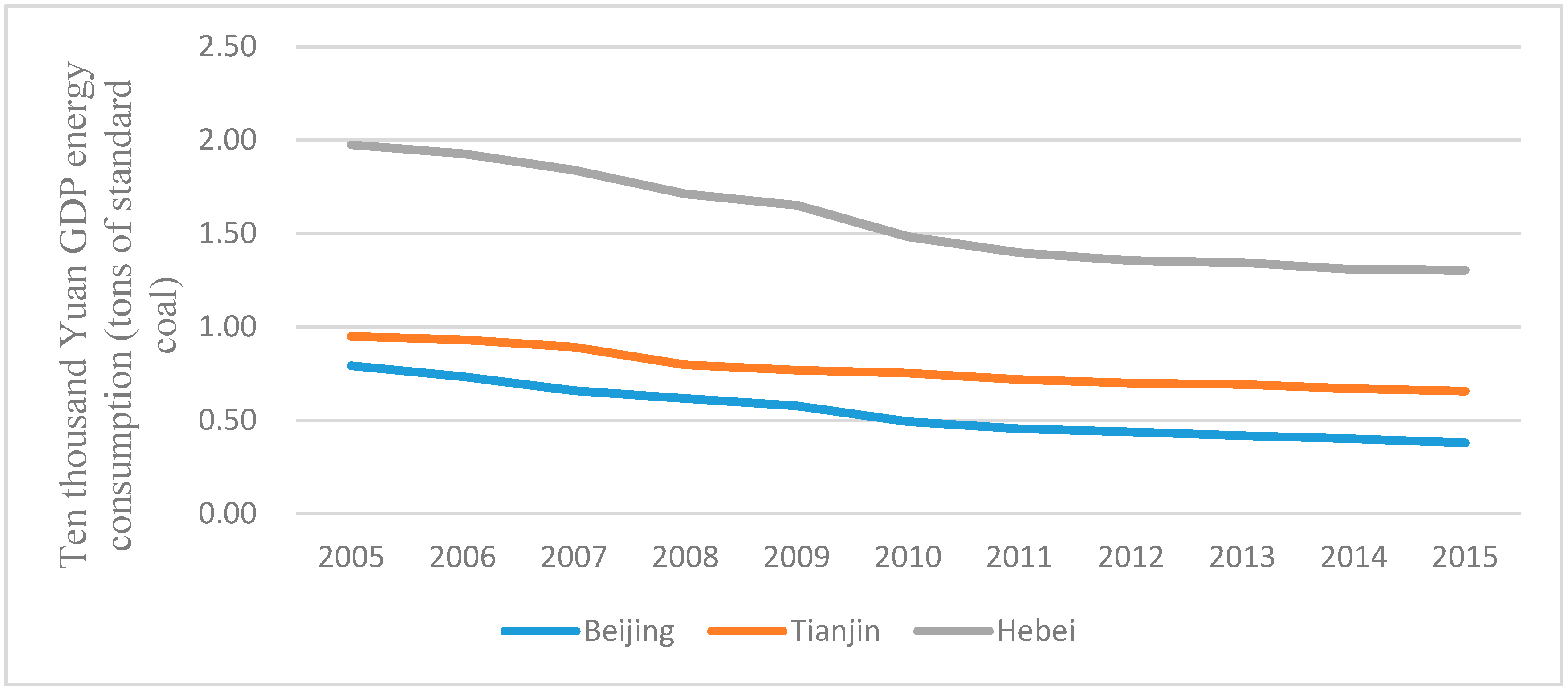
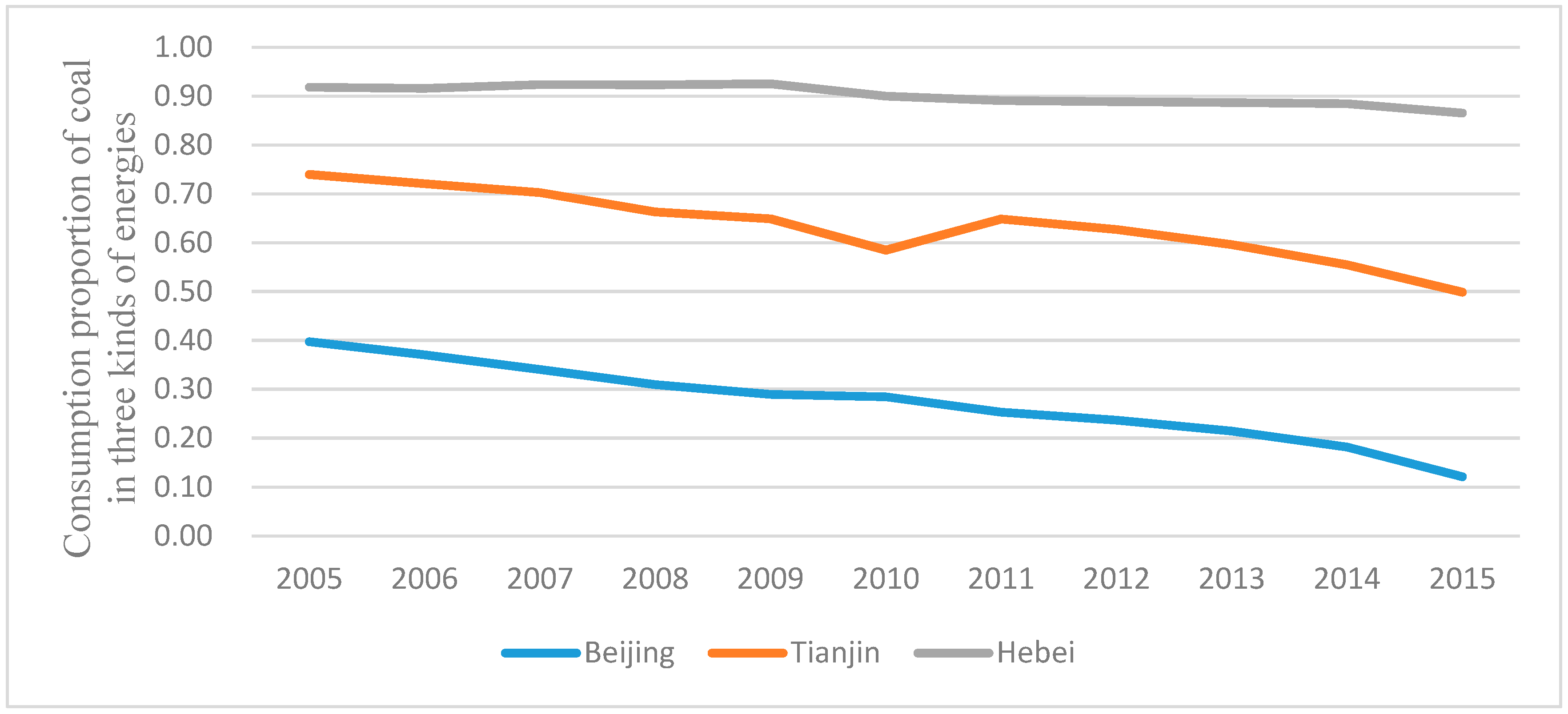
The technical level and energy structure also have important impacts on carbon emissions. Every 1% decrease of unit GDP energy consumption will reduce carbon emissions by about 0.66%. Meanwhile, one percentage point drop of coal’s share in the total energy will cause a drop of about 0.65 percentage points in carbon emissions. The technical level represents the utilization efficiency of energy at the present stage. The improvement of the technical level can reduce unit GDP energy consumption. Among the three kinds of energies, coal has the highest carbon emission coefficient, which means that for generating same amount of energy, the carbon emissions would be far more than the consumption of petroleum or natural gas, when it is generated by coal combustion. Thus, a decrease in the proportion of coal in the total energy would definitely reduce carbon emissions. In China, coal consumption accounts for a large proportion of the total energy production. However, compared to clean energy sources, such as natural gas, coal generates a large number of pollutants during the combustion process, especially when processes of cleaning and desulfurization are not up to standard. Coal increases environment burden, and goes against the realization of the sustainable development of the economy. Besides, energy utilization efficiency is also an important factor for restricting economic development. The World Bank for GDP (constant price purchasing power parity with dollar in 2011/kg petroleum equivalent) provides statistical data regarding unit energy consumption in the main global countries in 2015. For the energy consumption per kilogram petroleum equivalent, the GDP output of Japan was 11.03 dollars; America and India were 7.45 dollars and 8.46 dollars, respectively; however, China was 5.70 dollars. There was a big gap between China and the developed countries, such as America and Japan, etc. China was also lower than India, which is also a developing country. So, energy utilization efficiency is an important path for realizing carbon emission reductions in the future. Regarding energy structure, the main energy of Tianjin and Hebei is still coal. Especially in Hebei Province, coal accounts for more than 90% of the total consumption of the three energy sources. Although it has been declining in recent years, the effects are not yet obvious. In the future, there ought to be greater efforts to change the existing energy consumption pattern in the region, and a greater use of clean energy to replace coal, petroleum, and other high-pollution fossil fuels.

The proportion of the second industry in the regional GDP is down by one percentage point, which will only reduce carbon emissions by 0.0388 percentage points. The optimization of the industrial structure does not have an obvious impact on carbon emissions, which is inconsistent with economic intuition. It is generally recognized that the energy consumption of the second industry is far more than the energy consumption of the third industry. Why does a proportional reduction of the second industry in the regional economy not exert an obvious function in reducing carbon emissions? One possible explanation is that the development level of the third industry in the region at the present stage is still lower than the international level. In other words, it is far from realizing green development. Although the official statistical data of China shows that the proportion of the third industry has exceeded 50% and become the most important strength for driving economic growth, the unreasonable internal structure (too many traditional service industries, a small scale of modern service industries) is still the key factor for restricting its high-end development. In 2015, the added value of services in the Beijing–Tianjin–Hebei region was 3862.474 billion Yuan, of which the traditional service industries, including wholesale and retail trade, transportation and postal services, and accommodation and catering were 6803.61 Yuan, 4072.05 Yuan, and 105.05 billion Yuan respectively. In contrast, the added value of modern service industries such as finance and real estate was 2669.905 billion Yuan. The added value of the traditional service industries accounted for 30.87% of the total output value of the service industry. From the perspective of various regions, the data of Beijing, Tianjin, and Hebei was 20.52%, 35.41%, and 43.52%, respectively. There was a big difference between the regions. In contrast, in 2016, the traditional industry in America only occupied 25.29% of the total output value of the service industry. This shows that the adjustment of economic structure of Hebei and Tianjin should not only focus on the improvement of quantity, it should also pay more attention to the optimization of the service industry structure. The data regarding China comes from the China Statistical Yearbook of 2015, and the data regarding America comes from the United States (US) Bureau of Economic Analysis.

4. Game between Local Governments

The transboundary pollution in the Beijing–Tianjin–Hebei region is serious. Under the administrative governance model of “territoriality”, the transboundary pollution among the regions increases the difficulty of atmospheric environmental pollution control. Generally, the regional government takes high-speed economic growth as its main objective, even at the cost of excessively high environmental pollution. The regional atmospheric environment is a kind of public resource, with the features of non-competition of usage and non-exclusiveness. Each province (city) generates a large amount of atmospheric pollutants, which are emitted by the combustion of fossil fuels that pollutes the environment of the province (city) and the neighboring areas. So, just considering the environment pollution cost in its own region, without considering the negative externality of environment pollution, would certainly underestimate the adverse impact of the pollution. As a result, each region excessively consumes environmental resources, which leads to the occurrence of “the tragedy of the commons”. Due to the serious transboundary atmospheric environment pollution in the region, the effect of any unilateral treatment is not ideal. Therefore, it is an inevitable requirement for the three governments to make joint actions.

According to the empirical analysis results, the critical factors influencing carbon emission are economic development, the technical level, and the energy structure. However, there is big difference between Beijing, Tianjin, and Hebei regarding these aspects (refer to Figure 1, Figure 2 and Figure 3), which lead to the different local governments pursuing different goals. Strict environmental regulations would have an adverse impact on the economic development of the region in the short term. Economic logic dictates that this would increase the cost of production, and the enterprises’ response would be to reduce the number of employees and output, which would hinder the growth of GDP, and increase unemployment. All of this would have a negative impact on the performance of the present government officials. In addition, environmental pollution has a negative externality, which means that unilateral treatment leads to a high cost, and the control effect cannot be ensured. Moreover, environmental treatment has a positive externality, so the phenomenon of “hitchhiking” is inevitable. Therefore, even if common treatment actions are implemented, each government will have no incentive to implement strict governance measures. The dilemma of how to realize coordination and unity between governments in the environment treatment action is the critical factor that will directly influence the effect of atmospheric pollution legislation. Under the administrative governance model of “territoriality”, the local government plays an important role in the implementation of strict environmental protection policies. Whether it supervises and controls the enterprises strictly without any reservation would directly influence the effect of any joint pollution treatment. Through establishing a static game model for the three parties, the paper discovers that a “prisoners’ dilemma” exists in the joint pollution treatment of the three governments. A strict punishment mechanism of the central government on the “malpractice” behavior of the local government would push each party to select the policy with maximum earnings, and benefit the overall improvement of the environmental quality in the region.

The game problem of joint pollution treatment mainly involves three participants (the three governments of Beijing, Tianjin, and Hebei), and each game subject has limited rationality. For strict environmental protection policy, each local government can choose to implement it actively, or negatively. The game subject is a “rational economic man”, who will make the strategic decision in accordance with the principle of its own maximum benefit. We assume that the governments believe that a loose environment supervision policy would bring high-speed economic growth, and that the income of that growth is bigger than the income that would derive from environmental quality improvements under a strict environmental protection policy (this assumption is reasonable, otherwise, why would the atmospheric environmental quality in China be so bad?), i.e., the income of the government under loose environment supervision is 1, and the income of strict supervision is −1. If the neighboring region carries out a strict environmental protection policy, the local government will get 1 unit of income, due to the existence of positive externality. On the contrary, if the neighboring region carries out a loose environmental protection policy, the local government will lose 1 unit of income, due to the existence of negative externality. The central government and local government pursue different interest targets. The local government strives to realize its maximum income, while the target of the central government is to improve the environmental quality of the whole region continuously, so as to realize the sustainable development of the society and the economy. Thus, the more that the regions strictly carry out environmental protection, the more they will conform to the interests of the central government. The central government could supervise the policy implementation of the local government to find out whether the local government carries out a strict environmental protection policy, and could punish the local government for poor implementation. Under a static game (“yes” represents a strict environmental protection policy by the government, while “no” represents a loose environmental protection policy by the government), the regional governments’ income matrix is in

Table 12. The income matrix of regional government under no central government supervision.

	Tianjin	Yes		No
	Hebei	Yes	No	Yes	No
Beijing	Yes	(1, 1, 1)	(−1, −1, 3)	(−1, 3, −1)	(−3, 1, 1)
	No	(3, −1, −1)	(1, −3, 1)	(1, 1, −3)	(−1, −1, −1)

.

The equilibrium solution in Table 12 is (−1, −1, −1), i.e., all three governments choose to implement a loose environmental governance policy, facing the “prisoners’ dilemma”, which will result in the continuous deterioration of environmental quality in the whole region. It does not conform to the requirement of the sustainable development of the economy, and also does not satisfy the demand of the local residents for clean air. If the central government carries out a strict punishment mechanism on the local government that conducts “malpractice” behavior, and makes it lose three unit incomes, then the game matrix is presented in

Table 13. The income matrix of regional government under strict central government supervision.

	Tianjin	Yes		No
	Hebei	Yes	No	Yes	No
Beijing	Yes	(1, 1, 1)	(−1, −1, 0)	(−1, 0, −1)	(−3, −2, −2)
	No	(0, −1, −1)	(−2, −3, −2)	(−2, −2, −3)	(−4, −4, −4)

:

At this time, the Nash equilibrium exists in Table 13, with an equilibrium solution of (1, 1, 1), i.e., the three governments all choose to implement a strict environmental protection policy. The central government realizes the target, which is of benefit for improving the environment quality of the whole region.

5. Conclusions and Policy Suggestion

In this paper, we used multivariate linear regression on a STIRPAT model to explore the impact of economic growth, the technological level, the energy structure, and the industrial structure on the air pollution in the Beijing–Tianjin–Hebei region from 2005 to 2014, and we also established a three-party static game model in order to analyze the related issues of joint pollution control among the regional governments. Some important conclusions were drawn.

First, we found that the rapid economic growth based on magnanimous fossil fuel consumption is the main reason for the deterioration of the atmospheric environment. Although the economic transformation strategy has been proposed in China for many years, the economic development pattern in the region has not changed. If the region still develops its economy in the traditional way, it will inevitably consume a lot of energy, which will burden the environment atmosphere. Therefore, economic restructuring is still the main task of the region, especially for Hebei province.

Second, the optimization of the energy structure and improvement of the technology level can effectively reduce energy carbon emissions, which is conducive to changing the status of the atmospheric pollution in the region. This means that the coal-to-natural gas strategy implemented in the Beijing–Tianjin–Hebei region can play an important role in curbing air pollution. In addition to heating, the government should actively promote new energy in other areas rather than fossil fuels, especially for family cars and city buses. All of this can reduce the consumption demand for highly polluting energy sources such as coal and oil, and contribute to the improvement of the atmospheric environment. In addition, enterprises and governments should take the initiative in introducing advanced production technology, machinery, and equipment in order to improve energy efficiency. Only by actively promoting these two aspects can we effectively alleviate the continuous deterioration of the environmental quality in this region.

Third, more attention should be paid to improving the quality of the tertiary industry, rather than the quantity. Official data shows that the tertiary industry contributes more than 50% of GDP, but our research shows that the tertiary industry in China is still dominated by the traditional tertiary industry, and the development of the high-end service industry is relatively backward. Traditional service industries are highly dependent on energy, which is why although the industrial structure has been continuously optimized, it has not played any significant role in reducing carbon emissions. In the future, the service sector, especially the productive high-end service sector, will have a deeper integration with other industries, such as manufacturing and agriculture. High-end service industries will promote the economy to a low-carbon, high-quality stage.

Forth, cross-border pollution is an important reason for the continued deterioration of the air quality in the Beijing–Tianjin–Hebei region. Joint action between regions can effectively alleviate the continuous deterioration of air pollution, which is based on the premise of the central government earnestly fulfilling its oversight responsibilities. The strict supervision of the central government is an effective mechanism for solve the prisoners’ dilemma in regional cooperation. The central government may set up special inspection agencies in order to conduct regular inspections of enterprises and environmental protection departments in various provinces. This will prompt all of the regional governments to strictly enforce environmental protection policies.