Article

Effects of Bank Lending on Urban Housing Prices for Sustainable Development: A Panel Analysis of Chinese Cities

1
School of Management Engineering, Shandong Jianzhu University, Jinan 250101, China
2
School of Planning, Design and Construction, Michigan State University, East Lansing, MI 48824, USA
3
College of Architecture, Planning and Landscape Architecture, University of Arizona, Tucson, AZ 85721, USA
4
Department of Construction Science, Texas A&M University, College Station, TX 77843, USA
*
Author to whom correspondence should be addressed.
Sustainability 2018, 10(3), 642; https://doi.org/10.3390/su10030642
Submission received: 2 February 2018 / Revised: 20 February 2018 / Accepted: 22 February 2018 / Published: 28 February 2018
(This article belongs to the Section Sustainable Urban and Rural Development)

Abstract

:
Stable home prices are critical to a healthy housing market and sustainable development. Home prices in many Chinese cities have increased dramatically in past decades. The China’s central bank uses two primary monetary controls on overheated housing prices: the bank lending supply and lending rate. However, little to no evidence informs whether the nation-level bank lending controls are effective at the city level. Unlike extant studies that only focus on nation-level effects of such controls, this research analyzes long-run effects on housing prices at the national, regional, and city levels. The authors perform cross-sectional time-series regressions on empirical data from 35 major Chinese cities for the period 2003 to 2015. Results confirm that controlling lending rates is effective as a long-term measure at the national, regional, and city levels, whereas controlling the lending supply is effective as a short-term measure for many cities. Results also reveal that housing prices cause lending supply changes for many regions in a long run and indicate that credit policy often lags in response to housing price changes. Findings show that the effectiveness of bank lending largely varies at the city level, suggesting city-tailed bank lending rather than the centralized controls at the national level.

1. Introduction

Housing is a substantial economic force. In the United States, spending on housing and housing services has tended to represent 15% of GDP. In China, the focus of this paper, housing spending has grown to 8% of GDP. Rapidly increasing home prices are problematic and raise concerns against sustainable development [1], such as increased financial pressure on households and large real-estate bubbles. These high prices have resulted in a disproportional price-to-income ratio that largely exceeds the international guard line [2] and threatens a healthy housing market. An average household looking to buy a house in Shanghai would pay 25 years of income for a 90 m2 apartment. Furthermore, as housing price booms typically lead to busts, a financial crisis may be triggered [3].
Housing is a complex bundled good and changes in pricing indicate the weighted average change in the value of its constituent components [4,5]. Housing has important connections to household behavior, local and national policy, and the environment [6]. A user of all factors of production, housing is routinely associated with consumption of land, energy, and materials. Importantly, as housing has a fixed location, its relative location ties it both to filtering processes [7] and to transportation and the related expenses and externalities [8,9].
Given the complex connectivity between these issues, sustainability in housing has typically been examined as a function of resource and location efficiency. Studies have examined sustainable construction product selection [10]; energy efficiency and the role of eco-certification schemes [11,12]; as well as traditional neighborhood design [13] and walkability [14]. However, as variation in housing supply and home prices, which are metrics describing the bundled consumption of land, housing, and their requisite energy and materials, are associated with inflation [15], there is an opportunity to study sustainability in housing markets as a function of variation in macro-economic conditions such as central government monetary policy. This opportunity is exploited here.
The People’s Bank of China, the central bank, uses monetary controls as primary macroeconomic means to cool overheated housing prices. Limiting the housing loan supply (i.e., bank lending) and increasing the borrow rate are two common monetary policies used to ensure price stability [16]. The central bank can increase the interest rate or reserve requirements to reduce the liquidity of commercial banks. In response, the banks cut back on the supply of mortgages and loans and effectively limit lending [17]. The central bank adjusted the borrowing rate for housing loans 24 times from 2003 to 2015 and gradually raised the down payment baseline for a second home from 30% to 60% in the same period. However, housing prices in China continued to increase for decades.
Exploring the inflation-housing supply-housing consumption-sustainability relationship, the objective of this research is to identify the causal effects of bank lending on urban housing prices at city level across varying periods. Unlike extant research mainly focuses on nation-level effects, this study examines such effects of bank lending at national, regional, and city levels. We hypothesize that the causality between bank lending and housing prices varies at city level. We believe that a centralized bank lending policy at the national level is less effective for a sustainable urban housing market. In the context of recent examinations of the influence of various economic policies on housing prices, this paper uses the Chinese property market as the lens through which we examine the effectiveness of central bank monetary policy. More specifically, we investigate whether and how the lending supply through housing loans and the lending rate through interest rates affect housing prices in 35 major Chinese cities. Our argument is that in influencing home prices, the central bank can help to create a more sustainable future for China by shaping the housing supply—and as a result, the utilization of land, materials, and energy.

2. Literature Review

Housing markets and prices are complex and connected to a myriad of factors and forces. Consequently, the literature review below summarizes literature germane to housing price variation in Chinese markets and the role of monetary policy in shaping home prices in a global context. It also describes how sustainability in housing has typically been studied and the opportunity that this paper seizes related to macro-economic forces and their ability to shape a sustainable future in housing. Otrok and Terrones (2005) studied the dynamic properties of house prices, interest rates and macroeconomic for 13 industrial countries. The results showed housing price comovement in 13 industrial countries was related with interest rates, but the response of housing price on U.S. monetary shocks is different between the U.S. and the rest of the world [18]. Beltratti and Morana (2010) investigated the linkage between housing prices and macroeconomic developments for the G-7. The results showed the linkage between house prices and macroeconomic developments is bidirectional, with investment showing in general a stronger reaction than consumption and output to real house price shocks [19]. Tsatsaronis and Zhu (2004) studied the impact of macroeconomic factors on housing prices dynamics for several industrialized countries. The results showed house prices were more sensitive to short-term rates, and more aggressive lending practices are associated with stronger feedback from prices to bank credit [15]. Manganelli et al. (2014) used VAR model to investigate the relationships between selling and rental prices of the Italian housing market. The results showed housing prices were highly responsive to short-term real interest rates [20]. Manganelli and Tajani (2015) used VAR model to analysis the impact of economic system on housing prices trend in the USA and in Italy. The results showed the lending rate can contribute to explaining the variability of the Italian housing prices, but has no effect in the American model [21].
The Chinese property markets and government interventions used to guide and manage them have been the subject of a growing body of scholarship [22,23,24]. From gentrification patterns [25], to the role of city mayors in moderating environmental externalities [26], to the creation of repeat sales indices using emerging data [27], researchers have investigated and explored the complexities of one of the fastest growing residential markets on the planet. One vein of the extant literature has sought to explain factors associated with variation in Chinese home prices. Zheng at el. [26] analyzed home price changes using foreign direct investment, ambient air pollution, and wage metrics—finding evidence of a shift from producer cities to consumer cities. Li and Mao [22] provided a summary of housing policy interventions and observed patterns of mobility within residential markets. Shen [28] examined the significant price to income ratio growth relative to other developed nations and observed that affordability in Chinese markets remained strong. Further, Ren et al. [29] applied an auto-regression test for the presence of a housing market bubble and found no evidence that prices exceeded intrinsic values. Wu et al. [25] analyzed supply and demand factors associated with price movements and noted the importance of land in rising housing prices. Zhou et al. [30] observed evidence of anchoring behavior in the Chengdu housing market as non-local investors tended to over-pay for similar quality housing units.
Relatedly, both in and out of the Chinese context, scholars have specifically investigated whether monetary controls effectively affect overhead housing prices in the long term, with varying results. Some have asserted that the bank lending supply causes housing price changes [3,31,32,33,34]. In other words, housing prices are sensitive to mortgage rates, credit capacity, loan supply, and loan-to-value ratios. Contrasting studies [35,36,37] highlight that housing prices lead to changes in the lending supply through the wealth effect. Moreover, some point out a mutual dependence between housing prices and the lending supply [38], whereas others underline the lending rate as the cause of housing price increases rather than the lending supply [39,40]. The effect of the lending rate on housing prices varies depending on investment need, metropolitan area [41], city administration, and geographic region [26,41]. Specifically focused on the role of central bank economic policy in moderating Chinese housing prices, Li and Xu [42] found restrictive loans and prices to be effective pricing controls while restricted purchases were not. Chiang [43] identified a strong association between the role of expansionist monetary policy and rising residential rents. It is from this foundation, that our paper seeks to extend and contribute to the conversation on the influence of central bank policy on housing prices by focusing on monetary policy—namely, lending supply and interest rates at the city level.
Given that housing is a substantial consumer of all factors of production—specifically land, building materials, labor, and energy (both with respect to production and operation)—scholars have tended to study sustainability in housing with resource efficiency questions. Broadly, the resource efficiency questions have focused on the demand for and the value proposition of sustainable housing. For example, analyses examined the diffusion patterns (and as a result the demand for) sustainable construction technologies [10] and housing in the U.S. [11]—observing that demand was influenced by climate, policy, and economic conditions. Relatedly, studies have suggested that homes with sustainable features and locations created competitive advantage for owners [13,44,45,46,47,48]. This competitive advantage has carried over to lenders as borrowers on energy efficient homes and homes in more walkable areas tended to be less likely to default on their mortgages than borrowers on similar traditional homes [12,14]. Naturally, these connect with research that noted geography and location [6,8,9], taxation schemes [49], and local policy [50] are all associated with variation in home prices. Moreover, there are signals from outside of housing suggesting that urban spatial structure and urban form shape transportation patterns, greenhouse gas emissions, and public health [51,52].
In the context of the observed relationships between housing supply, housing prices, policy, and sustainability, this paper utilizes a non-traditional pathway. Instead of focusing on the micro-economic choices of individuals and firms and how each of those reflect elements of resource efficiency, this paper focuses on the role of macro-economic effects—namely, central government monetary and lending policies and their ability to influence housing supply and prices. The premise of the argument is a resource efficiency one; that is, to the extent monetary policy controls can shape housing prices and supply (demand for housing), central governments can reduce the production of housing and the land, energy, and materials included therein.

3. Materials and Methods
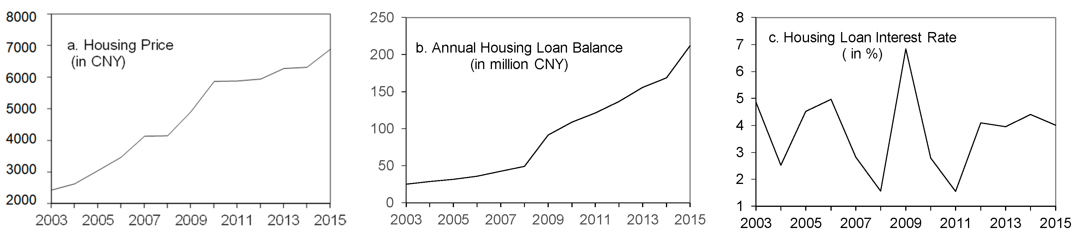
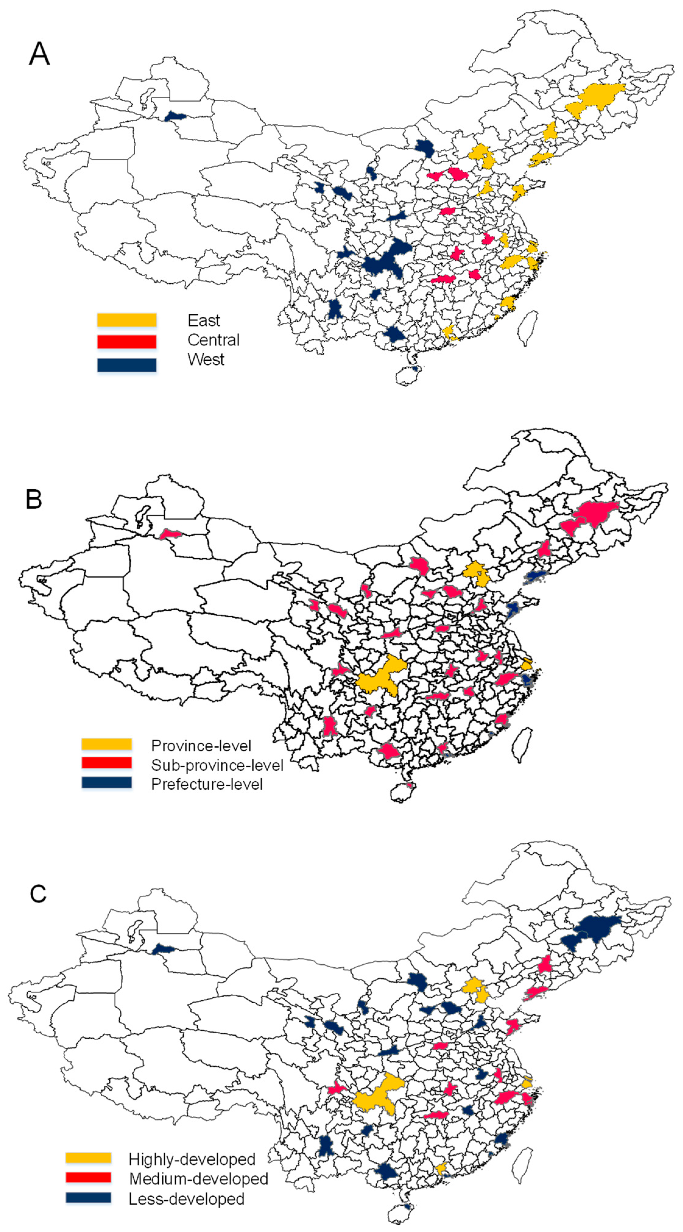
3.1. Data

Data used in this study include annual city-level house prices, lending supply, lending rates, and GDP. Data were collected from 35 major cities in China across 13 years (2003–2015). Specifically, house prices and GDP data were retrieved from the China Statistical Yearbook 2003–2016; bank lending balance data were from the China City Statistical Yearbook 2003–2016; and lending rates were calculated using the daily rate retrieved from the central bank of China. The simple average method was used to calculate housing prices which were the ratio between housing sales and housing sales volume. All monetary data were adjusted to the base year 2003 using the consumer price index (CPI). There were no missing data.
Figure 1 exhibits descriptive statistics about the nation-level trends in average housing prices, lending supply, and loan rates from 2003 to 2015. The results show that the home prices in Chinese cities have increased dramatically since 2003 [1]. According to China’s National Bureau of Statistics, urban housing prices in China increased more than 9% annually from 2003 to 2015. In contrast, prices in the United States increased 5% in the same period [2,53]. Similarly, the annual lending loan balances increased sharply along the growth of housing prices. In contrast, the lending rate fluctuated between 1% and 7% during the same period.
The 35 cities are Beijing (BJ), Changchun (CC), Chengdu (CD), Chongqing (CQ), Changsha (CS), Dalian (DL), Fuzhou (FZ), Guiyang (GY), Guangzhou (GZ), Haikou (HA), Hefei (HF), Hohhot (HO), Harbin (HR), Hangzhou (HZ), Jinan (JN), Kunming (KM), Lanzhou (LZ), Ningbo (NB), Nanchang (NC), Nanjing (NJ), Nanning (NN), Qingdao (QD), Shanghai (SH), Shijiazhuang (SJ), Shenyang (SY), Shenzhen (SZ), Tianjin (TJ), Taiyuan (TY), Wuhan (WH), Urumqi (UR), Xi’an (XA), Xiamen (XM), Xining (XN), Yinchuan (YC), and Zhengzhou (ZZ). We chose these 35 cities as samples because this sample of cities is geographically diversified, represents nearly 50% of GDP growth, and contains substantial home price variation—permitting analysis of various typologies to be conducted [26].
We classify the 35 cities by geographic location, administrative hierarchy, and economic development to analyze regional variances of the effects of the monetary controls. Figure 2 maps city distributions using the three classifications. Figure 2A groups cities by geography (i.e., eastern, central, and western regions), showing that urban development in China varies based on distance to the eastern coast. In other words, the eastern region typically has more advanced industries, infrastructure, and control systems than other areas, and it includes 16 cities. Figure 2B groups cities by administrative hierarchy (from high to low): province-level municipalities, sub-province-level cities, and prefecture-level cities. In China, political administration plays an important role in macroeconomic controls. That is, higher-level cities often have more resources (e.g., financial reserves) to implement controls. Specially, our samples include all four province-level municipalities, 26 sub-province-level cities, and 5 prefecture-level cities. Figure 2C groups cities by development level: highly-developed cities, medium-level cities, and less-developed cities.

3.2. Analytical Methods

We used a panel data analysis (also known as a cross-sectional time-series data analysis). Three independent variables (i.e., lending supply, the lending rate, and annual GDP) were used to identify the long-term effects of monetary controls on housing prices at the national, regional, and city levels over time. Considering previous research [17,32], our hierarchical regression model is represented as:
ln H i t = α i + β 1 i ln L i t + β 2 i R i t + β 3 i ln G D P i t + ε i t
where Hit represents real housing prices in city i in year t; GDPit represents real GDP (in CNY); Lit represents the bank lending balance using GDP in city i in year t; Rit represents the real lending rate in city i in year t; β1i, β2i, and β3i are estimated coefficients; and εit is random disturbance. GDP is used as a control variable in the regression. We divided the lending balance using GDP to avoid possible multicollinearity [17]. We used STATA software v14 (StataCorp LLC, College Station, TX, USA) for the statistical analysis.
We followed a three-step procedure to perform the panel data analysis: (1) a panel unit root test; (2) a panel cointegration test; and (3) a panel Granger causality test. The unit root test examines variable stationarity and thus enables us to confirm the estimation validity and avoid spurious regression. The LLC test [54], ADF-Fisher test [55], and PP-Fisher test [56] were used for the unit root test. The cointegration test is used to judge the existence of a long-term equilibrium relationship among variables. The Pedroni technique [57] was used in this study to examine the cointegration of bank lending at national and regional levels. Statistics for the Pedroni test include Panel-v, Panel-rho, Panel-PP, Panel-ADF, Group-rho, Group-PP, and Group-ADF, of which Panel-ADF and Group-ADF are more reliable and preferred [58]. The panel Granger test is used to identify causal relationships among variables when variables pass the cointegration test. The results from unit root test and cointegration test are used to ensure the validity of Granger causality. In this study, we used a panel vector error correction model (VECM) to test Granger causality [59] among housing prices, the lending supply, and the lending rate. VECM allows to identify both long-run causality by testing the error correction term ECT (−1) and short-run causality by testing the F-statistic. The VECM is written as follows:
Δ y i t = θ i j + λ i t E C T i t 1 + k ξ i t Δ y i t 1 + k φ i t Δ x i t 1 + μ i t
where ∆ represents the first difference; θij is the constant term; λit, ξit, and ϕit are estimated parameters; ECTit−1 is the lagged error correction term; and µit is white noise.
Three analytical techniques were used to estimate the parameters: the constant coefficient model (Equation (3)), varying intercept model (Equation (4)), and varying coefficient model (Equation (5)). The three models use different intercepts and slopes [60]. The constant coefficient model estimates constant intercepts and slopes; the varying intercept model has different intercepts but the same slopes; and the varying coefficient model contains separate intercepts and slopes. The varying coefficient model is a widely adopted tool for analyzing the relation between a response and a group of covariates [61]. The model contains similar structure and interpretability to a traditional linear regression model but is more flexible owing to the infinite dimensionality of its corresponding parameter spaces [62,63].
ln H i t = α + β 1 ln L i t + β 2 R i t + β 3 ln G D P i t + ε i t
ln H i t = α i + β 1 ln L i t + β 2 R i t + β 3 ln G D P i t + ε i t
ln H i t = α i + β 1 t ln L i t + β 2 t R i t + β 3 t ln G D P i t + ε i t
where i denotes city (i = 1, 2, …, 35); t denotes year (t = 2003, 2004, …, 2015); and k denotes variable (k = 1, 2, and 3) in Equation (1). The following analytical hypotheses were used to determine model selection by testing the F1 and F2 statistics:
H 1 : β k 1 = β k 2 = = β k N
H 2 : α 01 = α 02 = = α 0 N , β k 1 = β k 2 = = β k N
F 1 = ( S 2 S 1 ) / [ ( N 1 ) K ] S 1 / ( N T N ( K + 1 ) ) ~ F [ ( N 1 ) k , N ( T K 1 ) ]
F 2 = ( S 3 S 1 ) / [ ( N 1 ) ( K + 1 ) ] S 1 / ( N T N ( K + 1 ) ) ~ F [ ( N 1 ) ( K + 1 ) , N ( T K 1 ) ]
where S1, S2, and S3 represent the residual sum of squares in Equations (3)–(5), respectively; N represents the number of cross sections; T represents time; and K represents the number of independent variables. If F1 is smaller than the related critical value under a given confidence level, H2 is accepted and the constant coefficient model (Equation (3)) is selected; otherwise, it is necessary to test H1. If F2 is smaller than the related critical value under a given confidence level, H1 is accepted and the varying intercept model (Equation (4)) is selected; otherwise, the varying coefficient model (Equation (5)) is selected [64]. The F1/F2 settings ensure the validity and reliability of analytical results from models.

4. Results

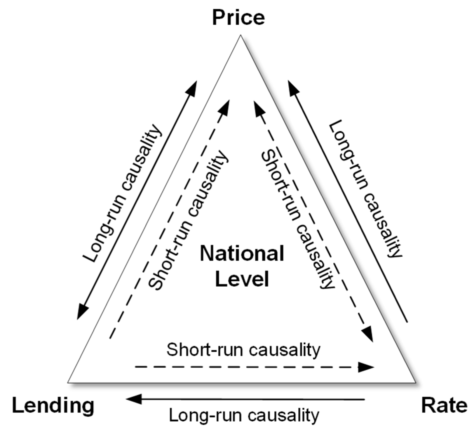
4.1. Nation-Level Effects

Table 1 lists the results from the panel unit-root test. The results indicate that the four variables are panel non-stationary in the level values but panel-stationary in the first difference at a 5% significance. Therefore, we integrated the four variables into order 1, namely, I(1), and conducted panel cointegration tests in the following step.
Table 2 exhibits the results of the Pedroni cointegration test on the national panel. The results indicate that the null was rejected (i.e., no cointegration among variables) because at least four statistics (including Panel ADF and Group ADF) reject the null hypothesis at the 1% significance. The finding suggests a long-run equilibrium relationship between any pair of housing prices, lending supply, and lending rates. In other words, causality exists and panel Granger causality tests can be conducted.
Figure 3 illustrates the results of Granger causality tests on the national panel using VECM. The results show a long-run bi-directional causal relationship between housing prices and the lending supply (termed Lending hereafter) and a short-run bi-directional causal relationship between housing prices and the interest rate (termed Rate hereafter). The results indicate one-way short-run causal relations from Lending toward both housing prices and Rate. Similarly, the results indicate one-way long-run causal relations from Rate toward both housing prices and Lending. The finding confirms the effects of the two monetary-control approaches on housing prices at the national level in China. Our finding also reveals the variation in efficiency of the two monetary controls: the lending supply is effective in the short run, and the interest rate is effective in the long run. Furthermore, lending constraints result in corresponding changes in interest rates in the short term, whereas interest rates cause lending constraints in the long run. The finding suggests policy implications for nation-level decision makers, as monetary controls on housing loan amounts (e.g., reserve requirements, asset discount rates, and down payments) can provide immediate effects on housing prices. In contrast, a long-term healthy housing market relies on effective controls using lending rates at the national level.

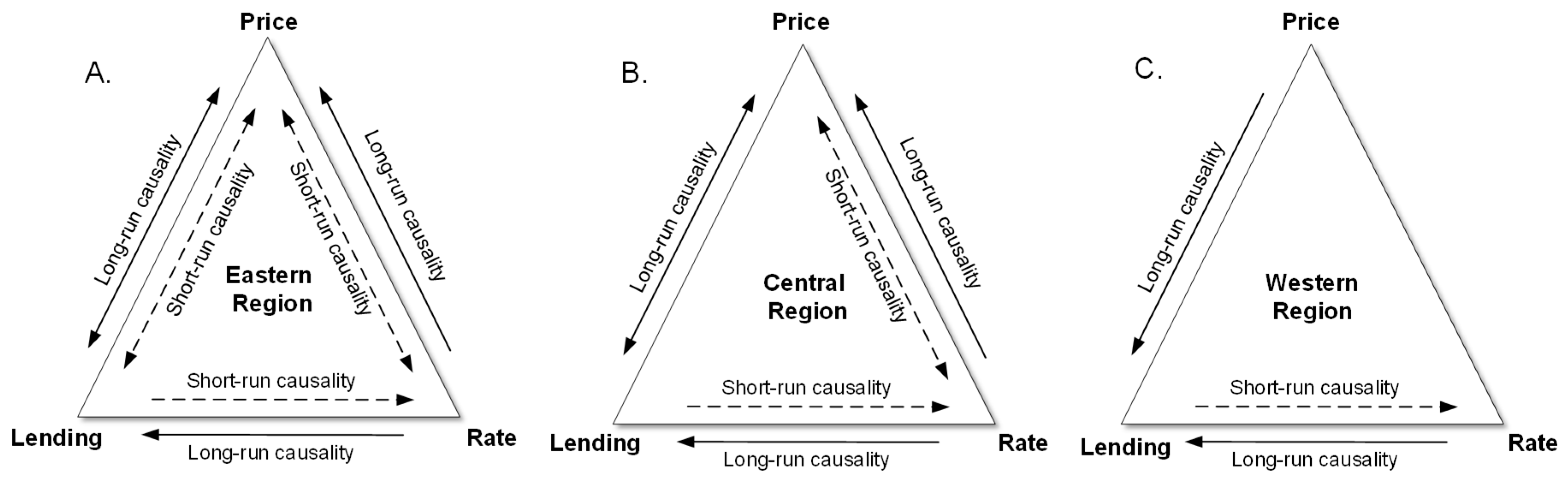
4.2. Region-Level Effects by Geographical Location

Table 3 exhibits the results of a Pedroni cointegration test on geographic regions. The results accept cointegration among variables in the eastern, central, and western regions because at least four Pedroni statistics (including Panel ADF and Group ADF) reject the null at 5% significance. The finding suggests a long-run equilibrium relationship between any pair of housing prices, lending supply, and the interest rate in all geographical regions. In addition, the panel unit root test is satisfied as in Section 4.1. Therefore, region-level panel Granger causality tests can be performed.
Figure 4 illustrates the results of Granger causality tests on geographic regions. Like findings from the national panel, results from all regional panels show that the lending supply affects the interest rate in the short run but is affected by the interest rate in the long run. Different from the findings of the national panel, results from the eastern and central regions identify only one one-way causality from the interest rate to housing princes in the long run. The finding confirms the efficiency of interest rate as an effective long-term control in eastern and central China. However, the housing loan supply does not work effectively as a monetary control in these regions. Results from the western region indicate that both lending supply and the interest rate are not effective measures for controlling housing prices. Conversely, the lending amount is impacted by rising housing prices in this region, suggesting a lagging effect from the control. Given that the western region has experienced high-speed economic growth and urbanization in the past decade, the finding suggests that no monetary controls function when a region is under rapid development owing to higher expectations for real-estate investment.

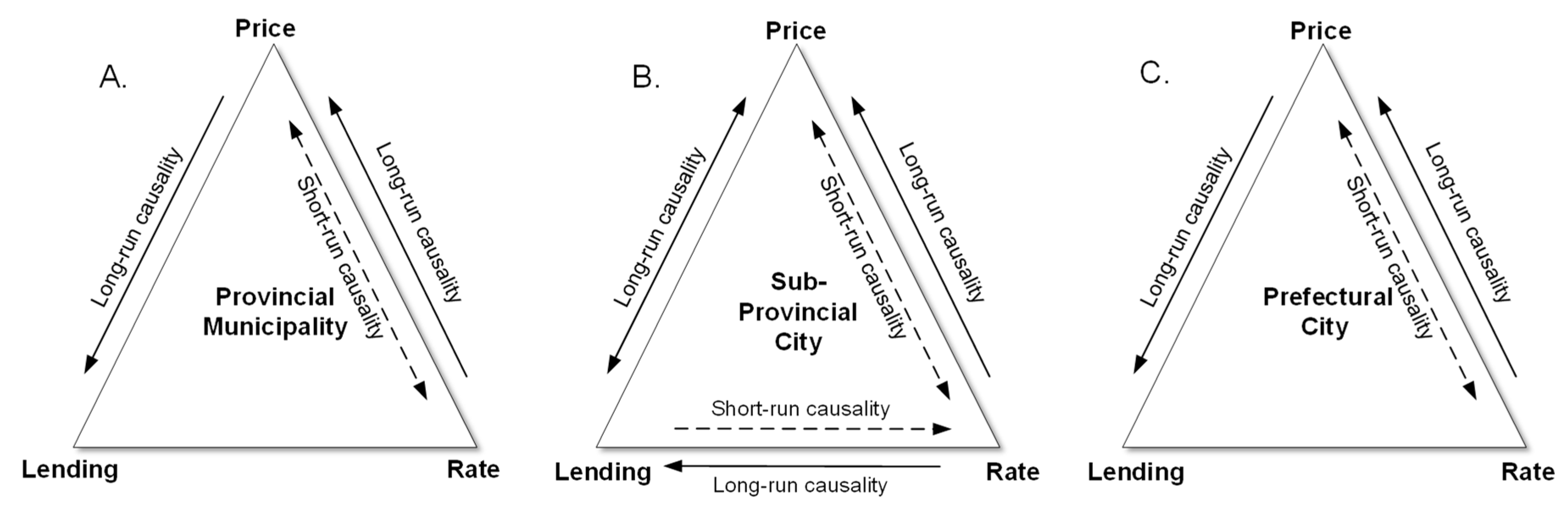
4.3. Region-Level Effects by Administrative Hierarchy

Table 4 exhibits the results of a Pedroni cointegration test on administrative hierarchy. The results accept cointegration among variables in provincial, sub-provincial, and prefectural cities because at least four Pedroni statistics (including Panel ADF and Group ADF) reject the null at 5% significance. The finding suggests a long-run equilibrium relationship between any pair of housing prices, lending supply, and the interest rate in cities of all administrative hierarchies. Because the panel unit root test was satisfied, region-level panel Granger causality tests can be performed.
Figure 5 illustrates the results of Granger causality tests on administrative hierarchy. Similar to the findings from the national panel, results from all administrative levels delineate a long-run causality from the interest rate to housing prices and short-run interactions between them. This finding confirms that the interest rate is an effective control measure in the long run for all levels of administration. Different from the findings of the national panel, results from all administrative levels do not show an effect from the lending supply to housing prices but that changes in housing prices determine the corresponding level of housing loan supply for provincial municipalities and prefectural cities in the long run. This finding suggests that banks’ credit policies are not effective for either province-level cities owing to bureaucracy or prefecture-level cities owing to weaker administration or less resources.

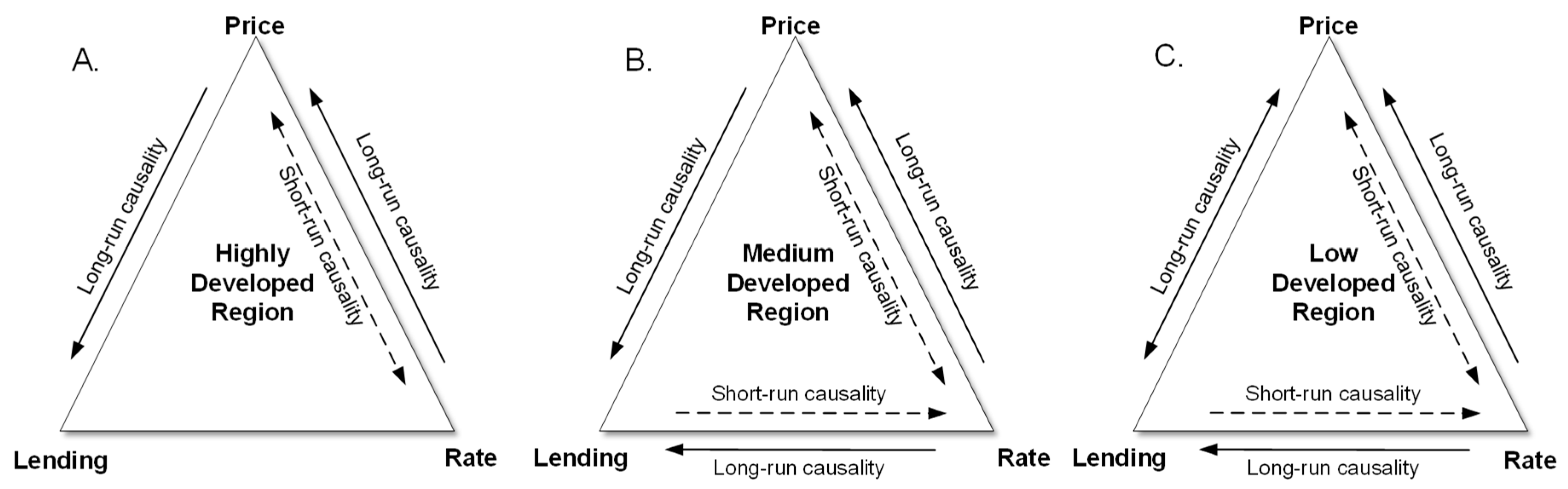
4.4. Region-Level Effects by Level of Economic Development

Table 5 displays the results of a Pedroni cointegration test on regions grouped by level of economic development. The results accept cointegration among variables in high-, medium-, and low-level cities because at least four Pedroni statistics (including Panel ADF and Group ADF) reject the null at the 5% significance. The finding suggests a long-run equilibrium relationship between any pair of housing prices, lending supply, and the interest rate in cities across all development levels. Because the panel unit root test was satisfied, region-level panel Granger causality tests can be performed.
Figure 6 illustrates the results of pairwise Granger causality tests on regions across development levels. Similar to the findings from the national panel, results from all economic levels delineate a long-run causality from the interest rate to housing prices and short-run interactions between them. This finding confirms that the interest rate is an effective measure for long-run controls across all levels of economic development. Differing from national panel findings, the results in this section do not indicate that the lending supply is an effective control on housing prices. Moreover, in the long term, housing loan supply in highly and medium-developed regions follow the change of housing prices. This finding suggests that lending policy (e.g., loan constraints) in developed cities often lag behind when responding to housing price increases. In other words, homebuyers expect a higher return from real-estate investment when the economy is positive, implying that policymakers should control the housing loan supply more proactively and systematically in response to such situations.

4.5. City-Level Effects

The results indicate that the varying coefficient model (Equation (5)) is selected for coefficient estimation, and S1 = 2.9018, S2 = 6.540, and S3 = 101.914. According to Equations (6) and (7), F1 (F1 = 3.871) is greater than the critical value at a 5% confidence level (i.e., F0.05 (136, 315) = 1.262), and F2 is greater than the critical value at a 5% confidence (i.e., F0.05 (102, 315) = 1.291). Thus, we selected the varying coefficient model to estimate coefficients (i.e., β1 for the lending supply and β2 for the interest rate) listed in the regression model (Equation (1)).
Table 6 presents the coefficient estimation for all 35 cities. We categorized the 35 cities into four groups based on the significance of coefficients. Group I includes seven cities for which β1 and β2 are both statistically significant, indicating that controls on both lending supply and the interest rate are effective. Group II includes seven cities for which only β1 is statistically significant, indicating that only the lending supply control is effective. Group III includes one city for which only β2 is statistically significant, indicating that only the interest rate control is effective. Group IV includes 20 cities for which β1 and β2 are both not statistically significant, indicating that no controls perform effectively.
The results in Table 6 show that the significant coefficients for the lending supply (β1) in most cities (except KM) are positive, indicating correlation in the same direction. That is, housing prices rise when the lending supply increases. The finding suggests that limiting the amount of housing loans available in the market is an effective monetary control for the 14 cities in Groups I and II. The effectiveness of controlling the lending supply is low because β1 < 1.0 for these cities (i.e., CQ, FZ, HA, HR, HZ, KM NB, SH, SJ, SZ, SY, UR, XM, and YC). The results also show that the significant coefficients for the interest rate (β2) in all cities are negative, indicating inverse correlation. That is, housing prices decrease when the interest rate increases. The finding suggests that lowering lending rates for housing loans is an effective monetary control for the eight cities in Groups I and III. Specifically, controlling lending rates is effective because β1 < −1 for the affective cities (HA, HZ, NB, SY, SZ, UR, WH, and XM). Combining the findings indicates that although controlling the lending supply is less effective than controlling interest rates, controlling the lending supply works in a greater number of cities (i.e., 14 vs. 8). Monetary controls are not effective for 20 out of 35 cities in this study, suggesting that the city-level controls are less likely to beat the “hot money” controlled by investors who actively seek short-term returns from the growing real-estate market in China.

5. Conclusions

We conducted a cross-sectional time-series study to identify the effects of two primary monetary controls—lending supply and the lending rate—on housing prices in urban China. Unlike studies that isolate their analysis to nation-level effects, we analyzed the long-run and short-run causality of lending at national, regional, and city levels. Our data were from 35 major cities in China over the period 2003–2015. Particularly, we examined region-level effects by geographic location, administrative hierarchy, and level of economic development. The major contribution of this study is that we have identified the variance of lending policy on housing prices at the city-level. That is, sustainable urban development relies a more innovative and city-tailed bank lending policy [65]. In other words, city and local banks should have more authorities to develop effective lending policies.
Our results confirm that to cool overheated housing prices in China, controlling lending rates is more effective than controlling the lending supply as a long-term measure. Specifically, at the national level, controls on both the lending supply and the lending rate are effective on housing prices, but they work differently. That is, controlling the lending supply is more effective in the short run, whereas controlling the lending rate is more effective in the long run. At the regional level, controlling the lending rate is effective in eastern and central China, whereas controlling the lending supply is not effective in all geographic regions. Furthermore, controlling the lending rate is effective in all administrative regions, whereas controlling the lending supply does not work well; in addition, controlling the lending rate is effective in highly, medium-, and less-developed economic regions, whereas controlling the lending supply is not. However, adjusting either the lending supply or the lending rate are not an effective approach to short-term controls at the regional level. At the city level, we found that controlling the lending rate is more effective than controlling the lending supply but affects fewer cities.
We found that in many regions, housing prices cause changes in housing loan supply in the long run. This finding suggests that credit policies (e.g., loan constraints) often lag in response to housing price increases. Homebuyers expect higher returns from real-estate investments, implying that policymakers should control the housing loan supply more proactively and systematically in response to such situations. In China, especially in big cities, housing has become an investment rather than solely a consumption good; thus, households are willing to borrow more when they expect housing prices to remain constant or increase [66]. Housing is also valuable collateral, so banks are willing to lend more during housing price increases [67]. Moreover, given State ownership of land, it is critical to view the results here in their legal and property rights context—which differs from foils such as that of the United States [65].
We found considerable variances in the effectiveness of controls across cities. In particular, monetary controls are not effective for 20 out of 35 cities in China. This finding shows the weakness of city-level controls when fighting “hot money” controlled by cross-regional investors seeking short-term returns from the housing market in China. In other words, a centralized macroeconomic regulation at national level seems less sustainable and effective to cities. Therefore, this finding provides practical implications for policymakers in China and similar developing countries [68] for sustainable urban development while retaining a healthy housing market.
Many future studies can extend this research. First, intelligent simulation tools that can be used to predict housing price changes given certain monetary controls should be developed. These tools will be informative and productive for decision makers when planning monetary control strategies. Second, the effects of monetary controls on a segmented housing market should be investigated. For example, some controls may be especially effective on certain type of properties.

Acknowledgments

The authors are grateful to the supports from the National Natural Science Foundation of China (#71403150) and the Shandong Humanities and Social Science Research Program (#J13WG02).

Author Contributions

Yongsheng Jiang and Dong Zhao conceived, designed, analyzed, and wrote the paper. Andrew Sanderford supported housing policies and implications in literature review and discussions. Jing Du supported data analysis. All authors have read and approved the final manuscript.

Conflicts of Interest

The authors declare no conflict of interest.

References

  1. Gan, X.; Zuo, J.; Wu, P.; Wang, J.; Chang, R.; Wen, T. How affordable housing becomes more sustainable? A stakeholder study. J. Clean. Prod. 2017, 162, 427–437. [Google Scholar] [CrossRef]
  2. Glaeser, E.; Huang, W.; Ma, Y.; Shleifer, A. A real estate boom with Chinese characteristics. J. Econ. Perspect. 2017, 31, 93–116. [Google Scholar] [CrossRef]
  3. Cerutti, E.; Dagher, J.; Dell’Ariccia, G. Housing finance and real-estate booms: A cross-country perspective. J. Hous. Econ. 2017, 38, 1–13. [Google Scholar] [CrossRef]
  4. Rosen, S. Hedonic prices and implicit markets: Product differentiation in pure competition. J. Political Econ. 1974, 82, 34–55. [Google Scholar] [CrossRef]
  5. Bostic, R.W.; Longhofer, S.D.; Redfearn, C.L. Land leverage: Decomposing home price dynamics. Real Estate Econ. 2007, 35, 183–208. [Google Scholar] [CrossRef]
  6. Saiz, A. The geographic determinants of housing supply. Q. J. Econ. 2010, 125, 1253–1296. [Google Scholar] [CrossRef]
  7. Somerville, C.T.; Holmes, C. Dynamics of the affordable housing stock: Microdata analysis of filtering. J. Hous. Res. 2001, 12, 115–140. [Google Scholar]
  8. Mills, E.S. An aggregative model of resource allocation in a metropolitan area. Am. Econ. Rev. 1967, 57, 197–210. [Google Scholar]
  9. Muth, R.F. Cities and Housing: The Spatial Pattern of Urban Residential Land Use; University of Chicago Press: Chicago, IL, USA, 1969. [Google Scholar]
  10. Koebel, C.T.; McCoy, A.P.; Sanderford, A.R.; Franck, C.T.; Keefe, M.J. Diffusion of green building technologies in new housing construction. Energy Build. 2015, 97, 175–185. [Google Scholar] [CrossRef]
  11. Sanderford, A.R.; McCoy, A.P.; Keefe, M.J. Adoption of Energy Star certifications: Theory and evidence compared. Build. Res. Inf. 2018, 46, 207–219. [Google Scholar] [CrossRef]
  12. Kaza, N.; Quercia, R.; Tian, C. Home Energy Efficiency and Mortgage Risks. J. Policy Dev. Res. 2014, 16, 279–299. [Google Scholar]
  13. Tu, C.C.; Eppli, M.J. An empirical examination of traditional neighborhood development. Real Estate Econ. 2001, 29, 485–501. [Google Scholar] [CrossRef]
  14. Rauterkus, S.Y.; Thrall, G.I.; Hangen, E. Location efficiency and mortgage default. J. Sustain. Real Estate 2010, 2, 117–141. [Google Scholar]
  15. Tsatsaronis, K.; Zhu, H. What drives housing price dynamics: Cross-country evidence. BIS Q. Rev. 2004, 65–78. [Google Scholar]
  16. Kashyap, A.K.; Stein, J.C. Monetary policy and bank lending. In Monetary Policy; The University of Chicago Press: Chicago, IL, USA, 1994; pp. 221–261. [Google Scholar]
  17. Oikarinen, E. Household borrowing and metropolitan housing price dynamics-Empirical evidence from Helsinki. J. Hous. Econ. 2009, 18, 126–139. [Google Scholar] [CrossRef]
  18. Otrok, C.; Terrones, M.E. House Prices, Interest Rates and Macroeconomic Fluctuations: International Evidence. 2005. Available online: https://www.frbatlanta.org/-/media/documents/news/conferences/2005/housing2005/otrokterrones.pdf (accessed on 24 January 2018).
  19. Beltratti, A.; Morana, C. International House Prices and Macroeconomic Fluctuations. J. Bank. Financ. 2010, 34, 533–545. [Google Scholar] [CrossRef]
  20. Manganelli, B.; Morano, P.; Tajani, F. House Prices and Rents. The Italian experience. WSEAS Trans. Bus. Econ. 2014, 11, 219–226. [Google Scholar]
  21. Manganelli, B.; Tajani, F. Macroeconomic variables and real estate in Italy and USA. Ital. J. Reg. Sci. 2015, 14, 31–48. [Google Scholar] [CrossRef]
  22. Li, S.; Mao, S. Exploring residential mobility in Chinese cities: An empirical analysis of Guangzhou. Urban Stud. 2017, 54, 3718–3737. [Google Scholar] [CrossRef]
  23. Zou, G.L.; Chau, K.W. Determinants and sustainability of house prices: The case of Shanghai, China. Sustainability 2015, 7, 4524–4548. [Google Scholar] [CrossRef] [Green Version]
  24. Chen, A. China’s urban housing reform: Price-rent ratio and market equilibrium. Urban Stud. 1996, 33, 1077–1092. [Google Scholar] [CrossRef]
  25. Wu, J.; Gyourko, J.; Deng, Y. Evaluating the risk of Chinese housing markets: What we know and what we need to know. China Econ. Rev. 2016, 39, 91–114. [Google Scholar] [CrossRef]
  26. Zheng, S.; Kahn, M.E.; Liu, H. Towards a system of open cities in China: Home prices, FDI flows and air quality in 35 major cities. Reg. Sci. Urban Econ. 2010, 40, 1–10. [Google Scholar] [CrossRef]
  27. Guo, X.; Zheng, S.; Geltner, D.; Liu, H. A new approach for constructing home price indices: The pseudo repeat sales model and its application in China. J. Hous. Econ. 2014, 25, 20–38. [Google Scholar] [CrossRef]
  28. Shen, L. Are house prices too high in China? China Econ. Rev. 2012, 23, 1206–1210. [Google Scholar] [CrossRef]
  29. Ren, Y.; Xiong, C.; Yuan, Y. House price bubbles in China. China Econ. Rev. 2012, 23, 786–800. [Google Scholar] [CrossRef]
  30. Zhou, X.; Gibler, K.; Zahirovic-Herbert, V. Asymmetric buyer information influence on price in a homogeneous housing market. Urban Stud. 2015, 52, 891–905. [Google Scholar] [CrossRef]
  31. Reichert, A.K. The impact of interest rates, income, and employment upon regional housing prices. J. Real Estate Financ. Econ. 1990, 3, 373–391. [Google Scholar] [CrossRef]
  32. Liang, Q.; Cao, H. Property prices and bank lending in China. J. Asian Econ. 2007, 18, 63–75. [Google Scholar] [CrossRef]
  33. Chu, Y. Credit constraints, inelastic supply, and the housing boom. Rev. Econ. Dyn. 2014, 17, 52–69. [Google Scholar] [CrossRef]
  34. Favara, G.; Imbs, J. Credit supply and the price of housing. Am. Econ. Rev. 2015, 105, 958–992. [Google Scholar] [CrossRef]
  35. Bernanke, B.S.; Gertler, M. Agency costs, collateral, and business fluctuations. Am. Econ. Rev. 1986, 79, 14–31. [Google Scholar]
  36. Kiyotaki, N.; Moore, J. Credit cycles. J. Polit. Econ. 1997, 105, 211–248. [Google Scholar] [CrossRef]
  37. Gerlach, S.; Peng, W. Bank lending and property prices in Hong Kong. J. Bank. Financ. 2005, 29, 461–481. [Google Scholar] [CrossRef]
  38. Anundsen, A.K.; Jansen, E.S. Self-reinforcing effects between housing prices and credit. J. Hous. Econ. 2013, 22, 192–212. [Google Scholar] [CrossRef]
  39. Coleman, A. Credit Constraints and Housing Markets in New Zealand; No. DP2007/11; Reserve Bank of New Zealand: Wellington, New Zealand, 2007. [Google Scholar]
  40. Kim, H.; Park, S.; Lee, S.H. House price and bank lending in a premium submarket in Korea. Int. Real Estate Rev. 2012, 15, 1–42. [Google Scholar]
  41. Martin, H.; Hanson, A. Metropolitan area home prices and the mortgage interest deduction: Estimates and simulations from policy change. Reg. Sci. Urban Econ. 2016, 59, 12–23. [Google Scholar] [CrossRef]
  42. Li, J.; Xu, Y. Evaluating restrictive measures containing housing prices in China: A data envelopment analysis approach. Urban Stud. 2016, 53, 2654–2669. [Google Scholar] [CrossRef]
  43. Chiang, S. Rising residential rents in Chinese mega cities: The role of monetary policy. Urban Stud. 2016, 53, 3493–3509. [Google Scholar] [CrossRef]
  44. Bloom, B.; Nobe, M.E.C.; Nobe, M.D. Valuing Green Home Designs: A Study of ENERGY STAR Homes. J. Sustain. Real Estate 2011, 3, 109–126. [Google Scholar]
  45. Aroul, R.R.; Hansz, J.A. The Role of Dual-pane Windows and Improvement Age in Explaining Residential Property Values. J. Sustain. Real Estate 2011, 3, 142–161. [Google Scholar] [CrossRef]
  46. Dastrup, S.R.; Zivin, J.G.; Costa, D.L.; Kahn, M.E. Understanding the Solar Home price premium: Electricity generation and “Green” social status. Eur. Econ. Rev. 2012, 56, 961–973. [Google Scholar] [CrossRef]
  47. Kahn, M.E.; Kok, N. The capitalization of green labels in the California housing market. Reg. Sci. Urban Econ. 2014, 47, 25–34. [Google Scholar] [CrossRef]
  48. Aroul, R.R.; Rodriguez, M. The Increasing Value of Green for Residential Real Estate. J. Sustain. Real Estate 2017, 9, 112–130. [Google Scholar]
  49. Poterba, J.M.; Weil, D.N.; Shiller, R. House price dynamics: The role of tax policy and demography. Brook. Pap. Econ. Act. 1991, 2, 143–203. [Google Scholar] [CrossRef]
  50. Glaeser, E.L.; Gyourko, J.; Saks, R.E. Why have housing prices gone up? Am. Econ. Rev. 2005, 95, 329–333. [Google Scholar] [CrossRef]
  51. Ewing, R.; Cervero, R. Travel and the built environment: A meta-analysis. J. Am. Plan. Assoc. 2010, 76, 265–294. [Google Scholar] [CrossRef]
  52. Glaeser, E.L.; Kahn, M.E. Sprawl and urban growth. In Handbook of Regional and Urban Economics; Elsevier: Amsterdam, The Netherlands, 2004; pp. 2481–2527. [Google Scholar]
  53. Zhao, D.; McCoy, A.P.; Smoke, J. Resilient Built Environment: New Framework for Assessing Residential Construction Market. J. Archit. Eng. 2015, 27, B4015004. [Google Scholar] [CrossRef]
  54. Levin, A.; Lin, C.F.; Chu, C.S.J. Unit root tests in panel data: Asymptotic and finite-sample properties. J. Econ. 2002, 108, 1–24. [Google Scholar] [CrossRef]
  55. Maddala, G.S.; Wu, S. A comparative study of unit root tests with panel data and a new simple test. Oxf. Bull. Econ. Stat. 1999, 61, 631–652. [Google Scholar] [CrossRef]
  56. Choi, I. Unit root tests for panel data. J. Int. Money Financ. 2001, 20, 249–272. [Google Scholar] [CrossRef]
  57. Pedroni, P. Panel cointegration: Asymptotic and finite sample properties of pooled time series tests with an application to the PPP hypothesis. Econ. Theory 2004, 20, 597–625. [Google Scholar] [CrossRef]
  58. Liu, Y.; Yan, B.; Zhou, Y. Urbanization, economic growth, and carbon dioxide emissions in China: A panel cointegration and causality analysis. J. Geogr. Sci. 2016, 26, 131–152. [Google Scholar] [CrossRef]
  59. Lee, C.C.; Chang, C.P. Energy consumption and economic growth in Asian economies: A more comprehensive analysis using panel data. Resour. Energy Econ. 2008, 30, 50–65. [Google Scholar] [CrossRef]
  60. Niu, S.; Ding, Y.; Niu, Y.; Li, Y.; Luo, G. Economic growth, energy conservation and emissions reduction: A comparative analysis based on panel data for 8 Asian-Pacific countries. Energy Policy 2011, 39, 2121–2131. [Google Scholar] [CrossRef]
  61. Ferguson, C.A.; Bowman, A.W.; Scott, E.M.; Carvalho, L. Model comparison for a complex ecological system. J. R. Stat. Soc. 2007, 170, 691–711. [Google Scholar] [CrossRef]
  62. Park, B.U.; Mammen, E.; Lee, Y.K.; Lee, E.R. Varying coefficient regression models: A review and new developments. Int. Stat. Rev. 2015, 83, 36–64. [Google Scholar] [CrossRef]
  63. Hastie, T.; Tibshirani, R. Varying-coefficient models. J. R. Stat. Soc. 1993, 55, 757–796. [Google Scholar]
  64. Gao, T.M. Econometric Analysis and Modeling—Eviews Applications and Examples; Tsinghua University Press: Beijing, China, 2006. [Google Scholar]
  65. Sanderford, A.R.; McCoy, A.P.; Zhao, D.; Koebel, C.T. Inventing the House: Case-Specific Studies on Housing Innovation; Momentum Press: New York, NY, USA, 2016. [Google Scholar]
  66. Ebner, A. A micro view on home equity withdrawal and its determinants: Evidence from Dutch households. J. Hous. Econ. 2013, 22, 321–337. [Google Scholar] [CrossRef]
  67. Turk, R. Housing Price and Household Debt Interactions in Sweden; International Monetary Fund: Washington, DC, USA, 2015. [Google Scholar]
  68. Seo, D.; Chung, Y.S.; Kwon, Y. Price Determinants of Affordable Apartments in Vietnam: Toward the Public–Private Partnerships for Sustainable Housing Development. Sustainability 2018, 10, 197. [Google Scholar] [CrossRef]
Figure 1. Nation-level trends of: (a) housing price; (b) lending supply; and (c) interest rate (2003–2015).
Sustainability 10 00642 g001
Figure 2. Distribution of the 35 sample cities grouped by: (A) geographic location; (B) administrative hierarchy; and (C) economic development.
Sustainability 10 00642 g002
Figure 3. Nation-level Granger causality between housing prices, lending supply, and lending rate.
Sustainability 10 00642 g003
Figure 4. Regional-level Granger causality between housing prices, lending supply, and the interest rate in: (A) eastern; (B) central; and (C) western China.
Sustainability 10 00642 g004
Figure 5. Regional-level Granger causality between housing prices, lending supply, and the interest rate for: (A) provincial; (B) sub-provincial; and (C) prefectural cities in China.
Sustainability 10 00642 g005
Figure 6. Regional-level Granger causality between housing prices, lending supply, and interest rate for: (A) highly developed; (B) medium-developed; and (C) less-developed cities in China.
Sustainability 10 00642 g006
Table 1. Results of panel unit root test.
Unit RootVariableLLCADF-FisherPP-Fisher
LevelslnH−2.506 **36.07933.067
lnGDP0.14835.76126.953
lnL2.14725.43923.663
R−0.11731.13975.375
First differenceΔlnH−11.112 **209.165 *216.456 **
ΔlnGDP−6.716 **126.713 **129.903 **
ΔlnL−17.985 **361.359 **369.587 **
ΔR−38.940 *696.183 **702.114 **
Note: * p < 0.05, ** p < 0.01.
Table 2. Results of cointegration test on national panel.
StatisticPanel vPanel rhoPanel PPPanel ADFGroup rhoGroup PPGroup ADF
lnH–lnL−1.5810.238−4.251 **−4.995 **2.598−3.852 **−5.431 **
lnHR−4.440−14.079 **−14.075 **−14.085 **−8.930 **−16.982 **−16.990 **
R–lnL−1.731−3.025 **−16.061 **−16.562 **−0.058−15.897 **−18.043 **
Note: * p < 0.05, ** p < 0.01.
Table 3. Results of cointegration test on regional panel by geographic location.
LocationStatisticPanel vPanel rhoPanel PPPanel ADFGroup rhoGroup PPGroup ADF
EasternlnH–lnL−0.829−0.333−4.482 **−4.922 **1.279−4.414 **−5.245 **
lnH–R−2.999−8.675 **−9.594 **−9.510 **−5.220 **−11.586 **−11.468 **
R–lnL1.563−2.271 *−4.060 **−4.442 **−0.277−5.254 **−5.478 **
CentrallnH–lnL1.822 *−1.232−2.034 *−3.532 **0.242−1.272−3.296 **
lnH–R−1.986−5.739 **−6.369 **−6.308 **−3.453 **−7.693 **−7.609 **
R–lnL0.642−1.938 *−3.506 **−3.544 **−1.145−5.627 **−6.688 **
WesternlnH–lnL−0.907−0.045−2.560 **−2.861 **1.642−1.829 *−2.306 *
lnH–R−2.602−7.523 **−8.335 **−8.258 **−4.530 **−10.070 **−9.962 **
R–lnL1.766 *−3.613 **−5.692 **−5.488 **−2.071*−8.140 **−7.972 **
Note: * p < 0.05, ** p < 0.01.
Table 4. Results of cointegration test on regional panel by administrative hierarchy.
HierarchyStatisticPanel vPanel rhoPanel PPPanel ADFGroup rhoGroup PPGroup ADF
ProvinciallnH–lnL−0.224−0.357−2.802 **−2.748 **0.474−3.236 **−3.186 **
lnH–R−1.499−4.350 **−4.803 **−4.762 **−2.621 **−5.797 **−5.740 **
R–lnL1.388−2.690 **−7.230 **−5.755 **−1.496−7.922 **−6.136 **
Sub-ProvinciallnH–lnL−1.6900.565−2.682 **−3.245 **2.655−1.938 *−3.504 **
lnH–R−3.830−11.066 **−12.264 **−12.150 **−6.662 **−14.818 **−14.658 **
R–lnL2.655 **−4.719 **−7.446 **−7.362 **−2.542 **−10.830 **−11.234 **
PrefecturallnH–lnL−0.122−0.342−2.733 **−3.665 **0.396−2.876 **−3.529 **
lnHR−1.673−4.838 **−5.348 **−5.303 **−2.908 **−6.455 **−6.391 **
R–lnL1.160−2.994 **−8.850 **−7.405 **−1.662 *−9.900 **−8.505 **
Note: * p < 0.05, ** p < 0.01.
Table 5. Results of cointegration test on regional panel by economic development level.
LevelStatisticPanel vPanel rhoPanel PPPanel ADFGroup rhoGroup PPGroup ADF
HighlnH–lnL−0.577−0.224−2.991 **−3.465 **0.805−3.319 **−3.737 **
lnH–R−1.836−5.321 **−5.891 **−5.838 **−3.206 **−7.114 **−7.040 **
R–lnL1.433−1.848 *−2.556 **−2.672 **−0.082−2.697 **−2.830 **
MediumlnH–lnL−0.9930.291−2.279 *−2.366 **1.436−2.217*−2.608 **
lnH–R−2.373−6.850 **−7.573 **−7.507 **−4.119 **−9.145 **−9.053 **
R–lnL1.359−1.708 *−3.276 **−3.628 **−0.610−4.806 **−5.308 **
LowlnH–lnL−1.0920.282−2.293*−3.003 **2.033−1.754 *−3.379 **
lnH–R−3.272−9.462 **−10.487 **−10.390 **−5.698 **−12.673 **−12.536 **
R–lnL1.406−3.726 **−6.461 **−6.396 **−2.107*−9.703 **−9.981 **
Note: * p < 0.05, ** p < 0.01.
Table 6. Results of Coefficient Estimation.
GroupnCityLending SupplyLending Rate
β1S.E.Intervalβ2S.E.Interval
I7HA0.687 **0.184(0.327, 1.048)−1.464 *0.747(−2.928, 0.000)
HZ0.575 **0.195(0.194, 0.958)−1.567 *0.755(−3.046, −0.088)
NB0.676 **0.182(0.320, 1.033)−1.836 *0.725(−3.257, −0.414)
SY0.205 **0.075(0.058, 0.352)−1.479 *0.709(−2.868, −0.089)
SZ0.316 *0.149(0.025, 0.607)−2.799 **0.664(−4.100, −1.498)
UR0.195 *0.094(0.011, 0.378)−2.041 **0.765(−3.540, −0.543)
XM0.684 **0.145(0.400, 0.968)−2.579 **0.692(−3.936, −1.222)
II7CQ0.488 **0.114(0.265, 0.711)−1.4290.750(−2.899, 0.042)
FZ0.617 **0.180(0.264, 0.970)−1.5590.821(−3.168, 0.051)
HR0.334 **0.110(0.118, 0.550)−1.0870.788(−2.631, 0.458)
KM−0.265 *0.129(−0.518, −0.013)−0.4640.744(−0.993, 1.922)
SH0.455 **0.112(0.235, 0.675)−0.3250.782(−1.858, 1.208)
SJ0.380 **0.112(0.160, 0.599)−0.2810.749(−1.748, 1.187)
YC0.536 **0.159(0.224, 0.848)−0.8850.785(−2.423, 0.653)
III1WH0.2410.192(−0.136, 0.619)−1.541 *0.715(−2.942, −0.140)
IV20BJ0.0650.117(−0.164, 0.294)−0.3710.686(−1.715, 0.973)
CC0.3540.195(−0.028, 0.736)−1.5150.831(−3.144, 0.113)
CD0.0440.137(−0.224, 0.311)−0.7360.676(−2.061, 0.590)
CS0.2260.162(−0.091, 0.542)−1.5070.783(−3.041, 0.028)
DL−0.1250.145(−0.410, 0.160)0.1750.814(−1.420, 1.770)
GY0.2280.179(−0.123, 0.579)−0.5230.745(−1.982, 0.937)
GZ−0.1650.137(−0.433, 0.103)−0.2140.780(−1.742, 1.314)
HO0.0750.118(−0.158, 0.307)1.3360.777(−0.187, 2.860
HF0.0680.161(−0.248, 0.384)−0.2540.789(−1.800, 1.292)
JN−0.0610.185(−0.425, 0.302)−0.5460.779(−2.072, 0.980)
LZ0.1110.098(−0.081, 0.302)0.0850.731(−1.347, 1.517)
NC0.1330.148(−0.156, 0.423)−0.4250.784(−1.962, 1.112)
NJ0.3170.185(−0.045, 0.679)−0.0230.780(−1.551, 1.505)
NN0.1870.193(−0.191, 0.565)−0.3700.807(−1.952, 1.212)
QD−0.2210.160(−0.535, 0.093)−0.1270.810(−1.714, 1.459)
TJ0.1870.200(−0.204, 0.579)−0.7380.712(−2.134, 0.659)
TY0.1610.164(−0.161, 0.483)−0.6740.691(−2.028, 0.680)
XA−0.1260.124(−0.368, 0.117)−0.7440.771(−2.255, 0.768)
XN0.1300.113(−0.091, 0.351)−0.5070.749(−1.974, 0.961)
ZZ−0.4200.089(−0.217, 0.133)1.0700.743(−0.385, 2.526)
Note: * p < 0.05, ** p < 0.01.

