Contrasting Urban Landscapes and Reduced Irrigation Engender Water Conservation in a Desert Environment

Abstract

With increased interest in water conservation, traditional residential landscapes, which often include turfgrass and other high-water use plants, are often eliminated in favor of low water use desert landscape plants. But even with a desert landscape, home owners often overwater, thereby reducing any water conservation possibility. This experiment was designed to demonstrate that plants can retain physiological health even when on reduced irrigation. Three 26.8-m² plots each of two contrasting landscapes, designated as either traditional or desert, were installed in a desert environment using a pot-in-pot in-ground system. Plots were irrigated at 100% or 50% of evapotranspiration (ET) with either sprinklers (turf) or drip emitters (trees and shrubs) using a modified crossover design. Midday stem water potentials (Ψ_md) for Arizona ash, Indian hawthorn and Cleveland sage exhibited seasonal differences. In Chinese pistache, Ψ_md remained stable when irrigation treatments were lowered from late spring/early summer (−0.26 MPa) to late summer (−0.35 MPa). Chinese pistache maintained less negative osmotic potential when irrigation increased from 50% ET (−5.13 MPa) to 100% ET (−3.68 MPa) in early fall. The ability of Chinese pistache to maintain Ψ_md and osmotic potential may indicate this species’ resilience to drought. Surprisingly, Arizona ash sustained greater relative water content in late fall when irrigated at 50% ET (92% elative water content (RWC)) than when irrigated at 100% ET (76% RWC) and this might be due to osmotic adjustment. The plants used in this study recovered after two weeks of full (100% ET) irrigation suggesting that landscape managers could irrigate at 50% ET for a limited period (approx. four weeks) as a way to conserve water.

1. Introduction

In the arid and semi-arid environments of the southwestern United States (Arizona, California, Nevada, New Mexico and Utah), water conservation efforts would benefit from evaluating managed landscapes that could potentially thrive on reduced irrigation regimes. One such managed landscape is the desert landscape, a designed or natural landscape with plants native or adapted to arid environments [1]. In contrast, traditional landscapes, which usually consist of non-native turfgrass and other high-water use plant species, require additional irrigation, even after establishment [2]. These traditional landscapes are not perceived to be appropriate for arid environments from a conservation standpoint, because of their increased reliance on supplemental water. Households with desert-type landscapes are reported to have lower water use than those with traditional landscapes [3,4,5,6]. Al-Ajlouni et al. [3] show that reduction in size of the irrigated area in the desert landscape is likely to be the major cause of their reduced water use, since only the planted areas in a desert landscape would require irrigation versus an entire lawn in a traditional landscape. What has not been demonstrated is whether reduced irrigation in both desert and traditional landscapes could aid water conservation, and how plants in these landscapes perform when subjected to reduced irrigation.

Previous research has shown that many landscape plants can maintain acceptable performance under reduced irrigation regimes [7,8], but the experimental plots used in those studies were not designed residential landscapes. Plant-water relations [9] and relative water content [10] are physiological parameters that could be used to gauge the performance of plants subjected to reduced moisture regimes. Furthermore, differences in crop coefficients (K_c) reflect a difference between plant water use of different species and the reference crop in response to changes in environmental conditions [11].

Thayer [12] used designed small landscapes (6.1 m × 3.0 m) in San Jose, CA, USA to gauge homeowner response to water-conserving residential landscapes. Each landscape consisted of a tree and shrubs that were commonly used in residential landscapes, such as African sumac (Rhus lancea), manzanita (Arctostaphylos densiflora), oleander (Nerium oleander) and California fuchsia (Epilobium canum). The landscapes were also installed with tall fescue, coyote brush, wood bark chips or decomposed granite. Homeowners were asked to assess these landscape designs based on their own aesthetic preferences. Homeowners concluded that water-conserving landscapes could be as aesthetically pleasing as turfgrass landscapes [12].

In a similar study conducted by Lockett et al. [13] in Lubbock, TX, USA, a semiarid region of the Southwestern United States, three miniature plots (6.04 m²) were designed and plants often used in residential design in that area were installed. The plots included five taxa native to Texas: pink evening primrose (Oenothera speciosa), prairie verbena (Verbena bipinnatifida), red yucca (Hesperaloe parviflora), ceniza (Leucophyllum frutescens), and ruellia (Ruellia nudiflora). Most participants who viewed the plots believed water-conserving landscapes were not ornate and were costly to maintain [13].

We observed that a typical desert landscape would include trees, shrubs and groundcover plants, as well as mulches (organic and inorganic) in place of a lawn, and that could affect plant performance and water use. While small landscapes were used by Thayer [12] and Lockett et al. [13] to assess opinions about water-conserving landscapes, little research has been done to investigate the physiological performance of plants on reduced irrigation treatments in traditional and desert landscapes. We hypothesized that plants in an urban arid landscape could perform well on a regime of periods of reduced irrigation, which could bolster residential water conservation efforts. The objective of this study was to analyze plants in contrasting landscapes that were subjected to systematic periods of reduced irrigation and evaluate their performance based on physiological measurements.

2. Materials and Methods

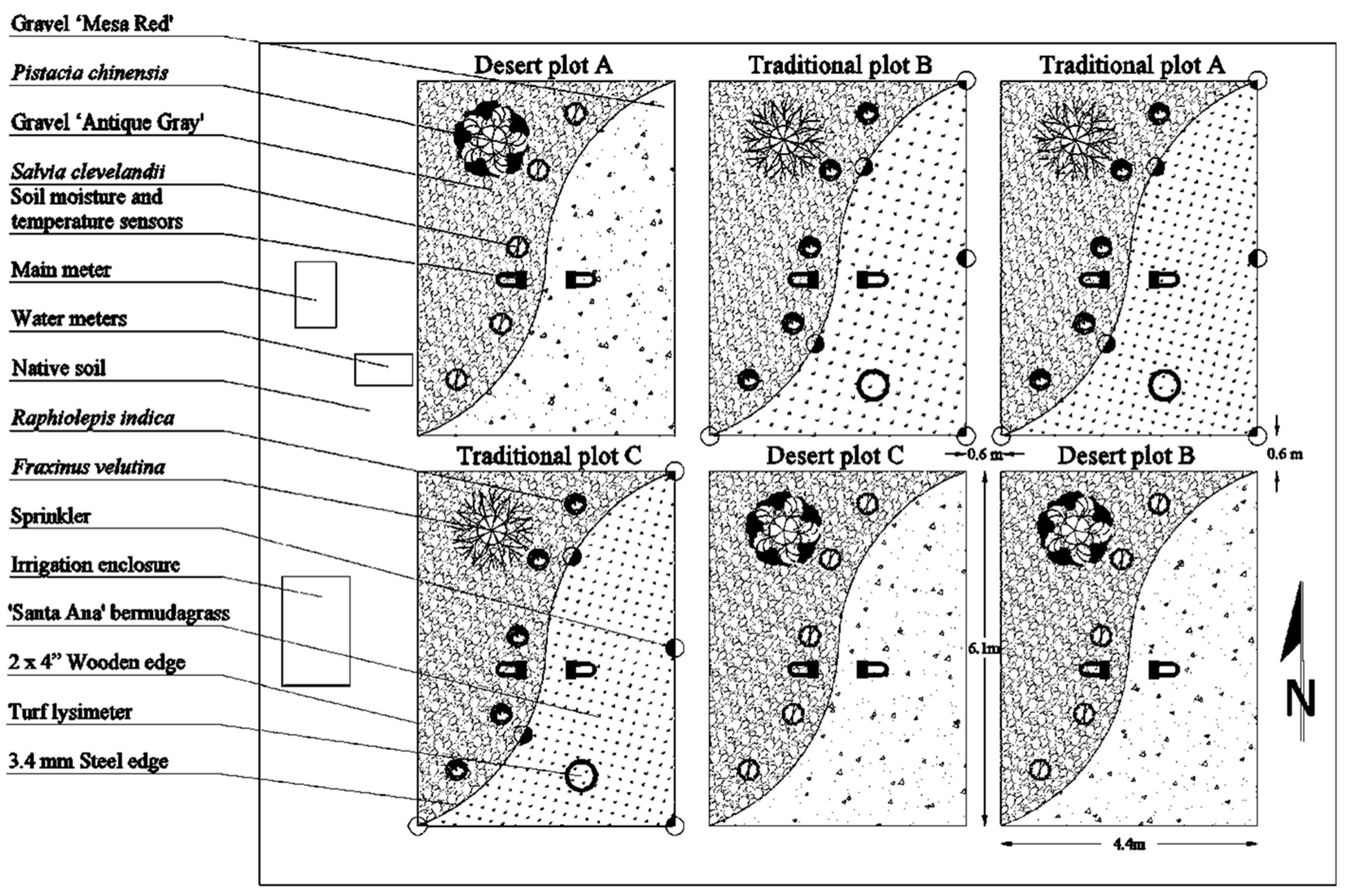
2.1. Location, Landscape Design and Construction

The study was conducted at the Fabian Garcia Science Center (lat. 32°16′45.8″N, long. 106°46′24.7″W, elevation 1183 m) at New Mexico State University in Las Cruces, NM, USA. Las Cruces, located in the Chihuahuan desert, is in USDA Plant Hardiness Zone 8a [14]. Average high temperature is above 30 °C from May to September with average lows of −1.6 °C in December and January [15].

Plants for this study were selected because they are common in the residential landscape plant palette for USDA zone 8a. All can thrive in the desert environment and are readily available from local nurseries. In addition, plants were selected because they had similar water use levels (low to moderate) [16]. Tree species used were 2.5 cm caliper Arizona ash (Fraxinus velutina Torr.) and Chinese pistache (Pistacia chinensis Bunge). Shrub species used were 20 L (5 gal) Indian hawthorn (Rhaphiolepis indica (L.) Lindl) and Cleveland sage (Salvia clevelandii Gray). The desert landscape consisted of one Chinese pistache and five Cleveland sages. The Chinese pistache, while not native to the desert southwest, is drought resistant and often used in arid region landscapes because of its showy fall color and fruits [17]. Cleveland sage, while native to San Diego County CA, USA, performs well in arid regions because it likes well-drained soil and does best when watered weekly or even less often, which allows the soil has time to dry out between waterings [18]. The traditional landscape was composed of one Arizona ash, five Indian hawthorns and bermudagrass. Though called the ‘Arizona’ ash, this tree is in fact native from Texas and northern Mexico west to California and requires monthly deep soakings once established [18] It is commonly included in residential landscapes because of its uniform oval shape [17]. Indian hawthorn is native to China and performs best in moist soils, though can be watered less frequently once established [17]. Bermudagrass was selected for the traditional plots because it is the most adapted warm season grass which performs well in arid areas such as Las Cruces, NM, USA [19].

Six 26.8 m² (6.1 m × 4.4 m) outdoor landscapes were constructed, three containing 13.4 m² (50%) Santa Ana bermudagrass (Cynodon dactylon × C. transvaalensis (L.) Pers. ‘Santa Ana’) and 13.4 m² (50%) antique gray gravel with in-ground container plants (traditional landscape) and three consisting of 13.4 m² mesa red gravel and 13.4 m² antique gray gravel with in-ground container plants (desert landscape). Gravel for each of the landscapes had an average diameter of 1.9 cm and was installed 5.1 cm deep. The landscapes were arranged randomly on the experiment site with one desert and two traditional landscapes to the north, and one traditional and two desert landscapes to the south (Figure 1). Each plot was edged with 5.1 cm × 10.2 cm treated pine and separated from each other with a 5.1 cm antique gray gravel walkway (Figure 1). Native soil in each landscape was Glendale clay loam, a well-drained, deep soil formed in mixed alluvium with a 152 cm root zone [20].

2.2. Plant Materials, Lysimeter Construction, and Evapotranspiration Measurement

Bermudagrass (Gardner Turfgrass, Santa Theresa, NM, USA) plots were sodded in October 2005 and allowed to establish until April 2007 when data collection started. Parker’s Super Soilife Sulfate of Ammonia (21N-0P-0K, 24% S) (Parker Fertilizer, Byer, TX, USA) was applied every two weeks from April to September at a rate of 52 kg·ha⁻¹ of N. The turf was mowed weekly (at 9.5 cm high) with a rotary mower (Yard Machines, Cleveland, OH, USA). Grass clippings were bagged and removed.

We used gravimetric water loss and metrological data to calculate crop coefficients (K_c). According to Allen et al. [21], K_c is computed by dividing crop evapotranspiration (ET_crop) by reference evapotranspiration (ET_o). The daily ET_crop was calculated by measuring plant 24-h gravimetric water loss in cubic centimeters and divided by the total leaf area in square centimeters for that plant [21]. Reference evapotranspiration was collected from Fabian Garcia Science Center’s weather station that was located 15 m east of the plots [22].

Weighing lysimeters, used to measure 24-h water use (ET_crop) for the bermudagrass were installed in turf areas. Within each turf area a 10.2 cm wide × 15.2 cm deep core was cut into turf using a golf hole cup cutter (Par Aide 1001-1, Lino Lakes, MN, USA). Two hours after the turf area was irrigated, the turf core was removed intact from the ground with the golf hole cup cutter and weighed using a top-loading balance (Model QC 60FEG SOUR, Sartorius, Edgewood, NY, USA) to determine its initial weight. The turf was then reinserted into the ground and twenty-hours later, the core was extracted from the turf area and reweighed to determine gravimetric moisture. The core was reinserted into the ground after each measurement.

To facilitate the measurement of 24-h water use, trees and shrubs were installed in an in-ground, pot-in-pot container system that functioned as a weighing lysimeter [23]. This pot-in-pot system uses a socket pot (Classic 8000 Econo-Grip, Nursery Supplies, Orange, CA, USA), permanently sunken in the ground with another pot containing the plant placed inside the socket pot. For drainage, a gravel bed of 5.1 cm of 1.9 cm gravel was placed at the bottom of the hole before the socket pot was installed in the ground. The trees were planted in 57 L (15 gal) plastic container pots and the shrubs in 38 L (10 gal) plastic container pots. All plants were obtained from Sunland Nurseries, Las Cruces, NM, USA and were potted into a growing substrate of 1:1 by volume Canadian sphagnum peat moss (Sun Gro Hort., Bellevue, WA, USA) and perlite (Sun Gro Hort., Bellevue, WA, USA). All plants were fertilized every three months with slow release fertilizer (Osmocote, 15N-22P-13.2K, The Scotts Co., Marysville, OH, USA) at a rate of 28.3 g per pot.

Tree and shrub 24-h moisture loss was determined weekly. The pot with the plant was lifted from the socket plot and placed on the top-loading balance (Model QC 60FEG SOUR). Pot weight was obtained about two hours after an irrigation event (every Tuesday at 8:30 a.m.) and then weighted again 24-h later (every Wednesday at 8:30 a.m.).

2.3. Irrigation System

The irrigation system consisted of one metered main line connected to three individually metered (Hersey 420 Series Composite, Mueller Systems, Cleveland, NC, USA) sprinkler zones and one metered (Hersey 420 Series Composite, Mueller Systems, Cleveland, NC, USA) drip zone. The turf sprinkler-irrigated zones had six pop-up (10.16 cm) spray sprinklers (Van 1800, Rain Bird Corp., Glendora, CA, USA). Due to the informal design of the plots, sprinkler radius of throw and arc was adjusted to prevent overspray into gravel, tree, and shrub areas. Drip irrigation was supplied using a single 1.3 cm metered polyethylene line and 7.6 liter per hour (2 GPH) pressure-compensating emitters (Model SW20, Rain Bird, Azusa, CA, USA). Each tree had four emitters and each shrub had two emitters. Water use data was recorded every Tuesday after the plots were irrigated. Lower quarter distribution uniformity (DU) and net precipitation rates of the sprinkler system averaged 33% and 37.8 mm·h⁻¹, respectively.

2.4. Irrigation Regimes

Plots were irrigated at 50% and 100% ET with irrigation amounts set at the onsite controller using the HydroPoint ET Everywhere^® data. The ET data was wirelessly transmitted to the controller every day using the ET Everywhere^® data service and the ET was calculated using the standard Penman–Montieth equation [24]. A Toro Intelli-Sense Controller (Model TIS-612, Toro, Bloomington, MN, USA), was connected to the irrigation systems, and enabled with HydroPoint ET Everywhere^®, which controlled the irrigation based on ET. Based on preliminary assessment of drip flow rates and sprinkler net precipitation rates, the controller was programmed to irrigate at either 100 or 50% ET between 4:00 AM and 6:30 AM. The controller received daily ET data via the National Weather Service satellite and adjusted irrigation amounts based on the ET data received. Additionally, environmental conditions at site were monitored with a weather station that was adjacent to the plots [22].

All species were exposed to the irrigation regime for the same length of time, but not all physiological measurements were taken at the same time. However, each physiological measurement was taken at the same time for all species. For example, transpiration was taken on the same date for all species, thus allowing the data to be compared. The irrigation regime of the six plots used a modified crossover design to assure proper replication. Throughout the experiment, irrigation occurred every other day. There were a total of six irrigation treatment periods over the course of the experiment. Each treatment period began with an acclimation period, followed by a varying amount of time for data collection, depending upon season (

Table 1. Irrigation table for six research landscape plots, 3 traditional and 3 desert, used to assess water use and performance of plants in contrasting landscapes. Percentages indicate amount of irrigation provided, based on percent of calculated evapotranspiration (ET).

			Traditional Plots			Desert Plots
Treatment	Duration	Data Collection	A	B	C	A	B	C
1 Late Spring/Early Summer	23 April to 16 June 2007 (Weeks 1–8)	3 May to 14 June 2007 (Weeks 2–8)	100%	100%	50%	100%	100%	50%
2 Late Summer	17 June to 11 August 2007 (Weeks 9–16)	5 July to 31 July 2007 (Weeks 11–15)	50%	50%	100%	50%	50%	100%
3 Early Fall	12 August to 6 October 2007 (Weeks 17–24)	12 September to 4 October 2007 (Weeks 21–24)	100%	100%	50%	100%	100%	50%
4 Late Fall	7 October to 24 November 2007 (Weeks 25–31)	25 October to 15 November 2007 (Weeks 27–30)	50%	50%	100%	50%	50%	100%
5 Early Winter	25 November 2007 to 2 Feb. 2008 (Weeks 32–41)	10 January to 31 January 2008 (Weeks 38–41)	100%	100%	50%	100%	100%	50%
6 Late Winter	3 February to 15 March 2008 (Weeks 42–46)	21 February to 6 March 2008 (Weeks 44–46)	50%	50%	100%	50%	50%	100%

).

2.5. Monitoring Soil Moisture and Landscape Surface Temperature

To compare soil moisture and surface and soil temperatures between the two landscapes types, combination temperature probes and soil moisture sensors and surface temperature probes were installed in the middle of the plots in each type of surface within each landscape type in October 2006. Combination soil moisture and soil temperature sensors (GroPoint, Environmental Sensors, Victoria, BC, Canada) were installed 15.2 cm underground in each plot. Sensors were placed in the middle plots and about 15.2 cm from a gravel/gravel or gravel/turf interface. Each combination probe was connected to its own data logger that output temperature and soil moisture through separation ports. A HOBO shuttle (Onset Computer Corp., Bourne, MA, USA) was used to transfer temperature and moisture data from the data loggers to a computer. Surface temperature probes were installed at surface level of the gravel and grass surfaces. Surface temperature probes were connected to data loggers and transferred to a computer via the ONSET shuttle. All data were recorded daily.

2.6. Plant Water Relations

Stem water potential (Ψ_md) at midday was measured once weekly using a pressure chamber (Model 1000, PMS Instruments, Corvallis, OR, USA). For the Indian hawthorn and sage, three different shrubs were randomly selected weekly from each plot. For the Indian hawthorns, a stem with two to five leaves was used in the pressure chamber. A single leaf was used to measure the Ψ_md of the sage. Midday stem water potential of the Chinese pistache and Arizona ash trees were measured on a single terminal leaflet. Leaves chosen were the youngest, fully expanded leaves on each plant. Transpiration and stomatal conductance (g_s) were measured using a steady-state porometer (LI-1600; LI-COR, Lincoln, NE, USA).

2.7. Relative Water Content

Relative water content (RWC) was measured weekly on the youngest, fully expanded leaves. For the Indian hawthorn and sage, three different shrubs were randomly selected weekly, and the three Chinese pistache trees and the three Arizona ash trees were measured weekly. A single leaf was chosen from the Indian hawthorn and two opposite leaves were taken from the Cleveland sages. For the Chinese pistache and Arizona ash, a single terminal leaflet was used.

2.8. Cell Osmolality

Cell osmolality for all shrubs and trees were measured weekly. Three Indian hawthorns and Cleveland sages were randomly selected each week from each plot and three of the youngest, fully expanded leaves were harvested for measurement. Three terminal leaflets from all of the Chinese pistache and Arizona ash trees were also harvested. For Indian hawthorn, Chinese pistache and Arizona ash leaves, 18 discs (each 28 mm²) were removed using a hole punch, while an entire leaf was used for the Cleveland sages. The leaf samples were placed in foil and stored at −20 °C for 24 h and then placed at room temperature (approx. 25 °C) to thaw. Cell sap was extracted from the thawed sample by centrifugation for 60 min at 13,200 rpm (5955.3 g). Cell osmolality was measured using a self-calibrating vapor pressure osmometer (Vapro Model 5520, Wescor, Logan, UT, USA). Cell osmolality was converted to osmotic potential using Van’t Hoff’s equation Ψs = −CiRT where C = concentration of solution as molality (moles per kg of water) moles/kg, i = the ionization constant, R = gas constant (0.00831 kg MPa·mol⁻¹·k⁻¹) and T = temperature (K).

2.9. Data Analysis

The analysis was based on a crossover experiment because there was more than one treatment or irrigation level [25]. No carryover effects were assumed because of the limit in landscape plots and the two-week acclimation period at the start of each treatment for the individual plants and turf areas. Data were analyzed based on a model with fixed and random effects using the mixed-model procedure in SAS^® software, version 9.1 (SAS Inst., Cary, NC, USA). Stem water potential at midday, transpiration, g_s, relative water content and cell osmolality of plants were analyzed separately by species. Temperature and soil moisture of bermudagrass, gray and mesa red gravel also were analyzed using a mixed model. The mixed models accounted for missing data and included fixed effects for irrigation treatments, season, bermudagrass or gravel type, week within seasons, treatment by season and treatment by week within season effects. The mixed models also incorporated random effects for the landscape plots, plot by season, plot by week within season and the individual plant. The Kenward–Rogers ddfm option was used to calculate denominator degrees of freedom; least square means for significant effects were compared using the pdiff option and plotted for graphs [26]. Significance was defined for p < 0.05.

3. Results and Discussion

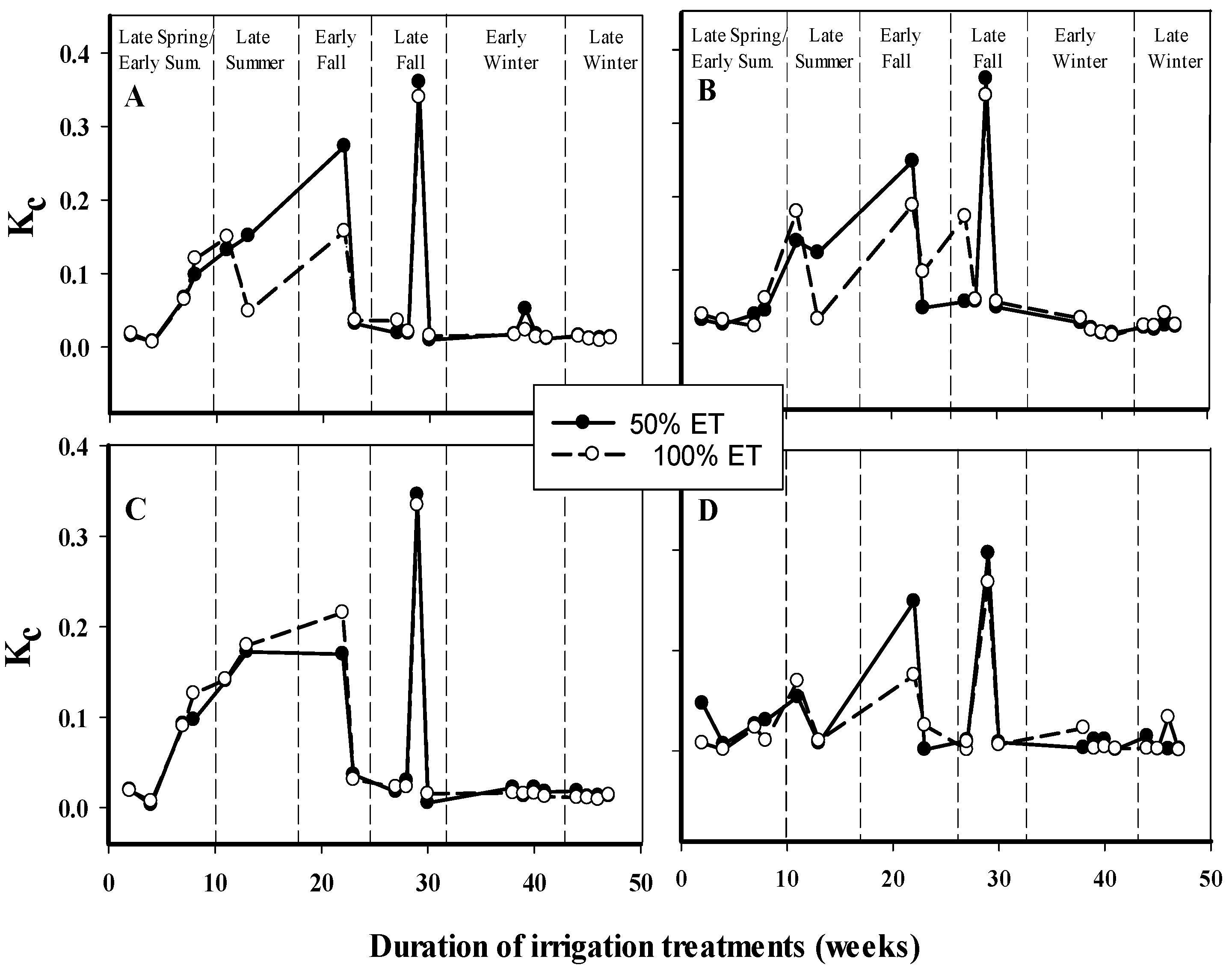
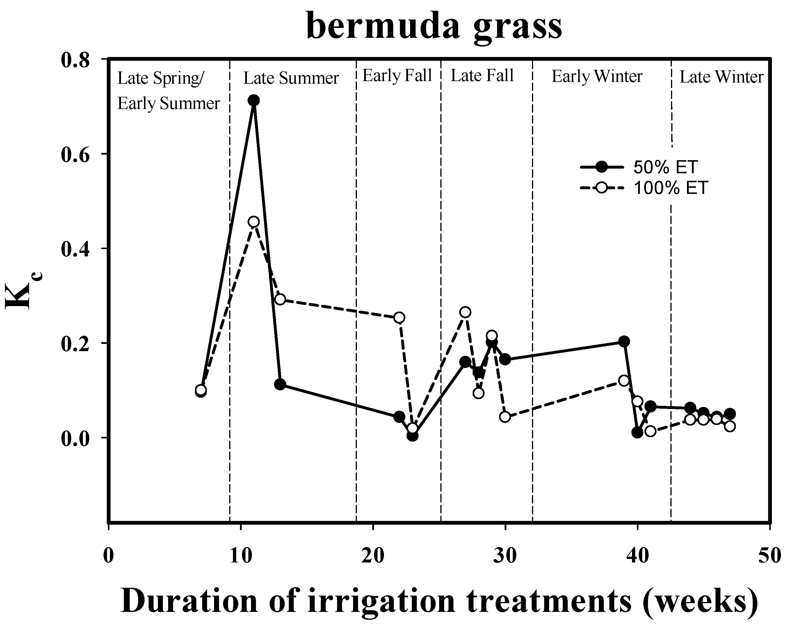
3.1. Crop Coefficients

The K_c of Indian hawthorn (Figure 2A), Cleveland sage (Figure 2B), Arizona ash (Figure 2C) and Chinese pistache (Figure 2D) had greater values in late fall (October–November) than in other seasons. Mature citrus trees have shown higher K_c values in fall than in summer and maximum values in winter [27]. So, the increase in K_c we observed is consistent with the Petillo study [27]. However, the spikes in K_c observed during our study in late fall cannot be attributed to analogous spikes in temperature. Other atmospheric effects that have been shown to impact K_c, such as air vapor density, wind speed or solar radiation [28] may have caused these spikes. As expected, the K_c of trees and shrubs decreased during winter (January–early March) (Figure 2A–D), when ambient temperature decreases, and plant transpiration and water uptake slow. Schuch and Burger [11] have assessed the K_c values of above ground container plants and questioned the reliability of those K_c values because container plants do not meet the specific conditions used to determine K_c. While plants in our in-ground container system approximated field conditions better than above ground container plants, nevertheless, our K_c values must be viewed with caution. First, K_c values are derived from above ground container plants. Second, the irrigation treatments applied reduced water to some plants, thus violating the non-stressed condition that is relevant to derive K_c values. What the K_c values show is that period from 16 June to 24 November encompass a critical period for water conservation for irrigated trees and shrubs.

The K_c for bermudagrass was highest during late summer (Figure 3). Bermudagrass was irrigated at 100% ET daily with an average summer K_c of 0.80 [29], which is greater than our summertime K_c high value (0.71) for grass irrigated at 50% ET. While we attribute the difference in K_c (0.09) of bermudagrass in their study [29] to differences in irrigation, the higher late summer K_c value of grass irrigated at 50% ET warrants further investigation. Overall, K_c values were lower for grass irrigated at 50% ET. Thus, the change in irrigation amount from 100% to 50% ET offers promise for water conservation because of reduced water use when compared to that of turf irrigated at 100% ET. Although the two-week acclimation period that was provided for the turf assumes no carry over effect of the previous irrigation regime, it is possible the turf may have acclimated to reduced moisture regime by curtailing water use.

During the winter season of our study, K_c for the bermudagrass ranged from 0.20 to <0.01 for turf irrigated at 50% ET. While Garrot and Mancino [30] showed that K_c values of bermudagrass dropped during late fall and early winter, it is clear from this study that the turf irrigated at 50% ET show reduced water use. Furthermore, we did not observe any visual differences in turf quality during the experimental period.

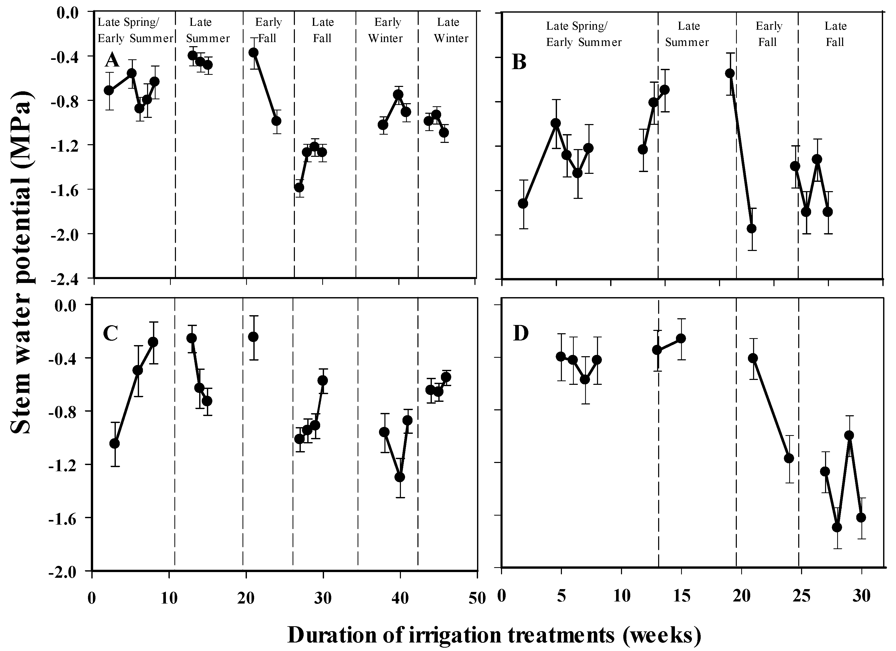
3.2. Stem Water Potential

There were only seasonal differences in stem water potential (Ψ_md) for Indian hawthorn (p = 0.0006), Arizona ash (p = 0.0081), cleveland sage (p < 0.0001) and Chinese pistache (p = 0.0002) (Figure 4A–D). Chinese pistache Ψ_md remained stable going from late spring/early summer irrigation through late summer. This stability in Ψ_md indicated that Chinese pistache was able to recover and rehydrate after changes in irrigation treatments and these irrigation changes did not have an impact on pistache during the hotter seasons. The Ψ_md values of Chinese pistache from late spring to late summer were consistent with that of Pour et al. [31], where Chinese pistache had similar leaf water potential (−0.33 to −0.4 MPa), regardless of irrigation regime.

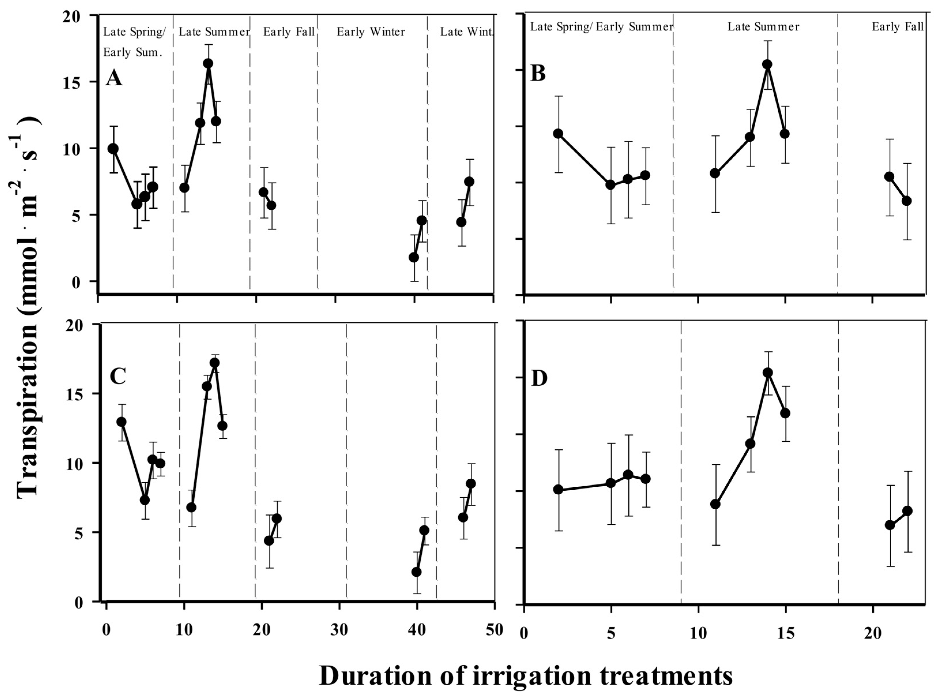
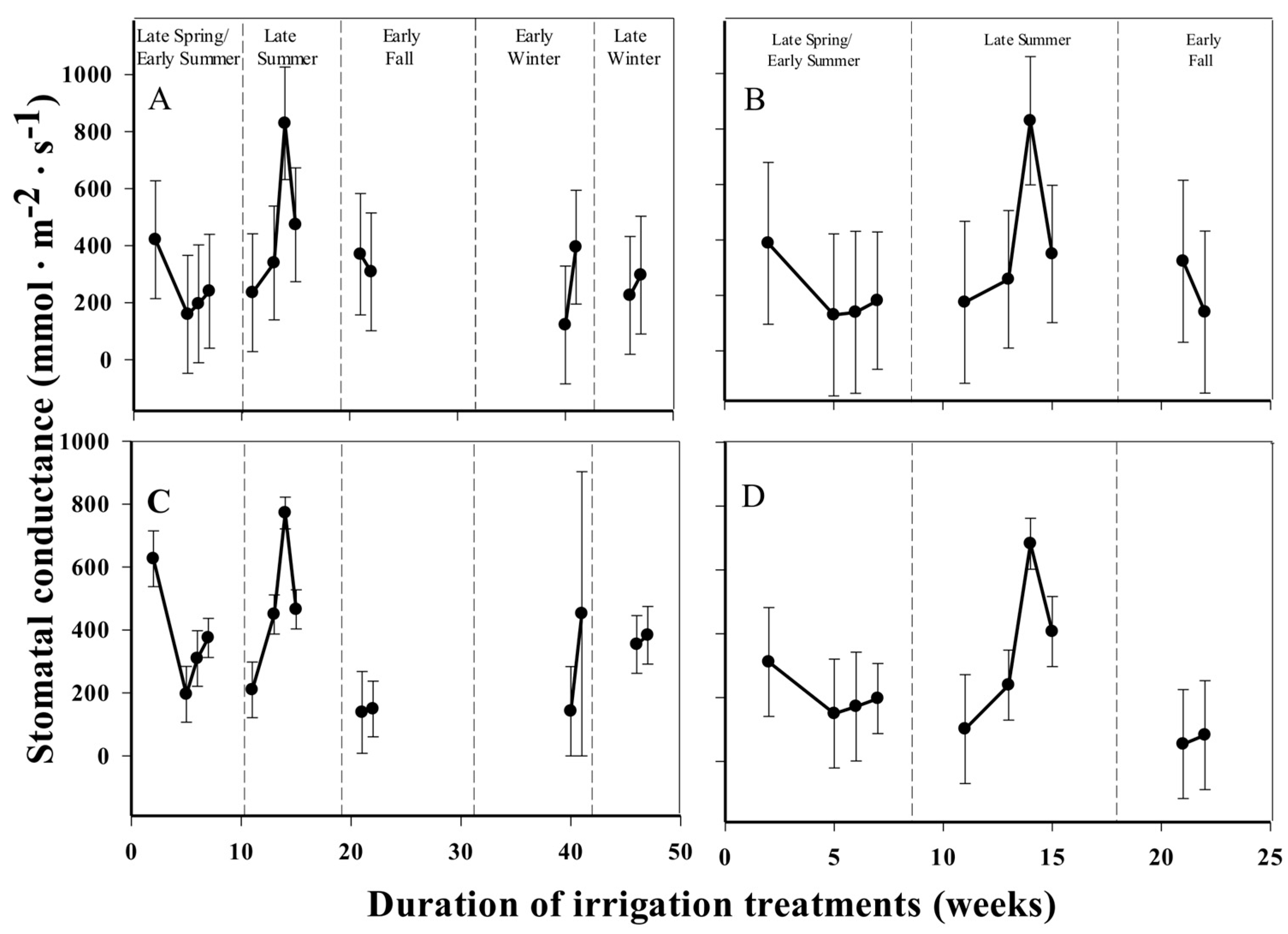
3.3. Transpiration and Stomatal Conductance

All four species showed greater transpiration (Figure 5A–D) and g_s (Figure 6A–D) during warmer seasons, regardless of irrigation regime. This is to be expected as it is normal for summer days to have intense daytime temperatures, resulting in an increase in evaporative water loss from leaves. As temperatures declined in fall and early winter seasons, so did plant transpiration and g_s.

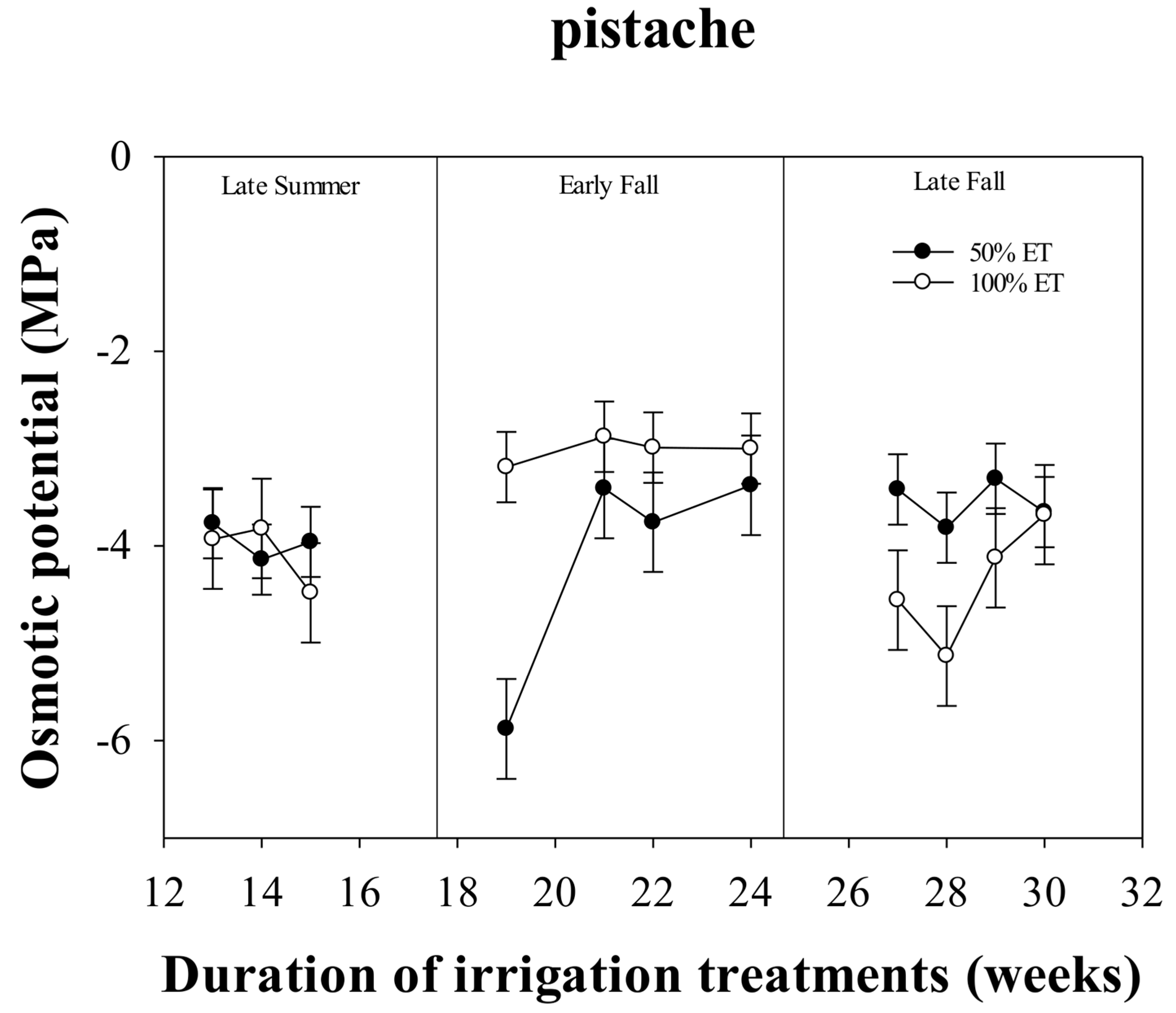
3.4. Osmotic Potential

For Indian hawthorn, Cleveland sage and Arizona ash, there were no significant differences in osmotic potential for plants irrigated at either 50 or 100% ET during each season or within weeks in a season (data not shown). During early fall, average osmotic potential of Chinese pistache plants irrigated at 50% ET was lower (−4.12 MPa) than those irrigated at 100% ET (−3.01 MPa) (Figure 7). When plants receiving irrigation treatment at 50% ET were increased to 100% ET at the end of late fall, osmotic potential of Chinese pistache became less negative (−3.7 MPa). Although irrigating Chinese pistache plants at 50% may have stressed them in early fall, decreased negativity in osmotic potential indicates that the plants were able to rehydrate because of the increased ability to extract more water from the cell as solutes in the cell increased [32].

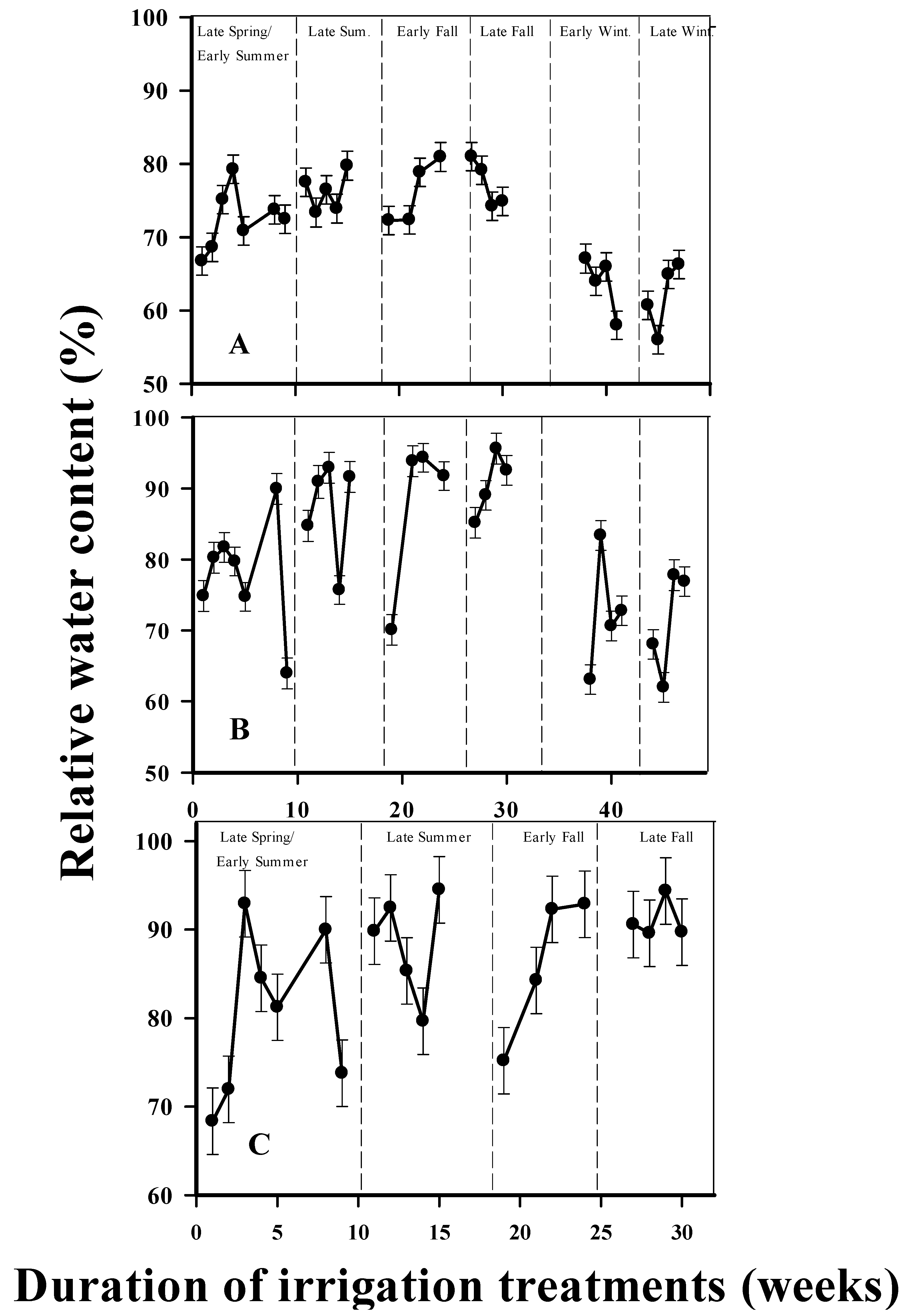
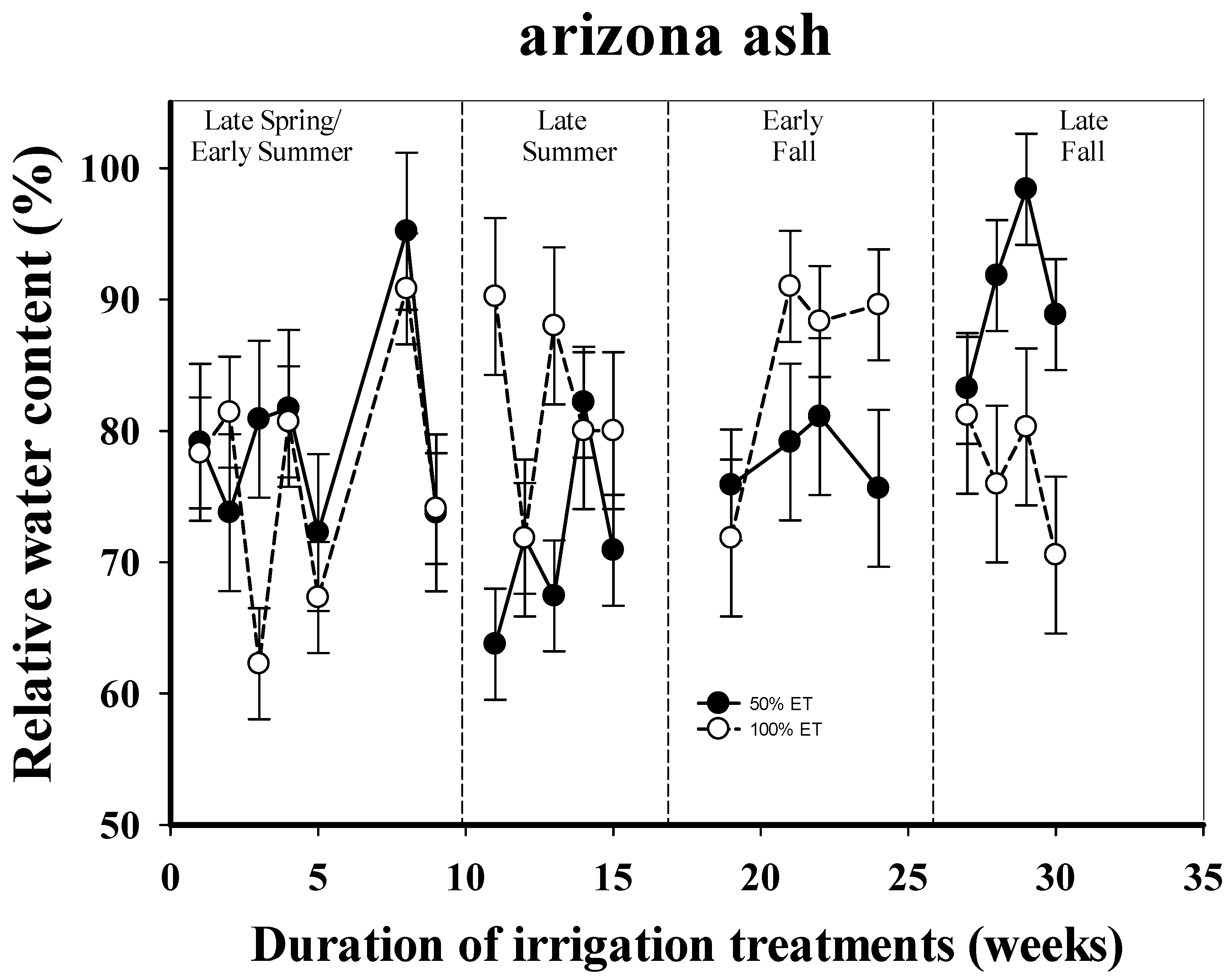
3.5. Relative Water Content

When weeks in a season were compared to other weeks in a different season, there was a difference in RWC for Indian hawthorn (p = 0.0002), Cleveland sage (p < 0.0001), and Chinese pistache (p = 0.0002) (Figure 8A–C). Arizona ash (Figure 9) showed changes (p = 0.0003) in the relative water content when irrigation treatment was reduced from 100% ET in early fall to 50% ET in late fall. In early fall, Arizona ash irrigated at 50% ET had a RWC of 79%, which was lower than the 91% RWC of plants irrigated at 100% ET. The decreased irrigation at 50% ET in early fall may have caused the solute accumulation in response to drought. This adjustment in osmotic cell contents might have allowed Arizona ash to maintain a high RWC during the acclimation period after increasing irrigation treatment levels from 50% to 100% ET. By late fall, RWC of Arizona ash rapidly declined showing the short term and reversible effect of osmotic adjustment. This short-term effect may be attributed to the rapid change in irrigation regimes. Also, this shows that osmotic adjustment is only a temporal drought adaptation mechanism when drought occurs rapidly [32].

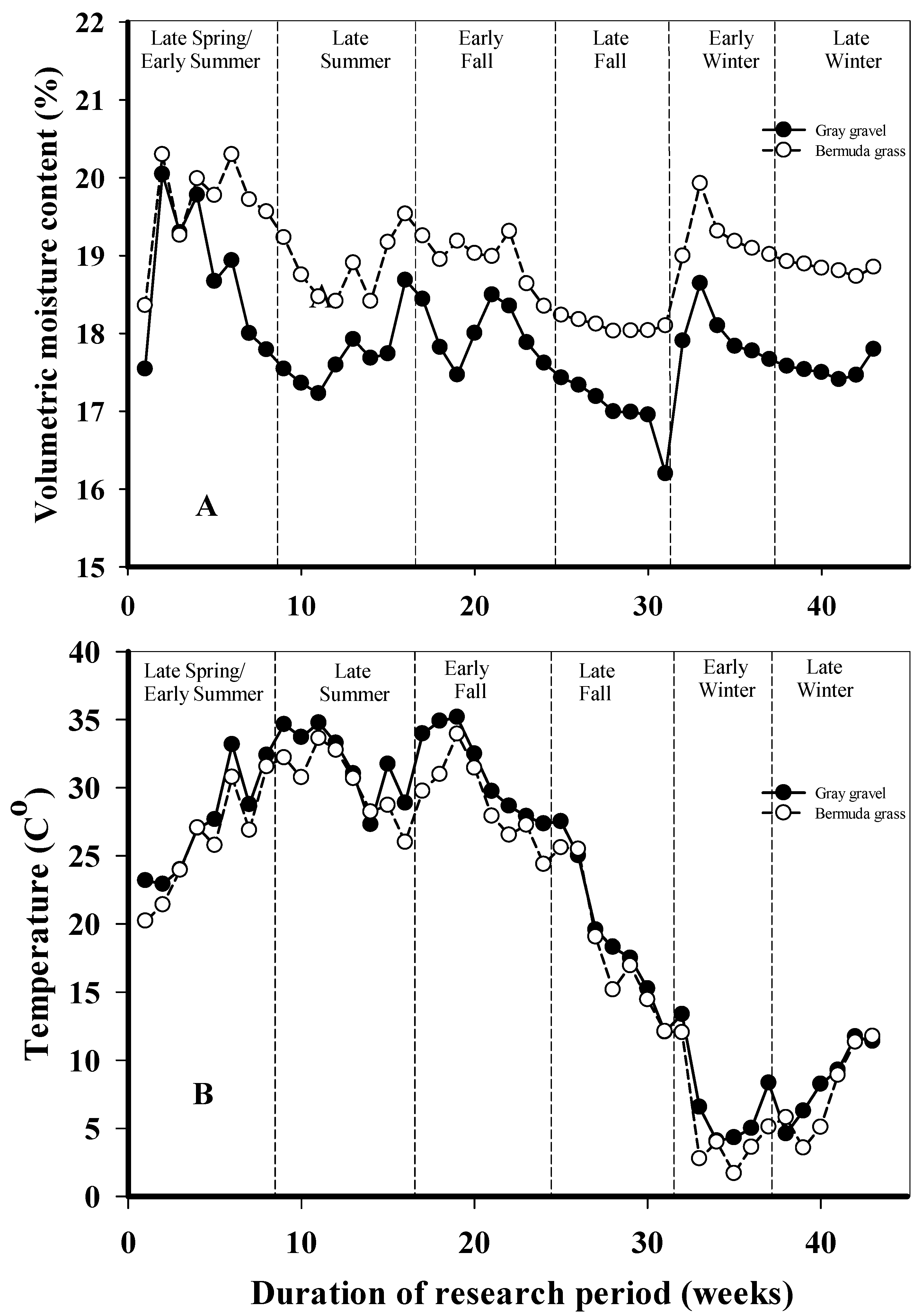
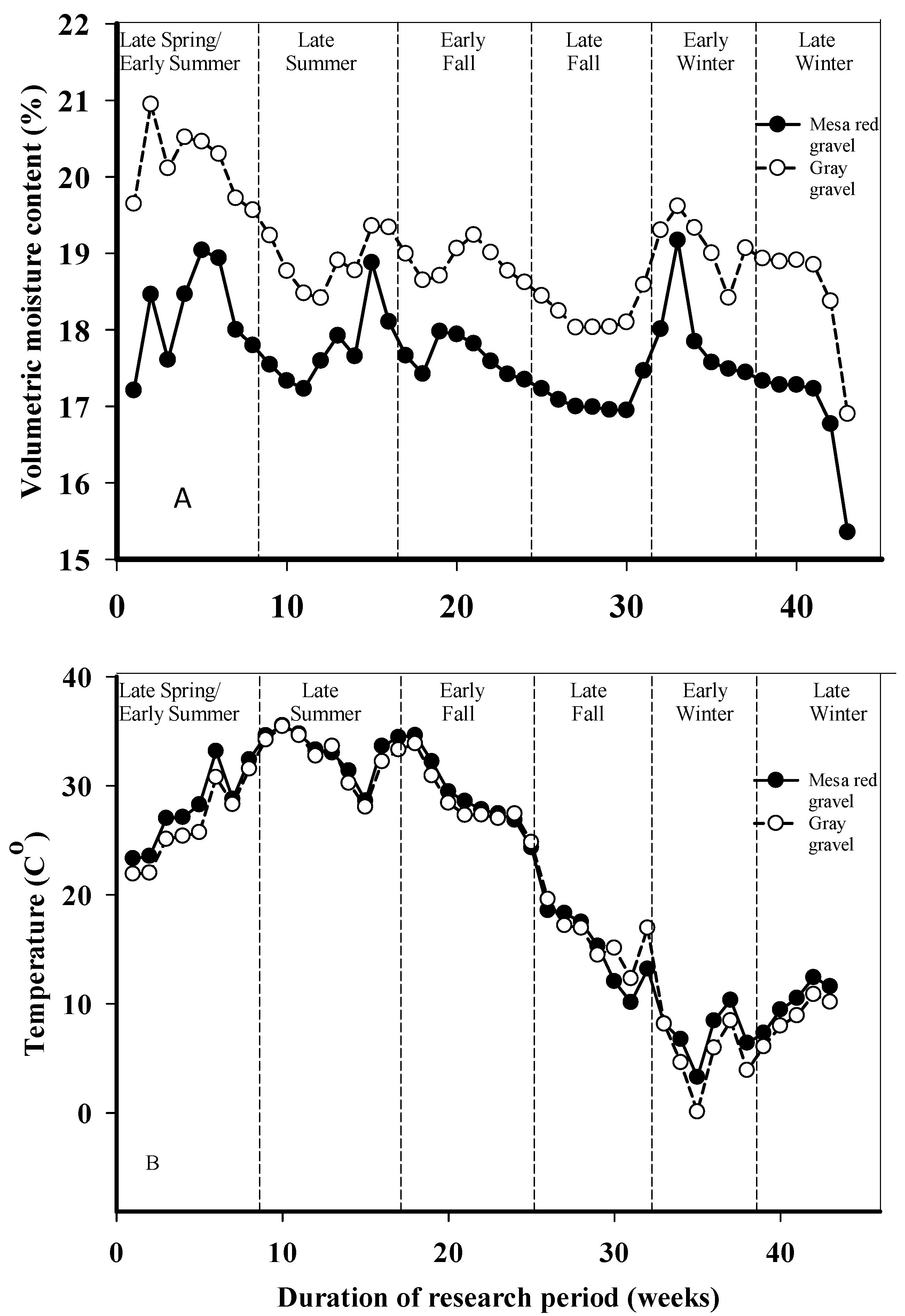
3.6. Volumetric Soil Moisture and Temperature

In the traditional plots, soil 15.2 cm underneath the bermudagrass had a higher moisture content (19%) than that of the soil under the gray gravel (18%) (p < 0.0001) (Figure 10A). This difference in soil moisture content could be explained by the fact that bermudagrass was sprinkler irrigated.

In the traditional plots, bermudagrass and gray gravel showed seasonal differences in temperature (p < 0.0001), with the highest temperatures during the hotter seasons from late spring to early fall, and declined in the cooler seasons (Figure 10B). These seasonal differences in temperature could serve as drivers for changes in physiological parameters such as Ψ_md, g_s, and transpiration. For traditional plots, there was a difference (p = 0.0026) in temperature, with bermudagrass averaging about 16.4 °C and gray gravel averaging 19 °C. Higher temperatures for gray gravel may indicate the increased heat load of gravel versus turfgrass.

In the desert plots, soil moisture under gray gravel averaged about 19% (p < 0.0001), which was statistically different from that of mesa red gravel which averaged 18% (Figure 11A). We attribute this difference in soil moisture between gray gravel and mesa red gravel to the fact that plants were planted and irrigated within the gray gravel and not in the mesa red.

Seasonal differences in temperature (p < 0.0001) were shown between the gray and mesa red gravel. High temperatures for both gravel types were detected during late spring to early fall, and drops in temperature from late fall to late winter (Figure 11B). The lack of overall temperature differences between gravel types might indicate that gravel type is not a matter of concern for water conservation.

3.7. Overall Water Applied

The total water use for the entire research period was 7820 L for traditional plots and 3230 L for the desert plots (data not shown). The traditional plot water use was based on the specific tree and shrub species, as well as the bermudagrass, while the desert plot water use is based on the chosen trees and shrubs. The driver of greater water use in the traditional plots seems to be mainly a function of overall vegetated area.

4. Conclusions

This research demonstrates that the selected plants can maintain adequate physiological performance well when irrigated for periods at 50% ET. Furthermore, it is evident that drought tolerant plants irrigated at 100% ET also will use the applied water. The Indian hawthorn from the traditional plot and the Cleveland sage from the desert plot had similar physiological responses to irrigation reduction. Neither Indian hawthorns nor Cleveland sages showed any differences when irrigation amounts were changed, which indicates that both shrubs were able to thrive under reduced irrigation for a limited time without showing significant negative physiological effects. In the case of these two shrubs, employing a reduced irrigation regime for short intervals might be a strategy that home owners could use to conserve water. The results also imply that for all four plant species, it is possible that irrigation could be reduced to 50% ET during certain intervals throughout the year and later increased to full irrigation without any negative impacts on physiological health. Since the traditional plots had the larger vegetated surface area because of the bermudagrass, we attribute the difference in total water applied to the larger vegetated surface.

This research implies that homeowners could bolster their water conservations strategies by adopting a watering regime for shrubs that includes short periods (up to four weeks) of reduced irrigation without affecting the health of the plants. With water usage for even small plots with turf more than twice that of desert plots, home owners and landscape managers that change to larger areas of trees and shrubs in place of turfgrass could realize substantial increases in water conservation.

References

1. Spinti, J.E.; St. Hilaire, R.; VanLeeuwen, D. Balancing landscape preferences and water conservation in a desert community. HortTechnology 2004, 14, 72–77. [Google Scholar]
2. Spinti, J.E. Balancing Landscape Preferences and Water Use in a Desert Environment. Master’s Thesis, New Mexico State University, Las Cruces, NM, USA, 2002. [Google Scholar]
3. Al-Ajlouni, M.G.; VanLeeuwen, D.; St. Hilaire, R. Linking urban residential landscape types in a desert environment to landscape water budgets. HortTechnology 2014, 24, 307–312. [Google Scholar]
4. Home Irrigation and Landscape Combinations for Water Conservation in Florida. Available online: http://edis.ifas.ufl.edu/ae287 (accessed on 12 January 2018).
5. Sovocool, K.A.; Morgan, M.; Bennett, D. An in-depth investigation of xeriscape as a water conservation measure. J. Am. Water Works Assoc. 2006, 98, 82–93. [Google Scholar] [CrossRef]
6. St. Hilaire, R.; Arnold, M.A.; Wilkerson, D.C.; Devitt, D.A.; Hurd, B.H.; Lesikar, B.J.; Lohr, V.I.; Martin, C.A.; McDonald, G.V.; Morris, R.L. Efficient water use in residential urban landscapes. HortScience 2008, 43, 2081–2092. [Google Scholar]
7. Pittenger, D.R.; Shaw, D.A.; Hodel, D.R.; Holt, D.B. Responses of landscape groundcovers to minimum irrigation. J. Environ. Hortic. 2001, 19, 78–84. [Google Scholar]
8. Staats, D.; Klett, J.E. Water conservation potential and quality of non-turf groundcovers versus Kentucky bluegrass under increasing levels of drought stress. J. Environ. Hortic. 1995, 13, 181–185. [Google Scholar]
9. Shackel, K. A plant-based approach to deficit irrigation in trees and vines. HortScience 2011, 46, 173–177. [Google Scholar]
10. Feser, C.; St. Hilaire, R.; VanLeeuwen, D. Development of in-ground container plants of Mexican elders exposed to drought. HortScience 2005, 40, 446–450. [Google Scholar]
11. Schuch, U.K.; Burger, D.W. Water use and crop coefficients of woody ornamentals in containers. J. Am. Soc. Hortic. Sci. 1997, 122, 727–734. [Google Scholar]
12. Thayer, R. Public response to water-conserving landscapes. HortScience 1982, 17, 562–565. [Google Scholar]
13. Lockett, L.; Montague, T.; McKenney, C.; Auld, D. Assessing public opinion on water conservation and water conserving landscapes in the semiarid southwestern United States. HortTechnology 2002, 12, 392–396. [Google Scholar]
14. Plant Hardiness Zone Map for the United States. Available online: http://planthardiness.ars.usda.gov/PHZMWeb/ (accessed on 1 February 2018).
15. U.S. Climate Data. Available online: http://www.usclimatedata.com/climate/las-cruce/new-mexico/united-states/usnm0492/2017/1 (accessed on 1 February 2018).
16. A Guide to Estimating Irrigation Water Needs of Landscape Plantings in California: The Landscape Coefficient Method and WUCOLS III. Available online: http://www.water.ca.gov/wateruseefficiency/docs/wucols00.pdf (accessed on 14 December 2017).
17. St. Hilaire, R. Landscape Plants for the Lower Rio Grande Basin; New Mexico State University: Las Cruces, NM, USA, 2012; pp. 20, 207 & 265. [Google Scholar]
18. Jones, W.D.; Sacamano, C.M. Landscape Plants for Dry Regions: More than 600 Species from Around the World; De Capo Press: Boston, MA, USA, 2000; pp. 170 & 291. [Google Scholar]
19. Christians, N.E.; Patton, A.J.; Law, Q.D. Fundamentals of Turfgrass Management; John Wiley & Sons: Hoboken, NJ, USA, 2016. [Google Scholar]
20. USDA Soil Conservation Service. Soil Survey of Dona Ana County Area, New Mexico. Available online: https://www.nrcs.usda.gov/Internet/FSE_MANUSCRIPTS/new_mexico/NM690/0/nm_dona_ana.pdf (accessed on 16 January 2018).
21. Allen, R.G.; Pereira, L.S.; Smith, M.; Raes, D.; Wright, J.L. FAO-56 dual crop coefficient method for estimating evaporation from soil and application extensions. J. Irrig. Drain. Eng. 2005, 131, 2–13. [Google Scholar] [CrossRef]
22. New Mexico State University. GDD and ET Data for Fabian Garcia SC; NM Climate Center: Las Cruces, NM, USA, 2008; Available online: https://weather.nmsu.edu/ (accessed on 25 September 2017).
23. St. Hilaire, R.; Feser, C.F.; Sammis, T.W.; St. Hilaire, A.S. A system to measure evapotranspiration of in-ground container plants of Mexican elder. HortTechnology 2003, 13, 185–189. [Google Scholar]
24. Snyder, R.L.; Eching, S. Penman-Monteith Daily (24-hour) Reference Evapotranspiration Equations for Estimating ETo, ETr and HS ETo with Daily Data; Regents of the University of California: Oakland, CA, USA, 2002; Available online: http://biomet.ucdavis.edu/Evapotranspiration/PMdayXLS/PMdayDoc.pdf (accessed on 5 February 2018).
25. Kuehl, R.O. Statistical Principles of Research Design and Analysis, 1st ed.; Wadsworth: Duxbury, MA, USA, 1994. [Google Scholar]
26. Kenward, M.G.; Roger, J.H. Small sample inference for fixed effects from restricted maximum likelihood. Biometrics 1997, 983–997. [Google Scholar] [CrossRef]
27. Petillo, M.G.; Castel, J. Water balance and crop coefficient estimation of a citrus orchard in Uruguay. Span. J. Agric. Res. 2007, 5, 232–243. [Google Scholar] [CrossRef]
28. Annandale, J.; Stockle, C. Fluctuation of crop evapotranspiration coefficients with weather: A sensitivity analysis. Irrig. Sci. 1994, 15, 1–7. [Google Scholar] [CrossRef]
29. Brown, P.W.; Mancino, C.F.; Young, M.H.; Thompson, T.L.; Wierenga, P.J.; Kopec, D.M. Penman Monteith. Crop coefficients for use with desert turf systems. Crop Sci. 2001, 41, 1197–1206. [Google Scholar] [CrossRef]
30. Garrot, D.; Mancino, C. Consumptive water use of three intensively managed bermudagrasses growing under arid conditions. Crop Sci. 1994, 34, 215–221. [Google Scholar] [CrossRef]
31. Pour, A.T.; Sepaskhah, A.R.; Maftoun, M. Plant water relations and seedling growth of three pistachio cultivars as influenced by irrigation frequency and applied potassium. J. Plant Nutr. 2005, 28, 1413–1425. [Google Scholar] [CrossRef]
32. Blum, A. Crop responses to drought and the interpretation of adaptation. Plant Growth Regul. 1996, 20, 135–148. [Google Scholar] [CrossRef]
Figure 1. Diagram of six research landscape plots used to assess water use and performance of plants in contrasting landscapes (not to scale).
Sustainability 10 00624 g001
Figure 2. Crop coefficients (Kc) of Indian hawthorn (A), Cleveland sage (B), Arizona ash (C) and Chinese pistache (D), irrigated at 50 or 100% ET. Late spring/early summer was from 23 April to 16 June 2007. Late summer was from 17 June to 11 August 2007. Early fall was from 12 August to 6 October 2007. Late fall was from 7 October to 24 November 2007. Early winter was from 25 November 2007 to 2 February 2008. Late winter was from 3 February to 15 March 2008.
Sustainability 10 00624 g002
Figure 3. Crop coefficients (Kc) of bermudagrass, irrigated at 50 or 100% ET. Late spring/early summer was from 23 April to 16 June 2007. Late summer was from 17 June to 11 August 2007. Early fall was from 12 August to 6 October 2007. Late fall was from 7 October to 24 November 2007. Early winter was from 25 November 2007 to 2 February 2008. Late winter was from 3 February to 15 March 2008.
Sustainability 10 00624 g003
Figure 4. Stem water potentials for Indian hawthorn (A), Arizona ash (B), Cleveland sage (C), and Chinese pistache (D). Bars represent one standard error. Late spring/early summer was from 23 April to 16 June 2007. Late summer was from 17 June to 11 August 2007. Early fall was from 12 August to 6 October 2007. Late fall was from 7 October to 24 November 2007. Early winter was from 25 November 2007 to 2 February 2008. Late winter was from 3 February to 15 March 2008.
Sustainability 10 00624 g004
Figure 5. Transpiration rates for Indian hawthorn (A), Arizona ash (B), Cleveland sage (C), and Chinese pistache (D). Bars represent one stand error. Late spring/early summer was from 23 April to 16 June 2007. Late summer was from 17 June to 11 August 2007. Early fall was from 12 August to 6 October 2007. Early winter was from 25 November 2007 to 2 February 2008. Late winter was from 3 February to 15 March 2008.
Sustainability 10 00624 g005
Figure 6. Stomatal conductance of Indian hawthorn (A), Arizona ash (B), Cleveland sage (C), and Chinese pistache (D). Bars represent one standard error. Late spring/early summer was from 23 April to 16 June 2007. Late summer was from 17 June to 11 August 2007. Early fall was from 12 August to 6 October 2007. Early winter was from 25 November 2007 to 2 February 2008. Late winter was from 3 February to 15 March 2008.
Sustainability 10 00624 g006
Figure 7. Osmotic potential for Chinese pistache. Bars represent one standard error. Late summer was from 17 June to 11 August 2007. Early fall was from 12 August to 6 October 2007. Late fall was from 7 October to 24 November 2007.
Sustainability 10 00624 g007
Figure 8. Relative water content of Indian hawthorn (A), Cleveland sage (B), and Chinese pistache (C). Bars represent one standard error. Late spring/early summer was from 23 April to 16 June 2007. Late summer was from 17 June to 11 August 2007. Early fall was from 12 August to 6 October 2007. Late fall was from 7 October to 24 November 2007. Early winter was from 25 November 2007 to 2 February 2008. Late winter was from 3 February to 15 March 2008.
Sustainability 10 00624 g008
Figure 9. Relative water content of Arizona ash irrigated at 50 or 100% ET. Bars represent one standard error. Late spring/early summer was from 23 April to 16 June 2007. Late summer was from 17 June to 11 August 2007. Early fall was from 12 August to 6 October 2007. Late fall was from 7 October to 24 November 2007.
Sustainability 10 00624 g009
Figure 10. Weekly averaged volumetric moisture content (A) and temperature (B) from data logger for traditional plots. Late spring/early summer was from 23 April to 16 June 2007. Late summer was from 17 June to 11 August 2007. Early fall was from 12 August to 6 October 2007. Late fall was from 7 October to 24 November 2007. Early winter was from 25 November 2007 to 2 February 2008. Late winter was from 3 February to 15 March 2008.
Sustainability 10 00624 g010
Figure 11. Weekly averaged volumetric moisture content (A) and temperature (B) from data logger for desert plots. Late spring/early summer was from 23 April to 16 June 2007. Late summer was from 17 June to 11 August 2007. Early fall was from 12 August to 6 October 2007. Late fall was from 7 October to 24 November 2007. Early winter was from 25 November 2007 to 2 February 2008. Late winter was from 3 February to 15 March 2008.
Sustainability 10 00624 g011