Population Agglomeration and Residential Energy Consumption: Evidence from Japan

Abstract

In the Japanese economy facing environmental restrictions, both the control of greenhouse gas emissions and the boost of regional economic growth are important policy issues. In this context, this study employs econometric methods to investigate whether population agglomeration, which is a potential source of economic growth, contributes to the reduction of energy consumption in the residential sector. The results of the analysis highlight that population agglomeration affects savings in energy consumption. Specifically, over the considered observation period, population agglomeration has saved energy consumption in large metropolitan areas. In contrast, in rural areas, population dispersion has had the opposite effect.

1. Introduction

The changes in Japanese social structure towards adopting a lifestyle based on convenience and comfort parallels the growth in the number of households among the residential consumers in Japan. The trends of high consumption and increasing number of households influences residential energy consumption in Japan (Otsuka [1]). The energy consumption in the residential sector in Japan in 2011 fiscal year, influenced by the energy intensity (i.e., energy consumption per capita), increased more than twice its value to 208.9 as compared to 100 in the 1973 fiscal year. Looking at this trend, it emerges that the energy efficiency of consumer electronic devices improved significantly, and thus the rate of increase in consumption itself slowed down. Nevertheless, as a result of the growth in size and diversification of consumer electronic devices, total energy consumption has been experiencing on an upward trend. The question of how energy consumption can be saved to make it exceed the spread of consumer electronic devices has become a policy issue in Japan.

From the perspective of regional policy, spatial population concentration is cited as a possible solution to this problem. The existence of multiple dwelling housing is more common and widespread in regions where the population is agglomerating as compared to regions where the population is more diffused. In contrast to single dwelling housing, the energy usage in multiple dwelling housing is more efficient because, in the latter case, the housing floor space is generally smaller. Multi-dwelling houses are highly heat-insulating structures and very efficient in cooling and heating. Therefore, it is expected that energy consumption wastage will be reduced. Moreover, in densely populated cities, it is assumed that there will be more opportunities to share the use of electricity, such as for electric lights. In addition, there will be a well-developed public transportation system and thus fewer opportunities to use private cars, resulting in a decrease in energy consumption. All of these factors will contribute to save energy consumption.

Many previous studies have shown that high population density is a driver of energy consumption (Newman and Kenworthy [2], Lariviere and Lafrance [3], O’Neill and Chen [4], Bento and Cropper [5], Liddle [6], Brownstine and Golob [7], Karathodorou et al. [8]). Otsuka and Goto [9] have empirically demonstrated that urban population concentration fosters energy efficiency. Japan’s national land planning has stressed the importance of compact cities from both the economic and the environmental point of view. In this respect, it is important to verify whether compact city policies, which aim for a shift from dispersed to concentrated cities, are effective in enhancing energy savings in the residential sector. Achieving regional economic growth in parallel with limiting greenhouse gas emissions by improving energy efficiency is an important policy issue for the entire Japanese economy. The government has been introducing various policies aimed to reduce greenhouse gas emissions, including green innovation and renewable energy technology diffusion. In recent years, the highly debated climate change problem has worsened in a way that cannot be dealt with by individual elemental technologies. To realize a low-carbon society, Japan should also promote the creation of urban areas, such as compact cities, through urban regional policies, including new system designs, new regulations, and deregulation.

It is in this direction that this study aims to provide empirical evidence on these policy issues. Specifically, regional data on Japan are considered to analyze the effects that population agglomeration, which is the driving force behind the realization of sustainable growth in regional economies, have on energy saving. Empirical research on this topic has already been carried out by Otsuka and Goto [10]. They take an aggregate approach to mainly focus on the impact of population density on the regional total energy. On the contrary, this study highlights the impact in an end-use sector, thus extending the previous study. Specifically, this study intends to clarify the effects of population agglomeration on energy consumption in the residential sector. In Japan, energy efficiency in the residential sector has been worsening (Agency for Natural Resources and Energy, 2016). To improve the energy efficiency of the country as a whole, it is necessary to stop the worsening effect in the residential sector. Thus, this study focuses on the effects of population agglomeration, which is considered a key factor behind energy consumption savings, and shows empirical evidence in support of desirable urban and regional policies.

The analysis framework of this paper follows the one by Otsuka and Goto [10]. Specifically, the dynamic panel model allows to simultaneously capture both static and dynamic effects on the energy consumption of population agglomeration. Moreover, panel data increase the number of observations and allow for both cross-sectional and time changes. Compared to the static model, the dynamic model makes it possible to estimate both short-run (short-run elasticity) and long-run effects (long-run elasticity) of population agglomeration on energy consumption. Specifically, by ascertaining the long-run effects, it is possible to evaluate the impact of population agglomeration on the yearly changes in energy consumption.

The remainder of this paper is as follows. Section 2 illustrates the method for the empirical analysis and the data. Section 3 presents the results. Section 4 concludes the study.

2. Methods

2.1. The Determinants of Energy Consumption

This study focuses on energy consumption (EC) in the residential sector. The residential sector’s EC is defined as the final energy consumption per household.

The objective of this study is to evaluate, based on end use, the effectiveness of population agglomeration as a likely determinant of energy consumption. Previous research has shown a negative correlation between population density and energy efficiency (Otsuka and Goto [9]), suggesting that the former may increase the energy efficiency of the entire region. For the scope of this study, land population density (D) is assumed as the index measuring population agglomeration. Population density is calculated by dividing the population by the habitable land area.

Previous studies employ many variables while modeling residential energy demand (Holtedahl and Frederick [11], Halicioglu [12], Dergiades et al. [13], Hund and David [14]). In this study, both meteorological and socioeconomic variables are considered to explain energy consumption based on previous studies. The variables included in the analysis are energy price (EP) and income (IC), as well as a variable on air temperature proxied by the degrees of heating and cooling (CDD and HDD, respectively). A short description of the expected effects of these variables is provided.

Energy price (EP): According to economic theory, as the energy price (EP) increases, energy consumption decreases. If the energy market is fully functioning, a high energy price is expected to save energy consumption through a more efficient energy use.

Income (IC): The theory suggests that a rise in income (IC) causes energy consumption to increase. If, following a rise in income, people select a more energy-efficient lifestyle, a rise in income will cause energy consumption to decrease. If, however, people increase the use of high-energy equipment, the effect will be the opposite.

Cooling and heating degree days (CDD and HDD): As proxies for air temperature embodying air conditions, cooling degree days (COOL) and heating degree days (HEAT) are considered. Regions with severe temperature changes have greater energy consumption from the use of air conditioners and electric heaters (for heating and cooling). In previous research, these indices are linked to the amount of energy consumed. Metcalf and Hassett [15] and Reiss and White [16] use cooling and heating degree days to analyze household energy consumption. Otsuka [17] and Otsuka and Haruna [18] show that these variables strongly affect fluctuations in electricity demand by end use.

The explanation of the two different socioeconomic variables considered is provided in the following, together with the expected sign of the relationship with energy consumption. (An aging population factor is assumed to affect energy demand (Liddle [19]). However, in this study, the impact of aging was not significant. In Japan, elderly people include a high proportion of single persons who tend to live in narrow houses; thus, the aging variable correlates with household and housing attributes. Further research agenda includes solving this multicollinearity problem.)

Average household size (HS): In the residential sector, it is assumed that a higher number of average household size will result in an increase in opportunities to share home appliances. Therefore, even if the amount of energy consumed increases, consumption per residence decreases. In other words, energy consumption decreases as the average household size increases.

Residential floor space (FS): In the residential sector, it is assumed that the larger the residential floor space, the more energy is wasted, as in a home with a large floor space, there are also larger lighting fixtures and home appliances, and the energy consumed per residence increases. In this case, an increase in residential floor space causes energy saving to worsen.

2.2. Empirical Model

The basic method to analyze the determinant of energy consumption is to regress and analyze the socioeconomic variables, which are the independent variables, in relation with energy consumption as the dependent variable.

The problem with the OLS regression lies in its assumption that energy consumption immediately reflects changes in socioeconomic variables (e.g., energy price). A more realistic assumption is that energy consumption is affected by such changes, but with a lag. For example, if energy prices rise, there is a possibility that, in the long term, the residential sector will replace household electrical appliances. In other words, this effect emerges with a time lag. This justifies the use of a partial adjustment model in the study (for a theoretical background on partial adjustment models, see Nordhaus [20] and Cuddington and Dagher [21]).

The partial adjustment model includes a lagged dependent variable as a regressor (Cuddington and Dagher [21]). The presence of such a variable is endogenous to the fixed effects in the error term, creating a dynamic panel bias (Cameron and Trivedi [22]). This bias reduces the reliability of long-run price elasticities, as it makes the coefficient of a lagged dependent variable biased. To avoid it, Arellano and Bond [23] have proposed the generalized method of moments (GMM) estimator. This estimation method is designed for panel data with multiple individual effects over a short time, and is suitable for the data structure used in this research. Therefore, this study adopts the first-difference GMM estimator as per Arellano and Bond [23].

Specifically, the estimation model is,

$$\Delta E{C}_{jt}=\alpha \Delta E{P}_t+\beta \Delta I{C}_{jt}+\gamma \Delta D_{jt}+{\delta }^{\prime }\Delta {\mathbf{X}}_{jt}+\varphi \Delta CD{D}_{jt}+\eta \Delta HD{D}_{jt}+\lambda \Delta E{I}_{jt-1}+\Delta {\epsilon }_{jt},$$

(1)

where Δ denotes the first difference operator, j (j = 1, 2, …, N) represents the prefecture, and t (t = 1, 2, …, T) stands for time. The dependent variable, EC, is energy consumption, stands for the final energy consumption per household. As mentioned earlier, this study has seven independent variables: the real energy price index (EP); the real household income (IC); D is population density; CDD and HDD are cooling and heating degree days, respectively; and X denotes the other two independent variables in matrix form. Specifically, it contains average household size (HS) and household floor space (FS). Finally, logs of all the variables are taken to interpret the estimated coefficients as elasticities.

2.3. Data

The dataset consists of a panel of 47 prefectures over the period 1990 to 2010. The dataset was obtained through the official publications of the Japanese government or research institutions. Briefly, the final energy consumption data for each prefecture was retrieved from the Energy Consumption Statistics by Prefecture (Agency for Natural Resources and Energy, the Ministry of Economy, Trade and Industry); energy price data are published by the IEA as a real energy price index; and income data are retrieved from the Annual Report on Prefectural Accounts (Cabinet Office). The total prefectural consumption deflator was used to convert the income data to real figures.

Moreover, population and household data are retrieved from the Population Census (Statistics Bureau, Ministry of Internal Affairs and Communications), while data on the habitable surface area are taken from the Society/Population Statistical Survey (Statistics Bureau, Ministry of Internal Affairs and Communications). Household floor space data are taken from the Housing and Land Survey (Statistics Bureau, Ministry of Internal Affairs and Communications). The data on heating and cooling degree days are obtained from prefectural capitals and meteorological observation points. The annual number of cooling degree days is calculated as the cumulative difference in temperature between 22 °C and the yearly average temperature of the days when the average day temperature exceeds 24 °C. Similarly, the annual number of heating days is calculated as the cumulative difference in temperature between 14 °C and the yearly average temperature of the days when the average temperature is below 14 °C.

Table 1. Descriptive statistics.

		Energy Consumption	Energy Price	Income	Population Density	Average Household Size	Floor Space	Cooling Degree Day	Heating Degree Day
		(GJ/household)	(2010 = 100)	(million yen)	(person/m2)	(person)	(m2)	(Degree Day)	(Degree Day)
	Year	EC	EP	IC	D	HS	FS	CDD	HDD
Mean	1990	38.08	106.5	8.60	1336	3.2	98.3	412.8	1047.6
Std. dev.	1990	7.74	0.0	1.50	1574	0.3	19.9	162.8	410.8
Maximum	1990	61.65	106.5	11.73	8456	3.7	148.7	863.8	2239.0
Minimum	1990	27.09	106.5	5.80	259	2.4	56.8	45.4	4.6
Mean	2000	43.90	88.7	7.89	1350	2.8	102.0	412.4	1140.2
Std. dev.	2000	8.66	0.0	1.21	1585	0.3	20.0	140.1	532.7
Maximum	2000	63.58	88.7	11.07	8413	3.3	152.3	839.6	2769.2
Minimum	2000	31.90	88.7	5.69	260	2.2	59.6	65.6	3.0
Mean	2010	40.19	100.0	7.34	1360	2.5	100.1	492.3	1267.0
Std. dev.	2010	8.35	0.0	1.12	1679	0.2	18.7	137.0	466.6
Maximum	2010	60.75	100.0	10.00	9066	3.0	143.0	909.0	2591.2
Minimum	2010	26.79	100.0	5.27	249	2.0	61.0	124.0	122.2
Mean	1990–2010	41.51	96.3	7.86	1355	2.8	101.1	367.0	1106.3
Std. dev.	1990–2010	8.30	6.7	1.36	1592	0.3	19.6	175.6	470.9
Maximum	1990–2010	66.25	110.4	11.73	9066	3.7	152.9	1186.1	2769.2
Minimum	1990–2010	26.22	87.5	4.97	249	2.0	56.8	0.0	0.2

shows the descriptive statistics for the variables used in the empirical analysis. The average energy consumption is 41.51 GJ/household. It is worth noting that the value increased from the 1990s to the 2000s, with a rate of change of 5.5% between 1990 and 2010.

The energy price fell sharply from 1990 to 2000, and rose thereafter. The income declined across the observation period. It is highly likely that this decrease in price contributed to the increase of energy consumption. The average population density for the observation period is 1355 (people/m²), with a positive time trend. This shows that population agglomeration strengthened over the observation period. As for the average household size, various effects emerge, including from nuclear families, aging, and a falling population. The average household size in 1990 is 3.2, falling to 2.5 by 2010. Residential floor space increases in size from 1990 to 2000, and subsequently slightly declines, although the average floor space is still larger in 2010 than in 1990. In this sense, it can be expected that the increase in the size of residential floor space contributed to the increase in energy consumption. 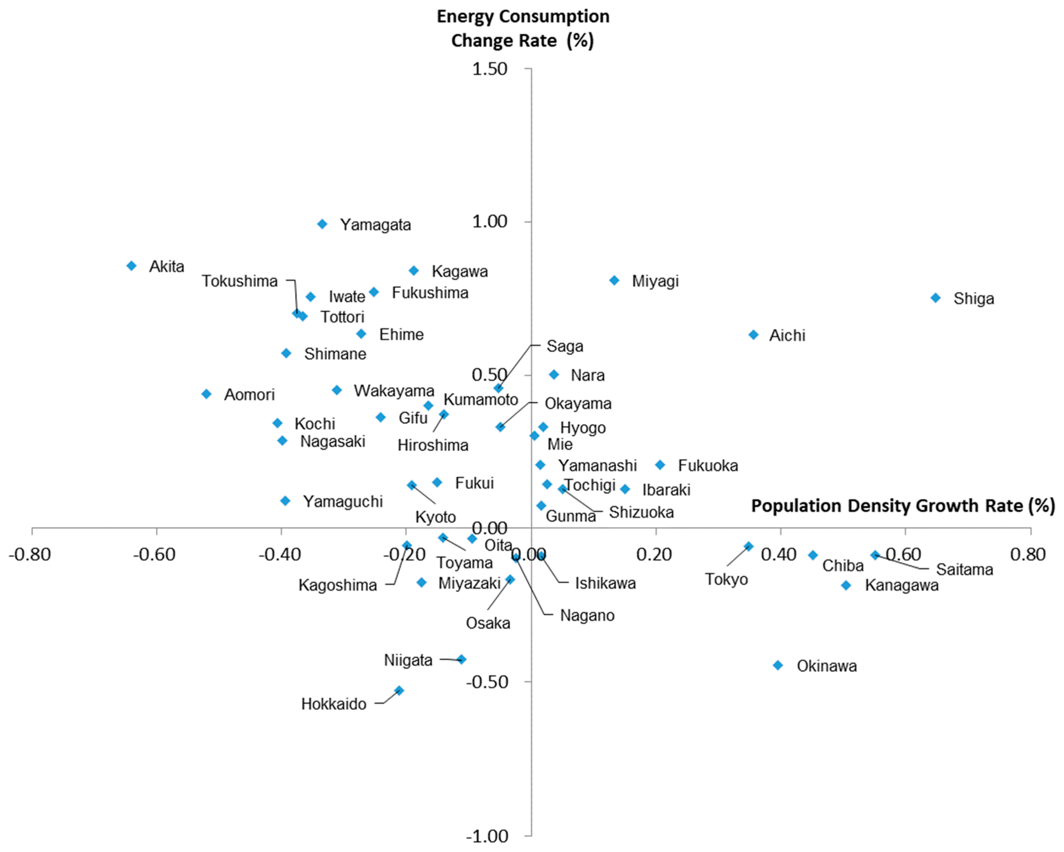Figure 1 plots the relationship between changes in residential energy consumption and changes in population density over the observation period 1990 to 2010. A negative correlation can be highlighted, suggesting the possibility that a rise in population density contributes to reducing energy consumption. For example, the population density of metropolitan areas is rising, but their energy consumption is falling. In Section 3, the extent to which fluctuations in population density affect the changes in energy consumption is stated quantitatively.

To check whether the first-difference GMM estimator of Arellano and Bond [23] suits the data, this study employs panel unit root tests. Specifically, the unit root is assumed to be the individual unit root process (Im et al. [24]), checking for the stationarity of the variables. If the variables are integrated of order 1, I (1), the panel co-integration approach is employed, while if they are I (0), the first-difference GMM estimator (Baltagi [25]) is used. The results of the panel unit root tests are shown in

Table 2. The panel unit root test result.

Test Variables	Without a Deterministic Trend	With a Deterministic Trend
ln EC	−13.93 **	−19.00 **
ln EP	−1.18	6.86
ln IC	−17.33 **	−12.52 **
ln D	−0.11	−2.73 **
ln HS	−5.64 **	−3.15 **
ln FS	2.37	−1.22
ln CDD	−25.36 **	−20.08 **
ln HDD	−27.23 **	−22.01 **

Note: The panel unit root test statistic (Im et al. [24], W-stat) follows a normal distribution, N (0, 1). ** Indicates rejection of the null hypothesis of a unit root at the 1% significance level; and * Indicates rejection of the null hypothesis of a unit root at the 5% significance level.

. The use of the first-difference GMM estimator is justified because the dependent variable (EC) does not have a unit root.

3. Results and Discussion

Table 3. Estimation results.

Regressors	(1)		(2)
Δ ln EC (t − 1)	0.379	**	0.418	**
	(0.012)		(0.012)
Δ ln EP	−0.202	**	−0.191	**
	(0.021)		(0.022)
Δ ln IC	0.344	**	0.319	**
	(0.017)		(0.020)
Δ ln D	−0.412	**	−0.928
	(0.061)		(0.897)
Δ ln D × Δ ln D			0.033
			(0.063)
Δ ln HS	−0.076		−0.024
	(0.080)		(0.089)
Δ ln FS	0.924	**	0.970	**
	(0.124)		(0.141)
Δ ln CDD	0.007	**	0.007	**
	(0.001)		(0.001)
Δ ln HDD	0.036	**	0.062	**
	(0.004)		(0.003)
Number of observations	893		893
J-Statistic	45.677		45.580
Prob (J-statistic)	0.214		0.186
m-Statistic (AR (1))	−5.683	**	−5.393	**
m-Statistic (AR (2))	0.318		0.114
Instruments	EC (t − 2)		EC (t − 2)

Notes: Regressions are estimated using panel data for all prefectures. The two-step first-difference GMM estimation method is used, and standard errors are given in parentheses. The coefficients’ statistical significance is noted at either the 1% level (**) or the 5% level (*). The J-statistic results are obtained from a Sargan–Hansen test for the over-identifying restrictions for the two-step GMM estimators. The m-statistic refers to tests for the first- and second-order serial correlations.

shows the results of Equation (1) dynamic GMM estimations. Model (1) does not consider the nonlinear effects of population density, while Model (2) does.

Dynamic GMM estimation is performed through instrumental variables, consisting of both the available lags of the dependent variable from the second period and the independent variables. The dynamic GMM estimation calls for the Sargan–Hansen test to check for over-identifying restrictions (Hayashi [26]). Under the null hypothesis that all instruments are valid, it can be shown that the test statistics has an asymptotic chi-squared distribution with degrees of freedom equal to the number of over-identifying restrictions. The null hypothesis is not rejected in all models, and thus the estimated models are valid.

The second step of the dynamic GMM estimation requires a test for potential serial correlation of the error terms. In this case, the null hypothesis of no serial correlation for the first-order serial correlation is expected to be rejected, although this does not hold for the null hypothesis on the second-order serial correlation (Baltagi [25]). The test statistics are asymptotically standard normal. The m-statistics in Table 3 test first-order and second-order serial correlations, showing that all the models are appropriate.

Since both the explanatory variables and the explained variables are log-transformed, the estimation parameters can be interpreted as elasticities. Therefore, the greater is the estimated value of the parameter (elasticity), the greater is the effect of the relevant explanatory variable on the explained variable. According to this, the effect of population density tends to be relatively larger than the effects of other variables. Specifically, population density has the second largest effect after residential floor space. In Model (2), the population density terms were not statistically significant, thus not confirming the presence of nonlinear effects of population density. Based on this result, it is possible to move to Model (1).

Within the socioeconomic variables, the energy price (EP) parameter has, as expected, a negative sign. Conversely, the income (IC) parameter is positive, implying an effect on energy consumption. More in detail, a rise in the energy price causes energy consumption to decrease, but a rise in income causes it to worsen. This suggests that a rise in income may cause an increase in energy consumption higher than the rise in income, as the latter leads to purchases of larger household appliances. As for the average household size (HS), no statistically significant effect is found. However, the residential floor space (FS) parameter greatly affects the residential energy consumption.

Table 4. Elasticities.

	Short Run	Long Run
Price	−0.20	−0.33
Income	0.34	0.55
Density	−0.41	−0.66
Average household size	−0.08	−0.12
Floor space	0.92	1.49
Cool	0.01	0.01
Heat	0.04	0.06

shows the short-run and long-run elasticity of the energy saving with respect to each variable calculated from the estimation results in Table 3.

Population density’s elasticity in the short run is −0.41, while, in the long run, it is −0.66. Furthermore, price and income elasticities are small compared to population density elasticity. In other words, the economic factors of price and income do not greatly affect energy consumption compared to the socioeconomic factor of agglomeration.

These results suggest that promoting the formation of urban areas with high population agglomeration might contribute to saving energy consumption. Moreover, as the elasticity of residential floor space is extremely large, thus it can be inferred that this variable is important to ascertain the fluctuations in energy consumption.

Furthermore, this study clarifies the extent to which the determinants of energy consumption have contributed to its variation. Assuming a long-term equilibrium in the partial adjustment model, Equation (1) can be expanded as follows:

$$\Delta E{I}_{jt}=\frac{\alpha }{1-\lambda }\Delta E{P}_t+\frac{\beta }{1-\lambda }\Delta I{C}_{jt}+\frac{\gamma }{1-\lambda }\Delta D_{jt}+\frac{{\delta }^{\prime }}{1-\lambda }\Delta {\mathbf{X}}_{jt}+\frac{\varphi }{1-\lambda }\Delta CD{D}_{jt}+\frac{\eta }{1-\lambda }\Delta HD{D}_{jt}+\Delta {\epsilon }_{jt}$$

(2)

The terms on the right-hand side are, in order, price, income, population aggregation, socioeconomic factor, cooling, heating, and other factors. The observation period covers 20 years from 1990 to 2010. To measure the effect of each individual factor on energy consumption, the estimated coefficients in Equation (1) (from Model (1)) is used to derive Equation (2), from which, in turn, each explanatory variable’s contribution (annual average, %) to changes in energy consumption is calculated.

Looking at the result, the contribution of population density is the largest in the Greater Tokyo area (−0.308%), accounting for approximately half of the decline in energy consumption (

Table 5. Contributions of each factor to changes in energy consumption (1990–2010; annual averages; %).

	Change Rate of Energy Consumption (Δ Energy Consumption = a + b + c + d + e + f + g + h)
	Δ Energy Consumption	Energy Price (a)	Income (b)	Population Density (c)	Average Household Size (d)	Floor Space (e)	Cooling Degree Days (f)	Heating Degree Days (g)	Other (h)
Hokkaido	−0.529	0.103	−0.516	0.140	0.159	0.257	0.054	0.043	−0.769
Tohoku	0.599	0.103	−0.368	0.197	0.144	0.036	0.032	0.049	0.406
Kita-Kanto	0.137	0.103	−0.443	−0.034	0.148	0.344	0.019	0.045	−0.045
Greater Tokyo area	−0.104	0.103	−0.673	−0.308	0.134	0.522	0.017	0.069	0.031
Chubu	0.265	0.103	−0.447	−0.019	0.139	0.308	0.011	0.051	0.120
Hokuriku	0.009	0.103	−0.459	0.061	0.135	−0.097	0.016	0.064	0.187
Kansai	0.335	0.103	−0.601	−0.019	0.142	0.124	0.007	0.050	0.527
Chugoku	0.411	0.103	−0.454	0.178	0.134	0.108	0.006	0.070	0.266
Shikoku	0.630	0.103	−0.342	0.206	0.140	0.133	0.007	0.040	0.343
Kyushu	0.155	0.103	−0.194	0.083	0.139	0.044	−0.002	0.070	−0.088
Okinawa	−0.444	0.103	−0.304	−0.262	0.160	0.029	0.003	0.954	−1.128

Notes: The change rate of energy consumption is the finite difference approximation of the logarithm of the annual average. The regional classification is as follows: Hokkaido (Hokkaido); Tohoku (Aomori, Iwate, Miyagi, Akita, Yamagata, Fukushima, and Niigata); Kita-Kanto (Ibaraki, Tochigi, Gunma, and Yamanashi); Greater Tokyo area (Saitama, Chiba, Tokyo, and Kanagawa); Hokuriku (Toyama, Ishikawa, and Fukui); Chubu (Nagano, Gifu, Shizuoka, Aichi, and Mie); Kansai (Shiga, Kyoto, Osaka, Hyogo, Nara, and Wakayama); Chugoku (Tottori, Shimane, Okayama, Hiroshima, and Yamaguchi); Shikoku (Tokushima, Kagawa, Ehime, and Kochi); Kyushu (Fukuoka, Saga, Nagasaki, Kumamoto, Oita, Miyazaki, and Kagoshima); and Okinawa (Okinawa). Each factor’s contribution is calculated based on the results from the dynamic panel analysis, as shown in Table 3.

). Then, excluding Okinawa, an analogous effect emerges in the large metropolitan areas of Kita Kanto, Chubu, and Kansai. In large metropolitan areas, population agglomeration is advancing, and it seems that urbanization is occurring in parallel with energy efficiency improvements. Conversely, in the majority of the areas other than large metropolitan areas, population agglomeration is not advancing, thus not contributing to saved energy consumption. In particular, energy saving is worsening in Hokkaido, Tohoku, Chugoku, Shikoku, and Kyushu as a result of population dispersion.

Residential floor space is the factor with the largest effect. Due to the increase in the sizes of homes, energy consumption wastage occurs, resulting in its increase. This effect is found in every region, except Hokuriku. On the other hand, it is highly likely that the decrease in income per household leads to the postponement of purchase of energy-using equipment, causing energy consumption to decline. The effects of the declines in income in Hokkaido and Okinawa are significant and lead to saved residential energy consumption.

4. Conclusions

The issue of how to realize economic growth in a context of strengthened environmental restrictions, declining birth rate, and aging population, is important for Japan’s regional economies. This study considered the residential sector to empirically analyze the impact of population agglomeration on energy consumption from a dynamic perspective.

Firms in each region of Japan are promoting improvements to energy efficiency through the development of energy-saving technologies, while facing global competition. However, in the residential sector, insufficient progress has been made in improving energy efficiency. In previous research conducted in Europe and the US, it has been shown that households in regions characterized by population agglomeration consume less energy. Even in the empirical analysis of this study, the possibility of decreasing energy consumption in areas where population agglomerates has been highlighted. The existing analyses have primarily been cross-sectional, and they have not sufficiently clarified the main result from a dynamic perspective. On the contrary, in this study, through a partial adjustment model, we are able to capture the mid- to long-term impacts of population agglomeration on energy consumption.

Specifically, the results confirm that population agglomeration causes energy consumption to decrease in the residential sector. In other words, agglomeration economies that occur alongside population agglomeration bring about high energy efficiency. However, regional differences are present. On the one hand, the contributions of population agglomeration are seen in the major metropolitan areas of the Greater Tokyo area, Chubu, and Kansai; on the other hand, in rural areas, excluding Okinawa, population dispersion is progressing, causing energy savings to worsen. Therefore, to improve energy efficiency in Japan, it will be necessary to raise population aggregation not only in major metropolitan areas but also in rural areas. The compact city policy to populate the city center may be effective in this respect.

Many large cities are located in the regions of Greater Tokyo area, Chubu, and Kansai, and these regions enjoy the benefits of agglomeration economies thanks to the agglomeration of various industries that differ in structure (Otsuka [27]). Increasing the diversity of industrial structures would imply increasing both productivity and energy efficiency. Conversely, in rural regions, large cities are missing, with small-sized cities prevailing. The latter can enjoy the benefits of localization economies, that is, economies based on the agglomeration of firms within the same industry. To enjoy these benefits without suffering the uneconomical aspects of large-city agglomeration (e.g., overcrowding and soaring land prices), a city should ideally be kept small by specializing in selected industries (Henderson [28]). The relationship between city sizes and energy consumption should be the agenda of future research. To identify the desirable city size to realize a low-carbon society, it is necessary to quantitatively grasp the optimal population size allowing the increase in energy efficiency.