Article

Sustainable Inventory Management for Environmental Impact through Partial Backordering and Multi-Trade-Credit-Period

1
Department of Industrial & Management Engineering, Hanyang University, Ansan, Gyeonggi-do 155 88, Korea
2
Department of International Business, Cheju Halla University, Jeju-do 63092, Korea
*
Author to whom correspondence should be addressed.
Sustainability 2018, 10(12), 4761; https://doi.org/10.3390/su10124761
Submission received: 4 November 2018 / Revised: 5 December 2018 / Accepted: 9 December 2018 / Published: 13 December 2018

Abstract

:
Incorporation of sustainable management for the rework of defective items brings long lasting benefits. In global business, there are situations when the products are procured from a global supplier. There are chances that the received lot may contain a fraction of imperfect products. These imperfect products are still valuable and can be repairable to save the environment. It is sustainable to repair imperfect items in a local repair store as compared to sending it back to the supplier. The cost of carbon emissions is also incorporated in the function to incorporate the environmental impact on total profit. Meanwhile, the supplier also offers a multi-trade-credit-period to the buyer. The developed model is sustainable and reduces the environmental impact as well as benefits for interim financing. This paper has an objective to maximize the total profit by developing a synergic economic order quantity model by considering multi-trade-credit policy, rework, and shortages simultaneously. This model can help in making decisions to enhance the performance of sustainable inventory management by controlling the cycle time and a fraction of time for a global supply chain. A non-derivative approach is employed to develop a closed-form optimal result. The numerical illustration with sensitivity analysis is also drawn to provide managerial insights into real practices.

1. Introduction

In global business for a sustainable environment, production managers implement and apply efficient production planning under control systems to get 100% perfect items at an economized cost. However, the production system may still manufacture imperfect items. The imperfect items cut down the income of the buyer and also have a negative impact on the environment by focusing on the extra activity required to exchange these imperfect items with the global supplier. This unintentional supply to the customer may cause a loss of goodwill. Nowadays, in order to buy sustainable products or sustainable raw material at an economical cost in the global supply chain, the buyer first finds out the suppliers in global bourses and then work out the best one. As buyers and suppliers are located far away, this also makes it impossible for a supplier to send the buyer all perfect items. Thus, to ensure good quality and brand reputation, it is mandatory for the buyer to inspect an entire lot as soon as it comes into an inventory. After the screening of items, it may be possible that some percentage of items is identified as defective items with minor damage. These imperfect product items are valuable products. The exchange of imperfect items with an urgent shipment is not suitable and also it puts a negative impact on the environment because the manufacturer is located miles away from the buyer. If the exchange of defective products is going to happen with a global supplier, then it will increase the environmental cost, which in turn also increases the total cost of the system. These minor damages can be repaired at a local repair shop. In order to maintain the sustainable supply of products at an economical cost and to reduce the environmental impact, reparation of these items at a local repair shop as compared to exchanging them with the supplier is a sustainable approach.
To be competitive, firms can no longer work as an independent and single entity but as a mutual part of the business. As a result, firms are grasping the importance of better understanding of, and cooperation with, their suppliers and buyers. Efficient inventory management and the financial system plays a significant role in the profit of the business. In modern business models, trade credit time is a challenge for businesses. Currently, trade credit becomes a win-win strategy for buyers and suppliers. It adds an extra interest or an opportunity cost for the supplier and buyer, therefore delayed time is an important subject that researchers should consider while developing inventory models. In inventory model assumptions, the buyer instantly pays the cost of the product to the supplier as the products are shipped to the buyer. Conversely, in real corporate business transactions, the supplier often allows a delayed period for the buyer to settle down the payments. This fixed and allowable period for relaxing the payments allows the supplier to minimize on-hand stock and improve sales. Also, during this allowable time, the buyer keeps selling items without paying back to the supplier and enjoys the additional amount of interest income from these sales. Trade credit financing is considered to be a dominant application to enhance sales and maximize profits for businesses. Due to this, the opportunity cost and interest income is incorporated into the model to calculate the total profit.
The domain of inventory management has acquired a lot of importance from experts as well as researchers in the industry. It is worth mentioning to indicate that one of the impractical assumptions in the inventory framework that has established significant consideration by academics and researchers is that all products in a received lot have the desired quality. The assumption of instant payment is also relaxed in the proposed model. Due to these unrealistic facts, an inventory model with imperfect quality and the sustainable reparation of imperfect items to reduce environmental concerns under partial backordering and delay in payments is considered. In order to get an effective solution of the algorithm, an algebraic approach is utilized for profit maximization. This methodology is a non-derivative approach to avoid using derivative information in the classical sense to find optimal solutions. It develops a closed-form optimal solution and gives effective results for our objective. This methodology is efficient and the simplest way for explaining the inventory theory and reducing the likelihood of errors. This study also contributes an insight for industrial managers for the supply of electric circuits such as home appliances and automobile assemblers. In many cases, the needed products are purchased in advance by these companies from some far away supplier. Thus, if some percentage of these procured products are identified as imperfect quality, the exchange of these are not possible instantly due to large distances between them. Instead of increasing the shipment cost and to put a negative impact on the environment, these imperfect items are repaired in the local repair shop, which is more sustainable as compared to sending it back to the supplier. Furthermore, in such circumstances, these firms are allowed to incur shortages which are backordered.
The overview of this research paper is as follows: A literature review is written in Section 2. The problem definition, notation, and assumptions developed in the proposed inventory model are stated in Section 3. Formulation of a mathematical model for each case is presented in Section 4. The numerical example with results in detail is expressed in Section 5. Section 6 discusses the sensitivity analysis due to a change in key parameters. Managerial insights are written in Section 7. Finally, the conclusions of this study and potential future extensions are given in Section 8.

2. Literature Review

In recent years, the subject of imperfect products has gained the attention of academicians and researchers. It is noteworthy to state that it is an unrealistic assumption that all products during manufacturing or in the received lot is according to the desired quality. This assumption is impractical to satisfy and it is a restriction in the established EOQ inventory model. Porteus [1] studied the correlation among the percentage of imperfect products and the lot when the assembly line is not under control. Rosenblatt and Lee [2] discussed that lot size should be of a smaller size in order to avoid defective items. This is due to the assumption that the fraction of defects depends upon the lot size. Salameh and Jaber [3] extended the EOQ model for imperfect items by considering the random fraction of imperfect products in a lot. According to them, shortages are disallowed and poor-quality items are investigated using a screening procedure. They also state in their study that defective items are still valuable products and can be used. Eroglu and Ozdemir [4] further extended the study and proposed the EOQ model in which they examined that each lot that is inspected must contain defective items, and due to this, shortages are backordered. Roy et al. [5] developed an EOQ model with a fraction of the lot not being products of the desired quality. The stock-out condition occurs during a screening of the total lot. Due to stock-out, a partial percentage of the demand is fulfilled via partial backordering and the remaining demand is taken as lost sales. Vörös [6] proposed an economic order and production quantity models without constraint on the fraction of imperfect items. Afterward, Hsu and Hsu [7] investigated the EOQ model and proposed that due to inspection failure, there will be the occurrence of type I and type II errors. Also, these defective quality and screening errors create a shortage. Rad et al. [8] developed a combined supplier–buyer supply chain model with a demand rate dependent on price. An imperfect item and backorder are considered in the proposed model.
The relation of environmental impact due to imperfect items also entails a serious risk for a sustainable supply process. Kazemi et al. [9] investigated the effect of carbon emissions in an imperfect supply process. They studied the inventory model with imperfect quality under the sustainable point of view. Marchi et al. [10] proposed a vendor–buyer green supply chain model by considering both a decentralized and a centralized optimized policy. They consider investing in learning in production and in reducing carbon emissions of the production process. Bazan et al. [11] established that optimizing the environmental cost and total cost jointly promotes less remanufacturing to save the environment. Wahab et al. [12] proposed a sustainable inventory model for a global supply chain by taking into consideration imperfect items and environmental impact. Taleizadeh et al. [13] developed a sustainable economic production quantity model under shortages for the inventory system. The proposed model can be selected by managers based on the dependence of manufacturer’s motivations to increase the service level. Taleizadeh et al. [14] introduced a two-layer green supply chain with a rework of imperfect units under a bi-level credit period. The upstream and downstream credit period in the system helps to stimulate demand as well as sales and reduce inventory. Sarkar et al. [15] calculated the joint effects of variable emission cost and multi-delay-in-payments for a global sustainable supply chain. Kim and Sarkar [16] proposed a multi-stage cleaner production system by eliminating all defective items during the production process. Moshtagh and Taleizadeh [17] explained a closed loop supply chain model of stochastic integrated remanufacturing and manufacturing model with rework, shortage, and quality-based return rates. Li et al. [18] provided primary evidence concerning the impact of commercial quality management on green invention and the moderating role of environmental regulation on this relationship. Ahmed and Sarkar [19] describes the impact of carbon emissions in a sustainable supply chain management for second-generation biofuel. Younesi and Roghanian [20] designed a framework for sustainable product design based on quality function deployment for the environment. They considered cost, quality, and environmental factors for sustainable product design, which helps designers to make healthier decisions.
Skouri et al. [21] considered a single echelon inventory system under the traditional EOQ paradigm with backorders to analyze the effects of lot quality on cost performance. They state that previous studies on imperfect quality are focused on variations of the proportional yield, where the supply lot after screening the defects are accepted and then used. In their model, they study a substitute setting where the whole shipped lot may be below the quality criteria and, as a result, rejected on arrival. Chakraborty and Giri [22] studied the lot sizing in a production system under imperfect maintenance, inspection, and reworks. They consider a deteriorating production system in this model. Sarkar et al. [23] developed an economic production model with a reworking process for defective items with planned backorders. Jaber et al. [24] proposed an EOQ model for imperfect quality, reworking, and emergency purchases from a local store at a higher cost. Sharifi et al. [25] analyzed the impact of screening errors in an EOQ model with partial backordering and calculated the optimal order size and number of backordering units. In the same year, Taleizadeh et al. [26] considered an imperfect production model with a two-level trade credit period and backordered demand. Also in the same year, Zhou et al. [27] introduced a synergic EOQ inventory model with a trade credit period, imperfect quality, screening errors, and full backordering. Taleizadeh et al. [28] presented an EOQ inventory model in which according to time, the rework items are entered into the initial inventory system. Sarkar and Saren [29] proposed a production model with consideration of the item inspection policy, inspection errors, and warranty cost for non-screened products. In their study for the case of 100% inspection, the expected total cost with screening cost leads to a higher cost of inventory. Dey [30] examined an integrated single-buyer, single-vendor inventory model with defective production under a diverse environment where randomness and fuzziness appear simultaneously. Kang et al. [31] proposed an inventory model on the basis of work-in-process by integrating the impact of the random imperfect rate on lot size.
The efficacy of business is increased via cooperation and mutual understanding between firms. The performance of the supply chain can be improved by facilitating longer payment terms for buyers and better access to financing for suppliers [32]. The financial flows between organizations of the supply chain, however, were often neglected and have only recently found greater attention in the academic literature [33]. Trade credit is the financial approach that is offered by the supplier to the buyer. During this course of action, the buyer is endorsed with a time period to return back the payment for purchased units without any interest. In this period, the buyer also does not pay any interest on items stored in the warehouse. In contrast, the penalty is charged if the payable amount for the purchased items is not returned within this allowable time. The supplier has the advantage to interest the buyer in buying the products in enormous batches. On the other hand, the existence of trade credit will benefit a supplier’s sales and lessen the stock level. In the meantime, the buyer can get the interest income on these sales. Goyal [34] was the first to introduce the inventory model with the permissible delay-in-payments under constant demand. Chand and Ward [35] further extended Goyal’s [34] model by taking the assumptions of a traditional optimum order quantity paradigm and obtained different results. Shah [36] proposed an inventory model with probabilistic time scheduling for an exponentially decaying inventory when the supplier offers trade credit for matching the accounts for the procure order quantity. Huang [37] drew out an EOQ model under multi-level-delay-in-payments. Soni and Shah [38] proposed an EOQ mathematical model to frame the optimal ordering policy for the buyer, where demand is taken to be partially dependent on stock level and partially constant, and the supplier also gives progressive credit periods. Tsao et al. [39] explained the impact of a maintenance policy on imperfect production process with a trade credit policy. Sana et al. [40] presented a three-level supply chain model for multi-products. Yang and Tseng [41] proposed a model of the multi-echelon supply chain with trade credit by considering the backorder and a controllable lead time. Jaggi et al. [42] studied an inventory model with allowable shortages and trade credit for different circumstances. Soni et al. [43] designed an integrated supplier–buyer inventory framework that has variable production and defective items with a partial trade credit policy. Tsao and Linh [44] introduced a network design of supply chain partial backordering and trade credit policy. The previous studies show that the trade credit policy between the supplier and buyer is joint bartering. It is acclaimed that the trade credit approach that is given by most researchers offers a single permissible delay-in-payment. In a wide range of global business, a trade credit policy for inventory systems has been given a lot of attention by many researchers. Giri and Sharma [45] investigated an inventory model having a linear time-dependent demand with allowable shortages and two levels of trade credit. Tiwari et al. [46] developed a sustainable production quantity model with random imperfect quality items, trade-credit policy, service level constraints, and failure in reworking. Tsao et al. [47] considered an inventory model with ordering for non-instantaneous deteriorating products and two-tiered pricing under a trade credit policy. Banu and Mondal [48] analyzed an inventory system having an effect of customers’ credit on the given demand function with two-level credit financing. A fuzzy environment was considered in this model by assuming uncertainties in the credit period.
From the above-mentioned literature, for continuing the applied practice, this study considers a sustainable inventory management of reworking products on environment by considering the multi-delay-in-payments in a single level, and partial backordering in the inventory model. The arrival of rework items is taken into account when the initial inventory system reaches the zero level. Also, in today’s business environment, trade credit is the desirable foundation of interim financing for firms. The contribution and input of authors are presented in Table 1.

3. Problem Definition, Notation, and Assumptions

The section presents the problem definition, notation consisting of decision variables and parameters, and assumptions of the proposed model.

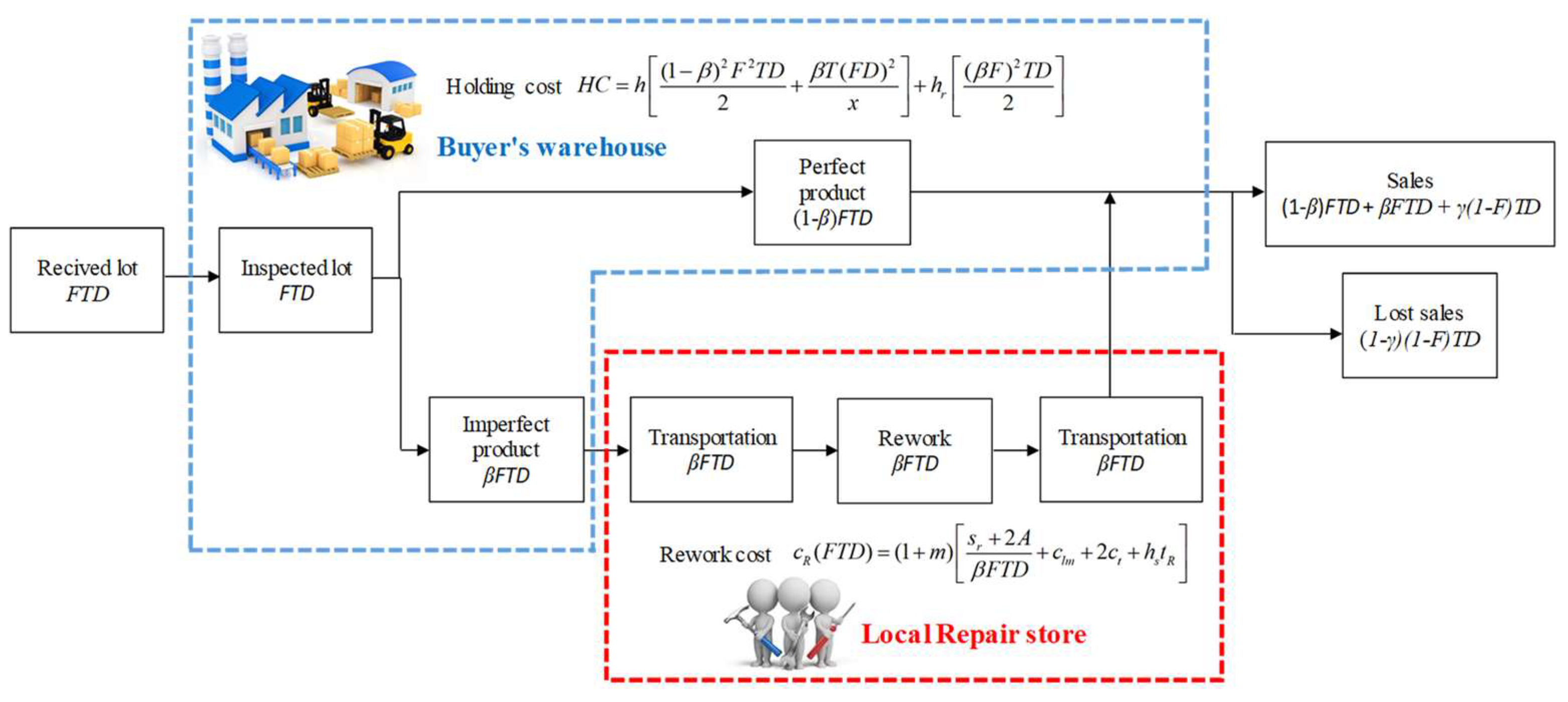
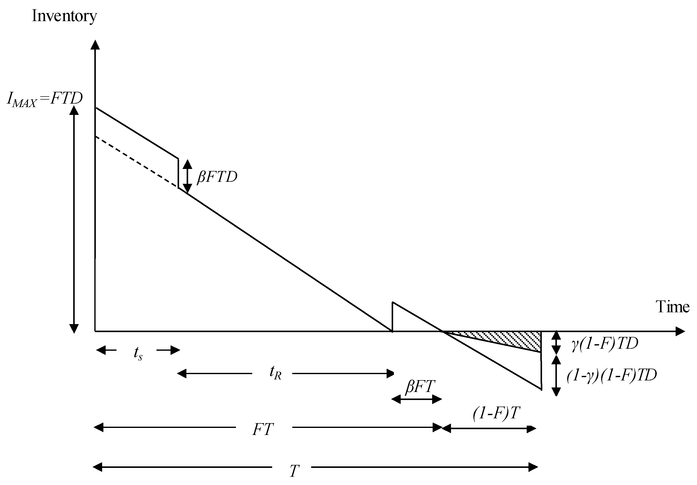
3.1. Problem Definition

A situation is developed in which buyer purchases the products from a supplier that is situated miles away. There is a possibility that either in process failure due to imperfect production system or as a result of the mismanaging of products in the course of transportation, the received lot may contain a few imperfect products. After screening the products, it is identified that some percentage of products do not meet the desired quality. These imperfect products must be exchanged by desired quality products in order to fulfill the required demand. It is assumed that these imperfect products can be reworked at a local repair store. As the supplier is located far away, the shipment cost and environmental impact for these exchanged products are very high compared to the repair cost. It is decided that these imperfect products are to be repaired at a local repair store in order achieve sustainability. Therefore, at the end of the screening process, these imperfect products are transported to a repair store immediately. After the reparation of products, they are entered in the initial inventory and the holding cost of initial inventory is less than the holding cost of repaired products. The repair store consists of variable and fixed costs. The fixed cost consists of the setup cost of the repair store and the fixed transportation cost of imperfect products. The variable cost contains unit shipment cost per imperfect product, material and labor cost per imperfect product, and holding cost per reworked product at a repair store. According to the time, it is assumed that repaired products came back to the buyer when the initial inventory level becomes zero. It is also supposed that the buyer is giving payment to its supplier under the multi-trade-credit-period policy. Under the given conditions of multi-delay-in-payments, the supplier permits the buyer a multi-payment period. Interest is earned or charged during these multiple permissible periods. The allowable durations to return the payment will affect the interest charged and interest earned. If the buyer sells the products before the permissible payment period, then the interest is earned by sales returns. However, if they fail to make the payment in this given time, then an interest is charged to the buyer according to given interest rates. Thus, the main objective is to design a sustainable inventory management that can reduce the environmental impact by optimizing the lot size (Q), which can be done via optimizing the cycle time (T) and a fraction of cycle time (F) under partial backordering due to reworking of the imperfect items and multi-trade-credit-period. Figure 1 shows the inventory system of the imperfect quality product and rework.

3.2. Notation

Decision variables
T 
cycle time (time unit)
F 
fraction of time that has a positive inventory level (%)
Dependent variable
Q 
Order size per cycle (units)
Parameters
D 
demand rate per unit time (units/time unit)
X 
screening rate (units/time unit)
ts 
screening time of products (time unit)
tR 
transportation, rework, and return time for imperfect products (time unit)
tT 
total transportation time of imperfect products (time unit)
R 
rework rate (units/time unit)
A 
fixed cost of transportation ($/trip)
β 
percentage of imperfect items (%)
O 
ordering cost of buyer ($/order)
sr 
setup cost of repair store ($/setup)
h 
holding cost of perfect items ($/unit/time unit)
h’ 
carbon emission cost per item on holding perfect items ($/unit/time unit)
hr 
holding cost of rework products ($/unit/time unit)
hr 
carbon emission cost per item on holding rework item ($/unit/time unit)
hs 
holding cost at repair store ($/unit/time unit)
hs 
carbon emission cost per item on holding item at repair store ($/unit/time unit)
Cs 
screening cost per unit ($/unit)
Cu 
purchasing cost of one unit ($/unit)
ct 
transportation cost of the imperfect item per unit ($/unit)
clm 
labor and material cost required to repair a unit product ($/unit)
l 
cost incurred due to a loss of sales ($/unit/time unit)
g 
penalty cost incurred due to goodwill loss (S/unit)
w 
percentage of imperfect items passed to customers (%)
u 
unit return cost of the imperfect product (S/unit)
π 
backordered cost ($/unit/time unit)
P 
selling price of one unit (S/unit)
γ 
percentage of backordered demand (%)
m 
markup percentage by rework store (%)
M 
first permissible delay period for payment (time unit)
N 
second permissible delay period for payment (time unit)
Ie 
interest earned (%)
Ic1 
interest charged for period M (%)
Ic2 
interest charged for period N (%)

3.3. Assumptions

The mathematical model is structured on the following assumptions.
  • The inventory system has a single type of product.
  • Warehouse carbon emission is due to the energy consumption per unit item. Thus, according to carbon tax policy, carbon emission cost per unit item h’, hr, and hs is considered for holding perfect items, holding repair items, and holding items at the repair store, respectively.
  • There is a chance to receive a lot with a fraction of defective items from a global supplier, which is from other country.
  • Shortages are allowed and these are partially backordered.
  • Demand and inspection rates are considered as constant and known.
  • The screening process and demand occur at the same time, but the screening rate is faster than the demand rate (x > D).
  • Imperfect products have minor damage and can be repairable in a controlled system and all imperfect products are reworked.
  • The percentage of imperfect products are given and known.
  • The relationship between the purchasing cost of buyer Cu and selling price of buyer P is PCu.
  • The holding cost of reworked products is higher than the initial holding cost of perfect items (hR > h).
  • The reworked products are returned back when the inventory level of the system becomes zero.
  • As the shipment lot is received, the backordered demand is fulfilled first.
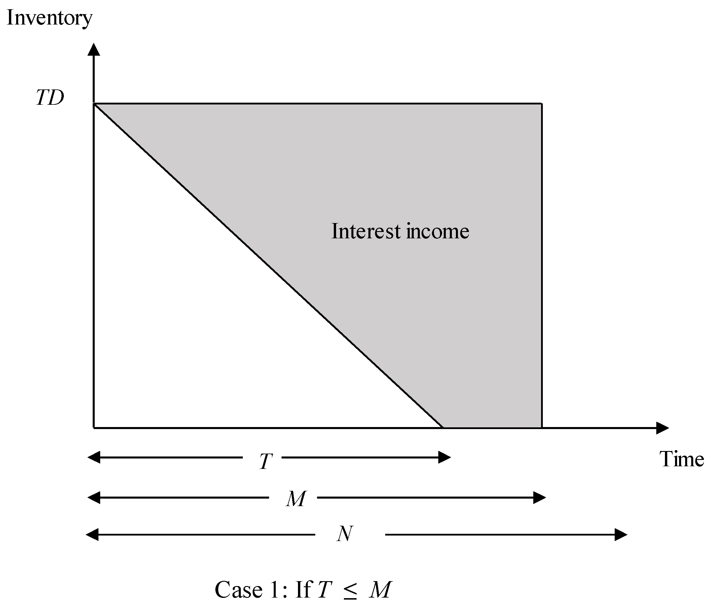
  • The supplier allows a multi-trade-credit-periods M and N to the buyer. During these periods, the buyer sells the product and utilizes its income to earn interest with rate of Ie.
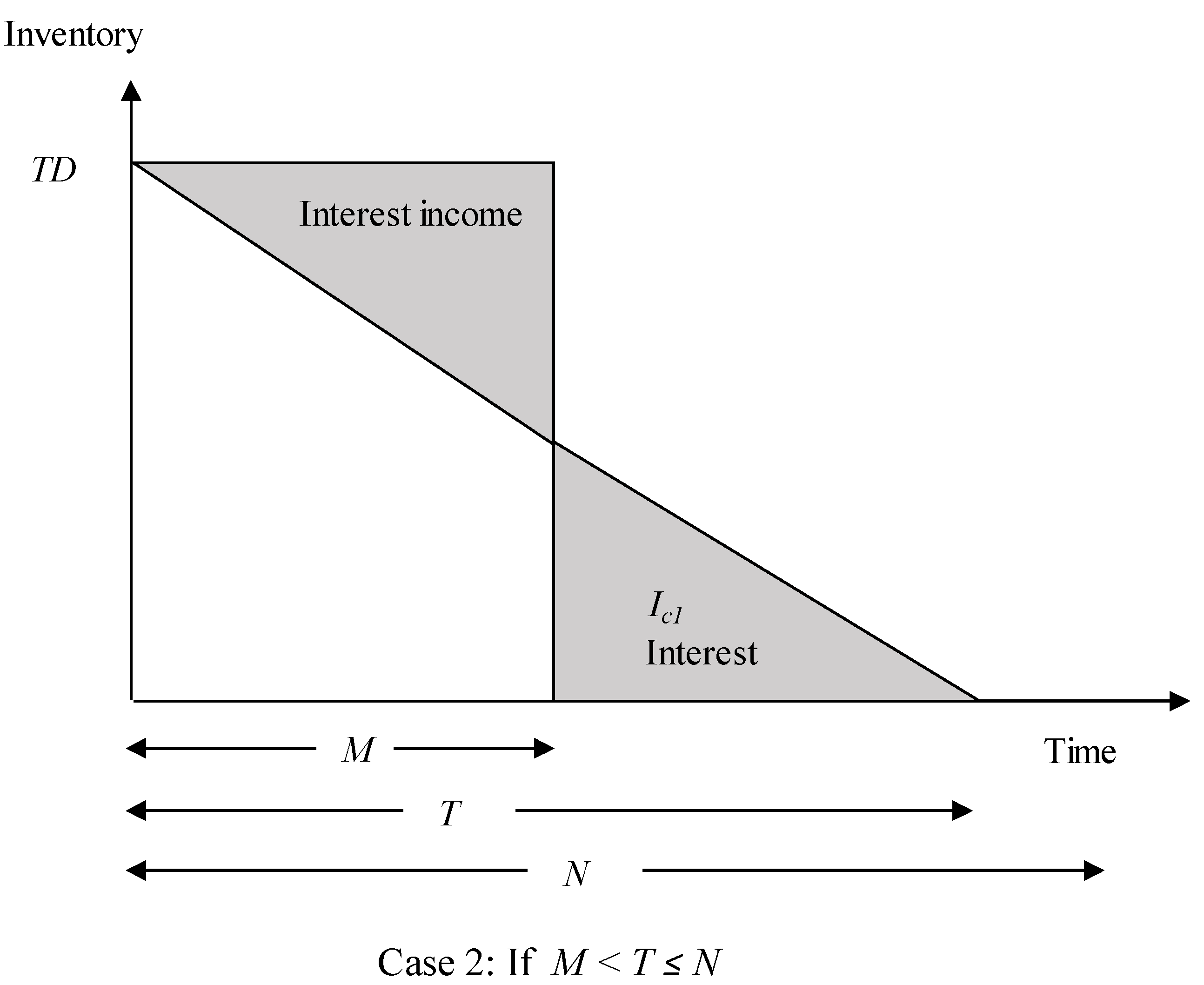
  • If the buyer fails to make the payment to the supplier during the first credit period M, then interest Ic1 is charged, and later if the buyer again fails to make the payment to the supplier during second allowable time N, then additional interest is also charged at a rate of Ic2.
  • The percentage of defective items are sent to customers, which are returned back to the buyer in the next cycle. The buyer pays a cost per unit for these returned products and a cost per unit as a penalty cost incurred due to goodwill loss.

4. Mathematical Modeling

This section describes and develops an integrated sustainable inventory model of total profit with a multi-delay-in-payments, partial backordering, and reparation of imperfect products. To investigate imperfect items, the entire lot is screened at a rate x during the inspection time t s = I M A X / x . The demand rate is less than the inspection rate (D < x). After the inspection period ts, the items that do not meet the desired quality characteristics are taken out of inventory and sent to the repair store. The repaired items come back to the system after tR amount of time. The tR is the cumulative time of transportation and repair times. The repairing process at the local repair store works in a controlled system. The sr + 2A is the fixed cost of the repair shop, where s is the setup cost of the repair shop and A is taken as the fixed cost of transportation. The variable cost is given by c l m + 2 c t + ( h s + h s ) t R per imperfect product at repair store, where c l m is labor and material cost, c t is transportation cost, hs is the holding cost at repair store, hs is the carbon emission cost per item on holding an item at the repair store, and tR is the total repair duration, which consists of the transportation time, return time, and repair time of imperfect items. The repair duration is given by t R = t s + β F T D / R . The total cost for repair shop is taken to be s r + 2 A + β F T D   ( c l m + 2 c t + ( h s + h s ) t R . The holding cost of the repaired product is given by hr. If h is the initial unit holding cost, then h < hr. The positive inventory level of the system is taken to be FT, and (1 − F)T is the duration of the time in which the shortage takes place. It is assumed that the repaired products come back in the system when the level of inventory is zero. During the start of the cycle, FTD is the level of inventory. The products are inspected at rate x and the screening time is given as t s = F T D / x . After inspection, it has been found that a fraction β of products is imperfect. These imperfect items are taken out of the system and sent to the repair shop. If the shortage quantity is given by (1 − F)TD, then γ(1 − F)TD is the backordered amount shortage, and (1 − γ)(1 − F)TD is the loss of sales quantity. Figure 2 illustrates the detailed inventory behavior of the desired system.
Ordering Cost
At the start of each cycle length T, the buyer incurs a one-time ordering cost (OC) per unit time, where O is fixed ordered cost and it is given as:
O C = O T
Inspection Cost
The total inspection cost of the whole lot is denoted by IC, and is given as:
I C = C s F D
where Cs the inspection cost of one unit, F is the duration of positive inventory time, and D is demand rate.
Holding Cost
The total holding cost per time unit is a combination of the holding cost of perfect products that are already in the system and the holding cost of repaired products, and is given as:
H C = ( h + h ) [ ( 1 β ) 2 F 2 T D 2 + β T ( F D ) 2 x ] + ( h r + h r ) [ ( β F ) 2 T D 2 ]
Rework Cost
If a margin m is claimed as the repair charge per unit, then the repair cost (cR) for one unit is expressed as:
c R ( F T D ) = ( 1 + m ) [ s r + 2 A β F T D + c l m + 2 c t + ( h s + h s ) t R ]
The repaired products come back into the inventory when the initial inventory level becomes zero, therefore the level of inventory becomes β F T D units. As the cycle ends, (1 − F)TD becomes the shortage level of the system. The order quantity for a given cycle is considered to be Q = F T D + γ ( 1 F ) T D .
Shortage Cost
If π is the backordered cost, l is the cost of loss of sales and γ is a percentage of backordered demand, then the shortage cost per unit time is expressed as:
S C = γ ( 1 F ) 2 T D 2 + l ( 1 γ ) ( 1 F ) D
Goodwill Penalty Cost
If v is the unit return cost of a product and g is unit penalty cost from goodwill loss, and there is w percentage of imperfect items that are passed to the customers, then the goodwill penalty cost is given as:
G W C = ( v + g ) w F D
Interest Charged and Interest Income Earned
According to the trade credit policy, if the allowable payment duration is larger than the lead time, it brings interest income to the buyer. If this allowed time is smaller than lead time, then it would bring more opportunity cost and less interest income to the buyer; meanwhile, the supplier can earn interest income and pay less opportunity cost. Due to this fact, the supplier’s model has the two following cases, based on the permissible time of payment X and length of lead time, the different cost between two likely cases are as follows.
Condition 1.
If the lead time T is smaller than or equal to the permissible payment period M given to the buyer by the supplier, then only interest income is earned as interest charged in such a condition is zero. It is drawn in Figure 3, and is given as:
Interest   income   =   P I e [ D M T D 2 ]
Condition 2.
If the lead time T is larger than the first allowable payment time M and smaller than or equal to second allowable payment time N given to the buyer by the supplier, then both interest cost are charged and earned. Figure 4 illustrates the given condition and it is given by the following expression:
Interest   income   =   P I e ( D M ) 2 2 T D
Interest   charged   =   C u I c 1 ( T D D M ) 2 2 T D
Condition 3.
There is a special case in which extra interest is charged to the buyer if they fail to give the required payment in the first allowed time. In this case, the lead time T is larger than the second allowable payment time N given to the buyer by the supplier. The presentation of this given condition is shown in Figure 5. The interest charged and interest income is given as:
Interest   income   =   P I e ( D M ) 2 2 T D
Interest   charged   =   C u I c 2 ( T D D N ) 2 2 T D C u I c 1 D T ( N T N 2 M T + M N ) C u I c 1 D ( N M ) 2 2 T
Total profit function
Total profit = Selling price − [Ordering cost + Product cost + Inspection cost + Holding cost + Rework cost + Shortage cost + Goodwill penalty cost +Interest earned –Interest charged]
According to these different conditions of multi-delay-in-payments, three cases are developed and the total profit function for all cases can be given as:
Case 1. 
Total Profit (TP1) if T ≤ M:
T P ( F , T ) = P D ( F + γ ( 1 F ) [ O T + C u ( F D + γ ( 1 F ) D ) + C s F D + ( h + h ) [ ( 1 β ) 2 F 2 T D 2 + β T ( F D ) 2 x ] + ( h r + h r ) [ ( β F ) 2 T D 2 ] + π ( 1 F ) 2 γ T D 2 + β F D ( 1 + m ) [ s r + 2 A β F T D + c l m + 2 c t + ( h s + h s ) ( β F T D R + t T ) ] + l ( 1 γ ) ( 1 F ) D + ( u + g ) w F D + P I e [ D M T D 2 ] ]
Case 2. 
Total Profit (TP2) if M < T ≤ N:
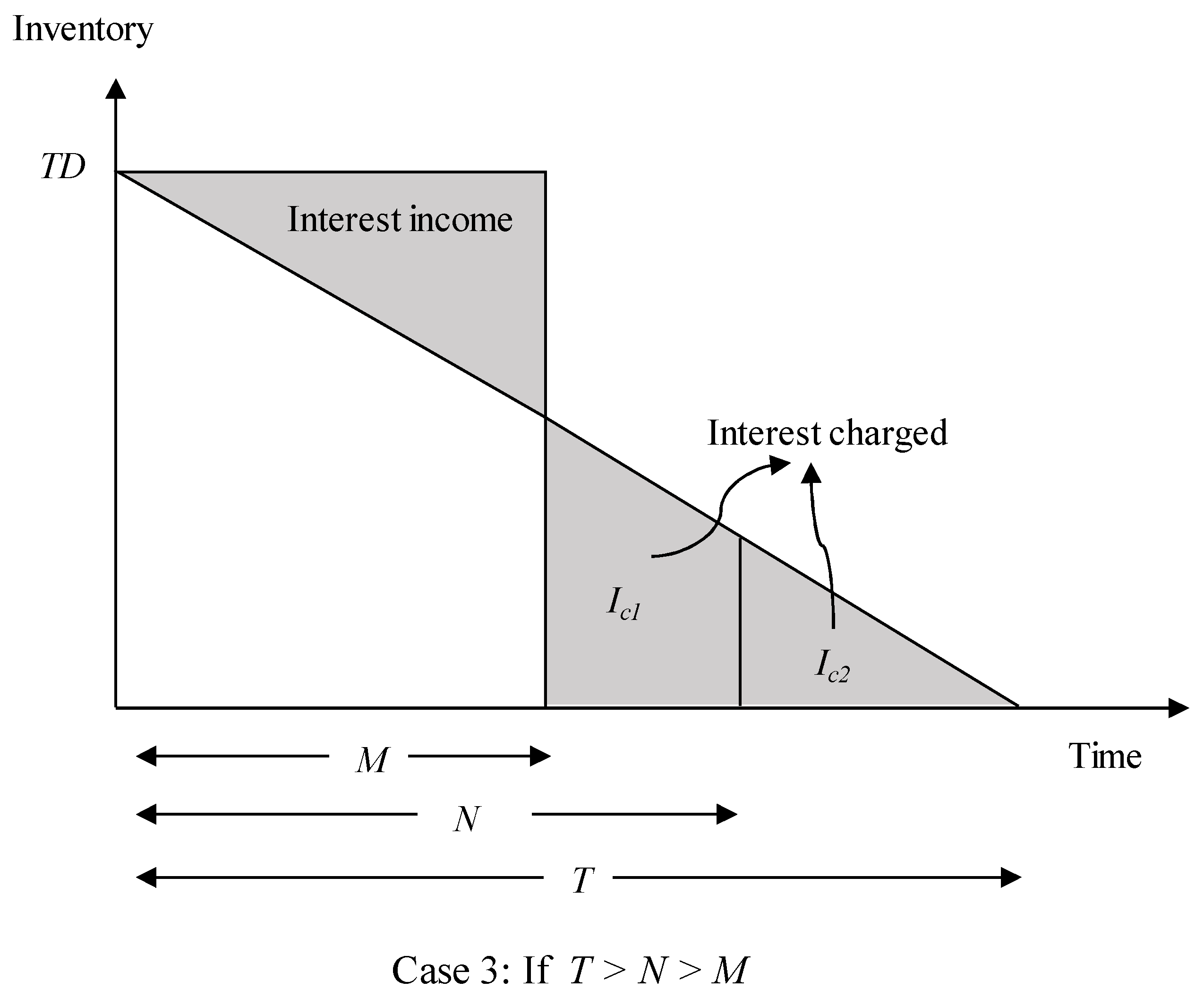
T P ( F , T ) = P D ( F + γ ( 1 F ) [ O T + C u ( F D + γ ( 1 F ) D ) + C s F D + ( h + h ) [ ( 1 β ) 2 F 2 T D 2 + β T ( F D ) 2 x ] + ( h r + h r ) [ ( β F ) 2 T D 2 ] + π ( 1 F ) 2 γ T D 2 + β F D ( 1 + m ) [ s r + 2 A β F T D + c l m + 2 c t + ( h s + h s ) ( β F T D R + t T ) ] + l ( 1 γ ) ( 1 F ) D + ( u + g ) w F D + P I e ( D M ) 2 2 T D C u I c 1 ( T D D M ) 2 2 T D ]
Case 3. 
Total Profit (TP3) if T > N:
T P ( F , T ) = P D ( F + γ ( 1 F ) [ O T + C u ( F D + γ ( 1 F ) D ) + C s F D + ( h + h ) [ ( 1 β ) 2 F 2 T D 2 + β T ( F D ) 2 x ] + ( h r + h r ) [ ( β F ) 2 T D 2 ] + π ( 1 F ) 2 γ T D 2 + β F D ( 1 + m ) [ s r + 2 A β F T D + c l m + 2 c t + ( h s + h s ) ( β F T D R + t T ) ] + l ( 1 γ ) ( 1 F ) D + ( u + g ) w F D + P I e ( D M ) 2 2 T D C u I c 2 ( T D D N ) 2 2 T D C u I c 1 D T ( N T N 2 M T + M N ) C u I c 1 D ( N M ) 2 2 T ]
where P is the selling price per unit, Cu is the product cost per unit, Ie is interest earned per unit, Ic1 is interest charged per unit for the permissible delay period M, and Ic2 is interest charged per unit for permissible delay period N.

4.1. Optimal Values of F and T for Case 1

The profit function for Case 1 in Equation (12), found by adding +1 and −1 to the order quantity, is given as:
T P ( F , T ) = P D ( 1 ( 1 F ) ( 1 γ ) [ O T + C u D ( 1 ( 1 F ) ( 1 γ ) ) + C s F D + ( h + h ) [ ( 1 β ) 2 F 2 T D 2 + β T ( F D ) 2 x ] + ( h r + h r ) [ ( β F ) 2 T D 2 ] + π ( 1 F ) 2 γ T D 2 + β F D ( 1 + m ) [ s r + 2 A β F T D + c l m + 2 c t + ( h s + h s ) ( β F T D R + t T ) ] + l ( 1 γ ) ( 1 F ) D + ( u + g ) w F D + P I e [ D M T D 2 ] ]
Rearranging the terms, this can be expressed as:
T P ( F , T ) = P D C u D [ O T + C s F D + ( h + h ) [ ( 1 β ) 2 F 2 T D 2 + β T ( F D ) 2 x ] + ( h r + h r ) [ ( β F ) 2 T D 2 ] + π ( 1 F ) 2 γ T D 2 + β F D ( 1 + m ) [ s r + 2 A β F T D + c l m + 2 c t + ( h s + h s ) ( β F T D R + t T ) ] + l ( 1 γ ) ( 1 F ) D + ( u + g ) w F D + P I e [ D M T D 2 ] + P D ( ( 1 ( 1 F ) ( 1 γ ) ) C u D ( ( 1 ( 1 F ) ( 1 γ ) ) ]
By substituting in C z = ( P + l C u ) , the total profit function becomes:
T P ( F , T ) = D ( P C u ) [ O T + C s F D + ( h + h ) [ ( 1 β ) 2 F 2 T D 2 + β T ( F D ) 2 x ] + ( h r + h r ) [ ( β F ) 2 T D 2 ] + π ( 1 F ) 2 γ T D 2 + β F D ( 1 + m ) [ s r + 2 A β F T D + c l m + 2 c t + ( h s + h s ) ( β F T D R + t T ) ] + ( u + g ) w F D + P I e [ D M T D 2 ] + C z D ( ( 1 ( 1 F ) ( 1 γ ) ) ]
The profit function can be further simplified to:
T P ( F , T ) = D ( P C u ) P I e D M C z D ( 1 γ ) [ 1 T ( O + ( 1 + m ) ( s r + 2 A ) + F ( C s D + β D ( 1 + m ) [ c l m + 2 c t + ( h s + h s ) t T ] C z D ( 1 γ ) ) + T ( π γ 2 + P I e 2 ) + F T ( γ π D ) + F 2 T ( ( 1 + m ) ( h s + h s ) β 2 D 2 R + ( 1 β ) 2 ( h + h ) D 2 + β ( h + h ) D 2 x + ( h r + h r ) β 2 D 2 + π γ D 2 ) ]
as the D ( P C u ) C z D ( 1 γ ) P I e D M terms are constant. The total profit per year is maximized if the total cost per year is minimized. Therefore, the Y(F,T) is:
Y ( F , T ) = [ 1 T ( O + ( 1 + m ) ( s r + 2 A ) + F ( C s D + β D ( 1 + m ) [ c l m + 2 c t + ( h s + h s ) t T ] C z D ( 1 γ ) ) + T ( π γ 2 + P I e 2 ) + F T ( γ π D ) + F 2 T ( ( 1 + m ) ( h s + h s ) β 2 D 2 R + ( 1 β ) 2 ( h + h ) D 2 + β ( h + h ) D 2 x + ( h r + h r ) β 2 D 2 + π γ D 2 ) ]
The compact form of Y(F,T) is expressed as:
Y ( F , T ) = 1 T ( J 1 ) + T ( J 2 J 4 F + J 5 F 2 ) + J 3 F
(see Appendix C for all values).
We can re-write Equation (20) as:
Y ( F , T ) = 1 T ( J 1 ) + T λ ( F ) + α ( F )
where λ ( F ) = J 2 J 4 F + J 5 F 2 and α ( F ) = J 3 F .
The total cost equation reaches its least value with respect to T when (see Reference [15] for detail):
T * = J 1 λ ( F )
The minimum value for the total cost by substituting T* in the cost equation is:
Y ( F ) = 2 J 1 λ ( F ) + α ( F )
The optimal T* depends upon F. An algebraic method is used to get the optimal values of F. Now, the model takes only that part of the equation that consists of the decision variables. The optimal value of F is given as:
F * = J 4 T J 3 2 J 5 T
By putting the values of J4, J3, and J5 into Equation (24):
F * = π γ T ( C s + β ( 1 + m ) ( c l m + 2 c t + ( h s + h s ) t T ) C z ( 1 γ ) [ 2 ( 1 + m ) ( h s + h s ) β 2 D R + ( 1 β ) 2 ( h + h ) + 2 β h D x + ( h r + h r ) β 2 + π γ ] T
From Equation (22):
T * = J 1 J 2 J 4 F + J 5 F 2
Putting the optimum value of F into Equation (26) gives:
T * = J 1 J 2 J 4 ( J 4 T J 3 2 J 5 T ) + J 5 ( J 4 T J 3 2 J 5 T ) 2
By putting the values of J4, J3, and J5 into Equation (24), the optimal T* finally becomes:
T * = ( O + ( 1 + m ) ( s r + 2 A ) ) ( ( 1 + m ) ( h s + h s ) β 2 D R + ( 1 β ) 2 ( h + h ) 2 + β ( h + h ) D x + ( h r + h r ) β 2 2 + π γ 2 ) D 4 ( C s + β D ( 1 + m ) ( c l m + 2 c t + ( h s + h s ) t T ) C z ( 1 γ ) ) 2 ( π γ 2 + P I e 2 ) ( ( 1 + m ) ( h s + h s ) β 2 D 2 R + ( 1 β ) 2 ( h + h ) D 2 + β ( h + h ) D 2 x + ( h r + h r ) β 2 D 2 + π γ D 2 ) ( π γ ) 2 D 4

4.2. Optimal Values of F and T for Case 2

The profit function for Case 2 in Equation (13), found by adding +1 and −1 in order quantity, is given as:
T P ( F , T ) = P D ( 1 ( 1 F ) ( 1 γ ) [ O T + C u D ( 1 ( 1 F ) ( 1 γ ) ) + C s F D + ( h + h ) [ ( 1 β ) 2 F 2 T D 2 + β T ( F D ) 2 x ] + ( h r + h r ) [ ( β F ) 2 T D 2 ] + π ( 1 F ) 2 γ T D 2 + β F D ( 1 + m ) [ s r + 2 A β F T D + c l m + 2 c t + ( h s + h s ) ( β F T D R + t T ) ] + l ( 1 γ ) ( 1 F ) D + ( u + g ) w F D + P I e ( D M ) 2 2 T D C u I c 1 ( T D D M ) 2 2 T D ]
The optimum value of F* and T* are (see Appendix A for details):
F * = π γ T ( C s + β ( 1 + m ) ( c l m + 2 c t + ( h s + h s ) t T ) C z ( 1 γ ) [ 2 ( 1 + m ) ( h s + h s ) β 2 D R + ( 1 β ) 2 ( h + h ) + 2 β ( h + h ) D x + ( h r + h r ) β 2 + π γ ] T
T * = ( O + ( 1 + m ) ( s r + 2 A ) + C u I c 1 D M 2 2 P I e D M 2 2 ) ( ( 1 + m ) ( h s + h s ) β 2 D R + ( 1 β ) 2 ( h + h ) 2 + β ( h + h ) D x + ( h r + h r ) β 2 2 + π γ 2 ) D 4 ( C s + β D ( 1 + m ) [ c l m + 2 c t + ( h s + h s ) t T ] C z ( 1 γ ) ) 2 ( π γ 2 + C r I c 1 2 ) ( ( 1 + m ) ( h s + h s ) β 2 D 2 R + ( 1 β ) 2 ( h + h ) D 2 + β ( h + h ) D 2 x + ( h r + h r ) β 2 D 2 + π γ D 2 ) ( π γ ) 2 D 4

4.3. Optimal Values of F and T for Case 3

The profit function for Case 3 in Equation (14), found by adding +1 and −1 in order quantity, is given as:
T P ( F , T ) = P D ( 1 ( 1 F ) ( 1 γ ) [ O T + C u D ( 1 ( 1 F ) ( 1 γ ) ) + C s F D + ( h + h ) [ ( 1 β ) 2 F 2 T D 2 + β T ( F D ) 2 x ] + ( h r + h r ) [ ( β F ) 2 T D 2 ] + π ( 1 F ) 2 γ T D 2 + β F D ( 1 + m ) [ s r + 2 A β F T D + c l m + 2 c t + ( h s + h s ) ( β F T D R + t T ) ] + l ( 1 γ ) ( 1 F ) D + ( u + g ) w F D + P I e ( D M ) 2 2 T D C u I c 2 ( T D D N ) 2 2 T D C u I c 1 D T ( N T N 2 M T + M N ) C u I c 1 D ( N M ) 2 2 T ]
The optimum value of F* and T* are (see Appendix B for details):
F * = π γ T ( C s + β ( 1 + m ) ( c l m + 2 c t + ( h s + h s ) t T ) C z ( 1 γ ) [ 2 ( 1 + m ) ( h s + h s ) β 2 D R + ( 1 β ) 2 ( h + h ) + 2 β ( h + h ) D x + ( h r + h r ) β 2 + π γ ] T
T * = ( O + ( 1 + m ) ( s r + 2 A ) + C u I c 2 D N 2 2 P I e D M 2 2 C u I c 1 D N 2 + C u I c 1 D M N + C u I c 1 D ( N M ) 2 2 ) ( ( 1 + m ) ( h s + h s ) β 2 D R + ( 1 β ) 2 ( h + h ) 2 + β ( h + h ) D x + ( h r + h r ) β 2 2 + π γ 2 ) D 4 ( C s + β D ( 1 + m ) [ c l m + 2 c t + ( h s + h s ) t T ] C z ( 1 γ ) ) 2 ( π γ 2 + C r I c 2 2 ) ( ( 1 + m ) ( h s + h s ) β 2 D 2 R + ( 1 β ) 2 ( h + h ) D 2 + β ( h + h ) D 2 x + ( h r + h r ) β 2 D 2 + π γ D 2 ) ( π γ ) 2 D 4

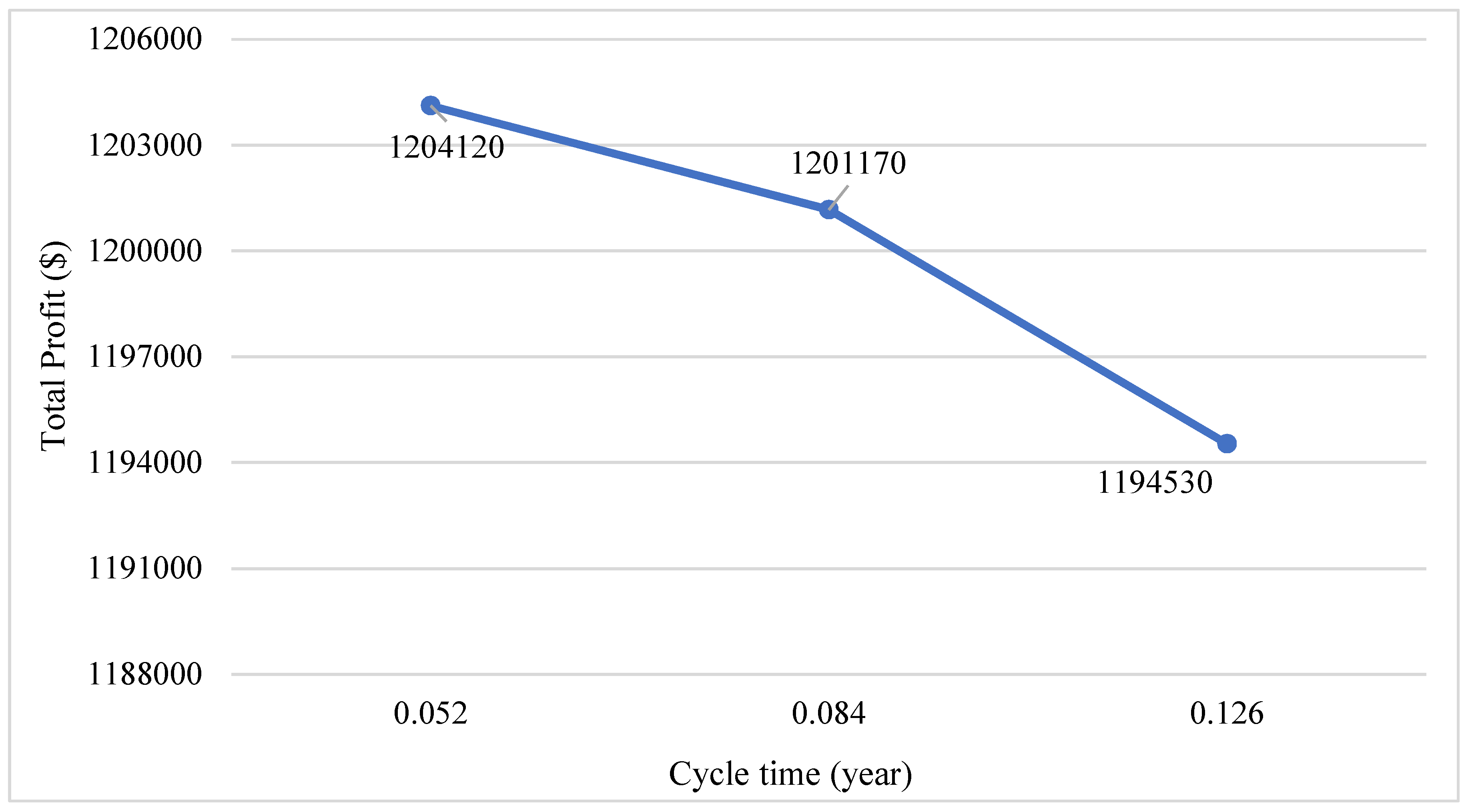
5. Numerical Example

This section of the paper demonstrated the proposed model by showing the numerical solution of the following example. The numerical data for the given example is written in Table 2. This numerical data is taken from Taleizadeh et al. (2016a) with the additional parameters of u, w, l, N, M, Ie, Ic1, and Ic2. The optimal results for all three cases for the total profit and decision variables are shown in Table 3. Figure 6 presents the graphical representation of the optimal solution for different scenarios.

Results

The result shows that the optimal approach in Case 1 exists when the cycle time period is T = 0.052 year, the fraction of this cycle time with positive inventory level having F = 0.66%, the quantity to be ordered is 2600 units, and total profit is $1,204,120. In this scenario, cycle time T is smaller or equal to the permissible payment period M given to the buyer by the supplier. For case 2, the optimal policy is achieved when cycle time period is T = 0.084 year, the fraction of this cycle time with positive inventory level having F = 0.71%, the Q is 4200 units, and TP is $1,201,170. In this situation, cycle time T is bigger than first permissible payment period M and smaller or equal to second permissible payment period N given to the buyer by the supplier. Finally, for Case 3, the optimal policy is achieved when the cycle time period is T = 0.126 year, the fraction of this cycle time with a positive inventory level having F = 0.74%, the quantity to be ordered is 6300 units, and total profit is $1,194,530. In this case, the cycle time T is bigger than both the permissible payment periods M and N given to the buyer by the supplier. From these results, it is clear that highest profit is obtained in Case 3 and lowest profit is obtained in Case 1.
These outcomes illustrate that the total annual profit is lower if the permissible delay payment period given to the buyer by the supplier is larger or equal to the cycle time and more profit is obtained if the permissible delay payment period given to the buyer is smaller than the cycle time. As interest is earned due to this financial aid by selling these items helps the buyer to increase their profit. The optimal result is obtained for the cycle time T by using parameters, whereas the fraction of the cycle time with a positive inventory level F depends upon the cycle time. This must be in the interval of [0, 1]. If F is equal to exactly one, then shortages do not occur. Conversely, if F is equal to zero, then a loss of all demand will occur. The increment in the fraction of backordered demand increases the total profit in all cases, as shown in Figure 7. Additionally, it is also notable, as shown in Figure 8, that due to an increment in the value of the unit holding cost, the total profit is decreased in all cases. If the unit holding cost is higher, then the more permissible period for delay-in-payment is not feasible for the optimal solution. Further analysis of the total profit by changing the various input parameters are shown in the next section.

6. Sensitivity Analysis

This section further analyzes the effect of changes in several key parameters h, π, γ, ct, clm, w, Ie, Ic1, Ic2, M, and N on the total profit per unit for all cases TC (T,F). The sensitivity study of the said parameters for the proposed model on the basis of the given example for different scenarios are given in Table 4. Figure 7, Figure 8 and Figure 9 shows the graphical presentation of some key parameters. The following results are achieved:
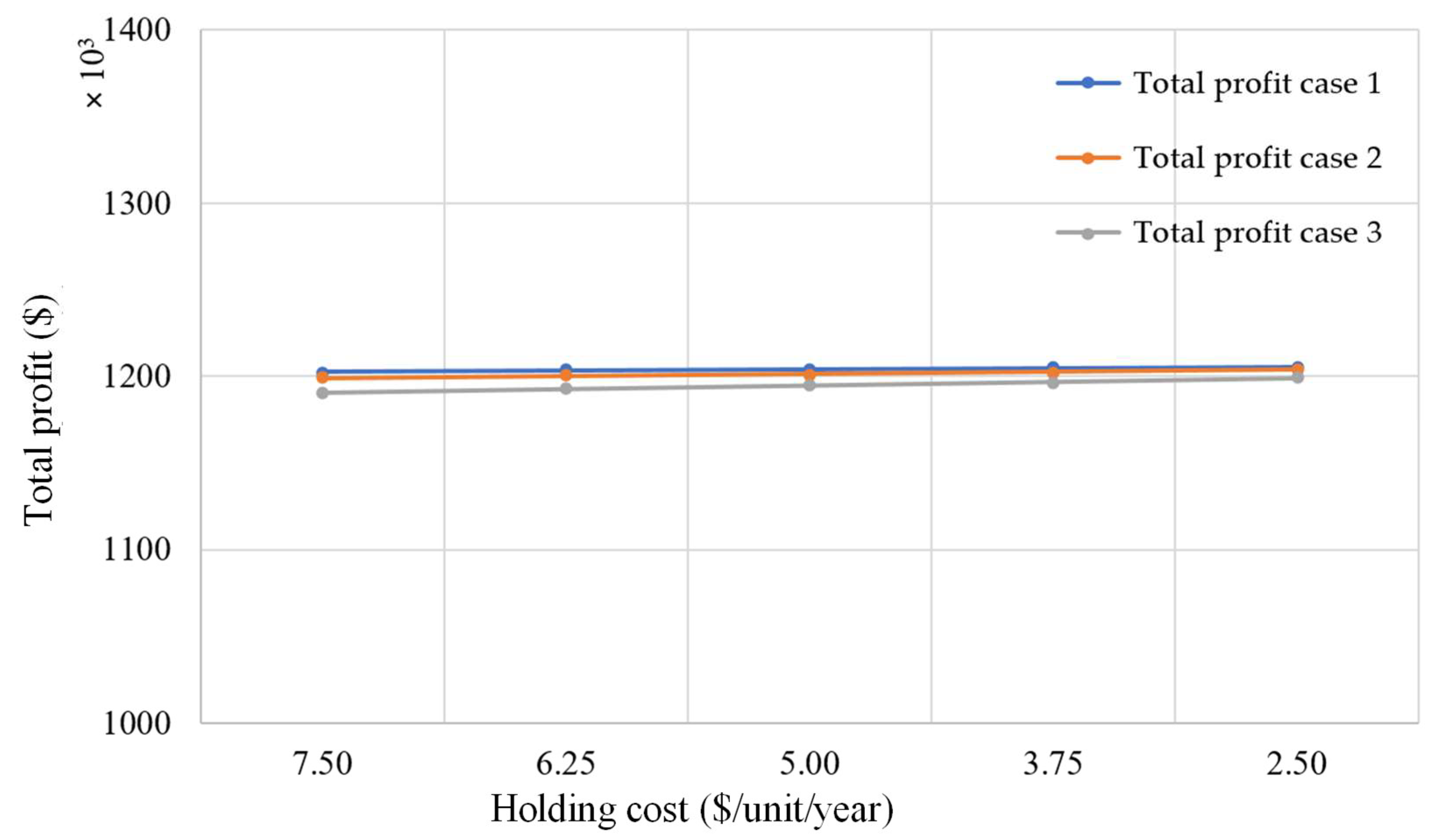
  • Change in a parameter value of holding cost h causes a minor change in total profit for all scenarios. Furthermore, an increment in the value of h by 25% and 50% creates a decrease in TP of 0.11% and 0.06% for Case 1, decreases of 0.10% and 0.21% for Case 2, and decreases of 0.17% and 0.34% for Case 3, respectively. Similarly, a decrement in the value of h by 25% and 50% creates a total profit increase by 0.06% and 0.06% for Case 1, increases of by 0.10% and 0.21% for Case 2, and increases of 0.17% and 0.34% for Case 3, respectively. This shows that there an equilibrium point exists. Also, it illustrates that TP is equally sensitive to both negative and positive changes of parameter h.
  • The outcome of a parameter change in the backorder cost π creates a minor change in total profit for all cases. Though, the increment in the value of π by 25% and 50% causes a decrease in each case. Similarly, for a decrement in the value of parameter π by both 25% and 50%, the total profit increases. It is valuable to state that it lies in an equilibrium state. Also, TP is equally sensitive to both negative and positive changes of parameter π.
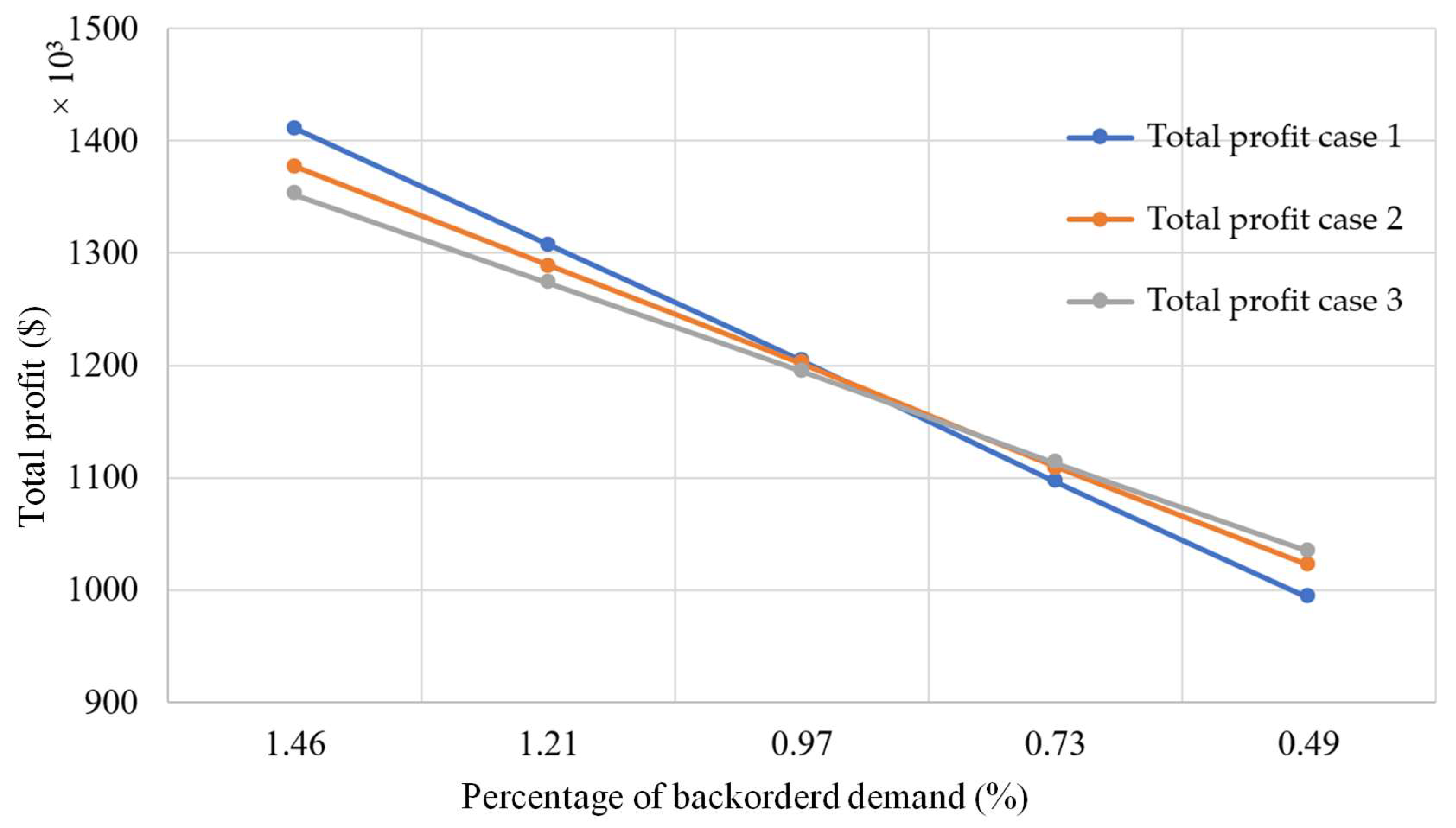
  • The result of a parameter change in the fraction of backorder demand γ causes a major change in the total profit for different cases. Moreover, an increment in the value of γ by 25% and 50% causes an increase in TP by 8.58%, 7.31%, and 6.57%, and 17.16%, 14.63%, and 13.14% for Case 1, Case 2, and Case 3, respectively. Likewise, for a decrement in the value of parameter γ by 25% and 50%, the total profit decreases by 8.93%, 7.62%, and 6.84%, and 17.51%, 14.93%, and 13.42% for Case 1, Case 2, and Case 3, respectively. This does not lie in an equilibrium position. Also, it shows that TP is equally sensitive to both negative and positive change of the parameter γ.
  • The fixed transportation cost of the imperfect item for repair shops cT causes a minor change in total profit for all cases. Furthermore, the increment in the value of cT by 25% and 50% causes a decrease in TP. Similarly, a decrement in the value of parameter cT by 25% and 50%, decreases the total profit. It is exists in an equilibrium position and also total profit is equally sensitive to both negative and positive change of the parameter cT.
  • The labor and material cost for repair shops clm causes a minor change in total profit for all cases. The increment in the value of parameter cT by 25% and 50% causes a decrease in the total profit for each case. Similarly, a decrement in the value of cT by 25% and 50% causes a decrease in the total profit. It also exists in an equilibrium state.
  • The percentage of the return of imperfect items w causes a small change in annual profit in all three cases. If the value of w is increased by 25% and 50%, then TP decreases for all cases. Similarly, if we decrease the said parameter by 25% and 50%, the annual total profit increases for each case. Therefore, the change in the parameter causes an inverse change in annual total profit but this lies in an equilibrium position.
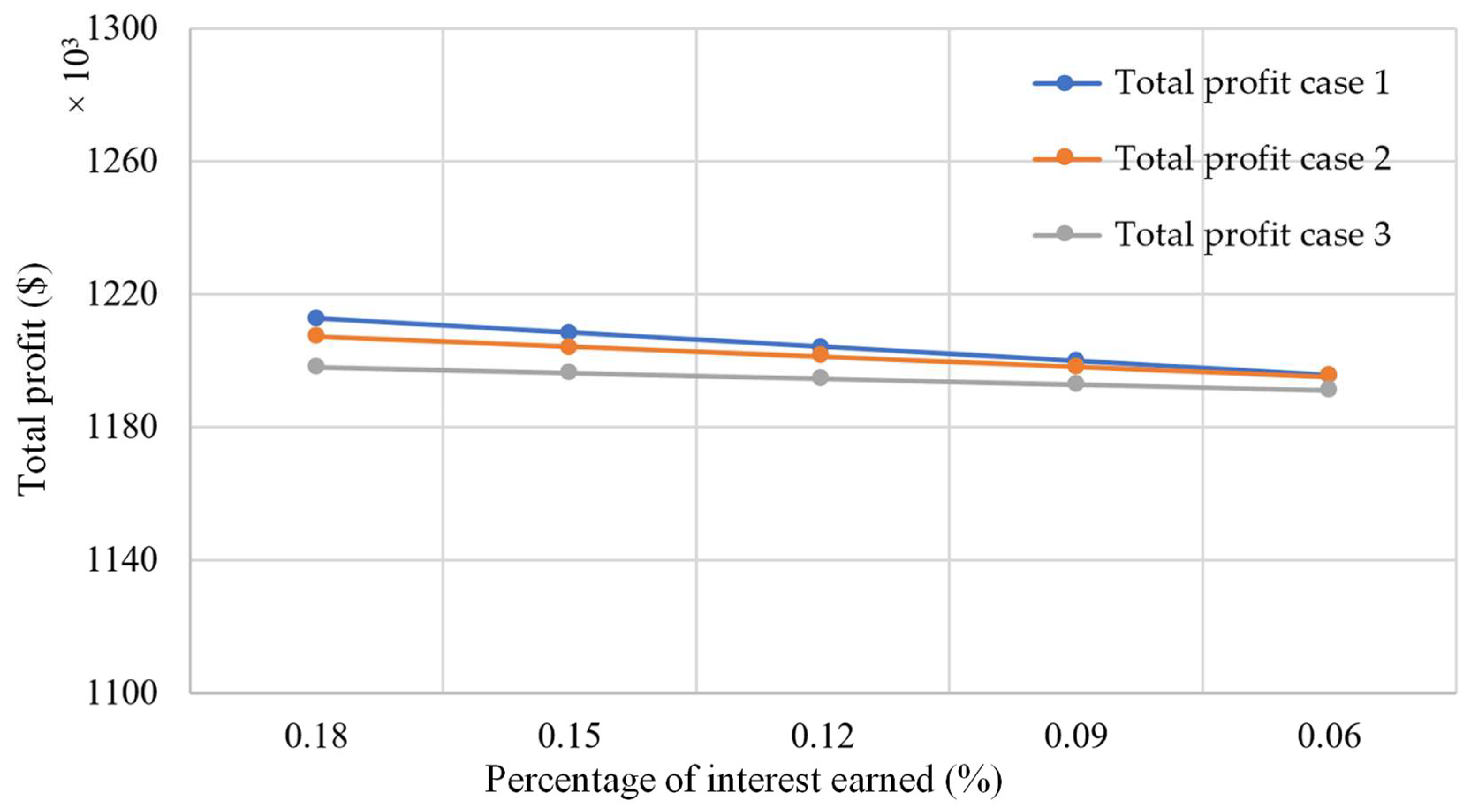
  • The outcome of a parameter change in the interest earned per dollar per year Ie causes a minor change in total profit for each case. Additionally, if the value of Ie is increased by 25% and 50%, then total profit also increases for all cases. Similarly, a decrement in the value of parameter Ie by 25% and 50% causes a decrease in total profit. The result shows that total profit is closely related to interest earned and it also exists in an equilibrium state.
  • The result of a parameter change in interest charged Ic1 and Ic2 are not applicable to Case 1, as no interest is charged for this case. Also, Ic2 is not applicable to Case 2, as no interest rate Ic2 is charged for this case. For Case 2 and Case 3, Ic1 causes a minor change in total profit. Additionally, if the value of Ic1 is increased by 25% and 50%, then total profit increases for both cases. Similarly, if we decrease the parameter Ic1 by 25% and 50%, the annual total profit decreases. A similar pattern is shown for parameter Ic2 in Case 3. An equilibrium position also exists in their patterns.
  • The first permissible delay period M causes a marginal change in annual total profit for Case 1 and Case 2 only. The incremental change in this parameter by 25% and 50% causes an increase in total profit for Case 1, but in contrast for Case 2 with an increase in 50 % of this parameter, the total profit is decreased. For a 25% increment in the parameter, Case 2 shows a similar pattern as Case 1. On the other hand, a decrease in parameter M by 25% and 50% causes a decrease in total profit for both cases.
  • The second permissible delay period N causes a change in total profit for Case 2 and Case 3 only. The Case 1 has no concern with it. The incremental change in this parameter by 25% causes an increase in total profit for both cases, but in contrast by increasing 50% and also by decreasing 25% and 50%, the total profit is decreased in both cases.

7. Managerial Insights

This paper demonstrates key and deliberate insights for managers who need to consider imperfect items, reparation of the defective items, and multi-trade-credit policy. The selection of a scenario in which the cycle time is larger than both the first and second permissible delay payment period given by the supplier to buyer gives the maximum total profit. The industrial managers have to make a judgment on the reasoning of the cycle time and a fraction of the time with a positive inventory level. There must be a tradeoff between these parameters in order to achieve a win-win situation. This study also shows a deep sensitivity analysis for managers on total profit by changing the main input parameters, such as unit holding cost, backorder demand, interest earned, interest paid, transportation cost of imperfect items, and material cost for repair shop, on the numerical setting.
Additionally, this study shows a path towards coping with imperfect items if the supplier is located far away. These imperfect items are still valuable and can be repairable. To get more profit, managers should focus on their cycle time, a fraction of backordered demand, and permissible delay payment period strategies. The manager must decide whether to increase the sales and how much permissible delay-in-payment should be taken to reduce the inventory in stock. In order to maximize profit further in the practices, the industrial managers must give more focused attention on controlling key parameters by thoroughly understanding the relations as shown in the sensitivity analysis. In brief, the result and analysis of this research provide a guideline to help industrial decision-makers to make optimal profits.

8. Conclusions

This paper studied the sustainable inventory model with synergic effects of reworking for imperfect products for environmental impact with the integration of backordering and multi-delay-in-payment. Additionally, the cost of carbon emission is also incorporated in the model to elaborate on the environmental impact in the profit function. In this paper, a situation is created in which supplier is located far away from the buyer. The production system of the supplier may not manufacture all perfect items. Furthermore, there is a chance that the stock received by the buyer has imperfect items. Due to the distant location of the supplier, it is impossible for the buyer to send back these imperfect items at once. The imperfect items have a value and can be repairable in less time, which is sustainable and saves a negative impact on the environment and cost as compared to the high exchange cost and time to exchange with the supplier. In such a circumstance, this study makes an extension of the inventory model with imperfect items, sustainable reparation of these items in the local shop to reduce environmental concerns, and partial backordering. These imperfect products can be taken out of inventory as soon as the screening process is completed and shipped to a local repair shop as a single lot. After completion of the rework, the products are carried back to the buyer. The rework products are returned back to the buyer when the initial inventory level reaches to zero. The inventory system was also synchronized with a trade credit strategy in terms of multi-delay-in-payment. This multi-delay-in-payment acts as a source of interim financial investment and it can be used to increase the sales. The optimal solution according to different scenarios of the cycle time with permissible delay-in-payment is derived. The non-derivative method is used in the proposed study to accomplish an optimal solution of the proposed model at hand. This approach has been verified confidently in previous inventory models. Finally, we illustrate a numerical example to express the developed inventory model and draw a sensitivity analysis of the main input parameters.
In this research, we tried to exploit structural properties of the total profit function by making a payment with multi-trade-credit policy and practices to produce theoretical outcomes. The integration of a carbon emission cost in the total profit function also elaborates the sustainable inventory models and literature. The joint understanding among business members was used to get the optimal total profit. The study also has impacts on firm financing. The industrial managers should decide how much reconciliation can be created to exercise this policy for profit maximization. If the initial unit holding cost of perfect products is higher, then the larger permissible period for delay-in-payment is not feasible to get the optimal solution. This model can help in making decisions to enhance the performance of sustainable inventory management by controlling cycle time and a fraction of time for a global supply chain under partial backordering and a multi-trade-credit-period. Future research might be carried out in many directions. Future work that researchers can cover is a reform of this model with a multi-buyer and multi-product case. The incorporation of carbon emission costs in the transportation sector and production processes in these models is also a promising opportunity for future study.

Author Contributions

Conceptualization, W.A.; software, M.T.; methodology, funding acquisition, validation, writing—review and editing, data curation, project administration, resources, writing—original draft preparation, supervision, B.S.; visualization, formal analysis, investigation, S.-B.C.

Funding

There was no funding for this paper.

Conflicts of Interest

The authors declare no conflict of interest.

Appendix A

Optimal values of F* and T* for Case 2:
The profit function for Case 2 in Equation (13), found by adding +1 and −1 in order quantity is given as:
T P ( F , T ) = P D ( 1 ( 1 F ) ( 1 γ ) [ O T + C u D ( 1 ( 1 F ) ( 1 γ ) ) + C s F D + ( h + h ) [ ( 1 β ) 2 F 2 T D 2 + β T ( F D ) 2 x ] + ( h r + h r ) [ ( β F ) 2 T D 2 ] + π ( 1 F ) 2 γ T D 2 + β F D ( 1 + m ) [ s r + 2 A β F T D + c l m + 2 c t + ( h s + h s ) ( β F T D R + t T ) ] + l ( 1 γ ) ( 1 F ) D + ( u + g ) w F D + P I e ( D M ) 2 2 T D C u I c 1 ( T D D M ) 2 2 T D ]
Rearranging the terms gives:
T P ( F , T ) = P D C u D [ O T + C s F D + ( h + h ) [ ( 1 β ) 2 F 2 T D 2 + β T ( F D ) 2 x ] + ( h r + h r ) [ ( β F ) 2 T D 2 ] + π ( 1 F ) 2 γ T D 2 + β F D ( 1 + m ) [ s r + 2 A β F T D + c l m + 2 c t + ( h s + h s ) ( β F T D R + t T ) ] + l ( 1 γ ) ( 1 F ) D + ( u + g ) w F D + P I e ( D M ) 2 2 T D C u I c 1 ( T D D M ) 2 2 T D + P D ( ( 1 ( 1 F ) ( 1 γ ) ) C u D ( ( 1 ( 1 F ) ( 1 γ ) ) ]
By putting C z = ( P + g C u ) , then the total profit function becomes:
T P ( F , T ) = D ( P C u ) [ O T + C s F D + ( h + h ) [ ( 1 β ) 2 F 2 T D 2 + β T ( F D ) 2 x ] + ( h r + h r ) [ ( β F ) 2 T D 2 ] + π ( 1 F ) 2 γ T D 2 + β F D ( 1 + m ) [ s r + 2 A β F T D + c l m + 2 c t + ( h s + h s ) ( β F T D R + t T ) ] + ( u + g ) w F D + P I e ( D M ) 2 2 T D C u I c 1 ( T D D M ) 2 2 T D + C z D ( ( 1 ( 1 F ) ( 1 γ ) ) ]
The profit function can be further simplified to:
T P ( F , T ) = D ( P C u ) C u I c 1 D M C z D ( 1 γ ) [ 1 T ( O + ( 1 + m ) ( s r + 2 A ) P I e D M 2 2 + C u I c 1 D M 2 2 + F ( C s D + β D ( 1 + m ) [ c l m + 2 c t + ( h s + h s ) t T ] C z D ( 1 γ ) ) + T ( π γ D 2 + C r I c 1 D 2 ) F T ( γ π D ) + F 2 T ( ( 1 + m ) ( h s + h s ) β 2 D 2 R + ( 1 β ) 2 ( h + h ) D 2 + β ( h + h ) D 2 x + ( h r + h r ) β 2 D 2 + π γ D 2 ) ]
as the D ( P C u ) C z D ( 1 γ ) C u I c 1 D M terms are constant. The total profit per year is maximized if total cost per year is minimized. Therefore, the Y(F,T) is:
Y ( F , T ) = [ 1 T ( O + ( 1 + m ) ( s r + 2 A ) P I e D M 2 2 + C u I c 1 D M 2 2 F ( C s D + β D ( 1 + m ) [ c l m + 2 c t + ( h s + h s ) t T ] C z D ( 1 γ ) ) + T ( π γ D 2 + C r I c 1 D 2 ) + F T ( γ π D ) + F 2 T ( ( 1 + m ) ( h s + h s ) β 2 D 2 R + ( 1 β ) 2 ( h + h ) D 2 + β ( h + h ) D 2 x + ( h r + h r ) β 2 D 2 + π γ D 2 ) ]
The compact form of Y(F,T) can be expressed as:
Y ( F , T ) = 1 T ( J 1 ) + T ( J 2 J 4 F + J 5 F 2 ) + J 3 F
(see Appendix D for all values).
We can re-write Equation (A6) as:
Y ( F , T ) = 1 T ( J 1 ) + T λ ( F ) + α ( F )
where λ ( F ) = J 2 J 4 F + J 5 F 2 and α ( F ) = J 3 F .
The total cost equation reaches the lowest value with respect to T when:
T * = J 1 λ ( F )
The minimum value for the total cost by substituting T* in the cost equation is:
Y ( F ) = 2 J 1 λ ( F ) + α ( F )
The optimal T* depends upon F. An algebraic approach is used to get the optimal values of F. Now, the model takes only that part of the equation that consists of the decision variables. The optimal value of F is given as:
F * = J 4 T J 3 2 J 5 T
By putting the values of J4, J3, and J5 in Equation (A10):
F * = π γ T ( C s + β ( 1 + m ) ( c l m + 2 c t + ( h s + h s ) t T ) C z ( 1 γ ) [ 2 ( 1 + m ) ( h s + h s ) β 2 D R + ( 1 β ) 2 ( h + h ) + 2 β ( h + h ) D x + ( h r + h r ) β 2 + π γ ] T
From Equation (A8):
T * = J 1 J 2 J 4 F + J 5 F 2
Putting the optimum value of F in Equation (A12) gives:
T * = J 1 J 2 J 4 ( J 4 T J 3 2 J 5 T ) + J 5 ( J 4 T J 3 2 J 5 T ) 2
Finally, putting the values of J1, J2, J3, J4, and J5 in Equation (A12) gives:
T * = ( O + ( 1 + m ) ( s r + 2 A ) + C u I c 1 D M 2 2 P I e D M 2 2 ) ( ( 1 + m ) ( h s + h s ) β 2 D R + ( 1 β ) 2 ( h + h ) 2 + β ( h + h ) D x + ( h r + h r ) β 2 2 + π γ 2 ) D 4 ( C s + β D ( 1 + m ) [ c l m + 2 c t + ( h s + h s ) t T ] C z ( 1 γ ) ) ( π γ 2 + C r I c 1 2 ) ( ( 1 + m ) ( h s + h s ) β 2 D 2 R + ( 1 β ) 2 ( h + h ) D 2 + β ( h + h ) D 2 x + ( h r + h r ) β 2 D 2 + π γ D 2 ) ( π γ ) 2 D 4

Appendix B

Optimal values of F* and T* for Case 3:
The profit function for Case 3 in Equation (14), found by adding +1 and −1 in order quantity, is given as:
T P ( F , T ) = P D ( 1 ( 1 F ) ( 1 γ ) [ O T + C u D ( 1 ( 1 F ) ( 1 γ ) ) + C s F D + ( h + h ) [ ( 1 β ) 2 F 2 T D 2 + β T ( F D ) 2 x ] + ( h r + h r ) [ ( β F ) 2 T D 2 ] + π ( 1 F ) 2 γ T D 2 + β F D ( 1 + m ) [ s r + 2 A β F T D + c l m + 2 c t + ( h s + h s ) ( β F T D R + t T ) ] + l ( 1 γ ) ( 1 F ) D + ( u + g ) w F D + P I e ( D M ) 2 2 T D C u I c 2 ( T D D N ) 2 2 T D C u I c 1 D T ( N T N 2 M T + M N ) C u I c 1 D ( N M ) 2 2 T ]
Rearranging the terms gives:
T P ( F , T ) = P D C u D [ O T + C s F D + ( h + h ) [ ( 1 β ) 2 F 2 T D 2 + β T ( F D ) 2 x ] + ( h r + h r ) [ ( β F ) 2 T D 2 ] + π ( 1 F ) 2 γ T D 2 + β F D ( 1 + m ) [ s r + 2 A β F T D + c l m + 2 c t + ( h s + h s ) ( β F T D R + t T ) ] + l ( 1 γ ) ( 1 F ) D + ( u + g ) w F D + P I e ( D M ) 2 2 T D C u I c 2 ( T D D N ) 2 2 T D C u I c 1 D T ( N T N 2 M T + M N ) C u I c 1 D ( N M ) 2 2 T + P D ( ( 1 ( 1 F ) ( 1 γ ) ) C u D ( ( 1 ( 1 F ) ( 1 γ ) ) ]
By substituting in C z = ( P + g C u ) , the total profit function becomes:
T P ( F , T ) = D ( P C u ) [ O T + C s F D + ( h + h ) [ ( 1 β ) 2 F 2 T D 2 + β T ( F D ) 2 x ] + ( h r + h r ) [ ( β F ) 2 T D 2 ] + π ( 1 F ) 2 γ T D 2 + β F D ( 1 + m ) [ s r + 2 A β F T D + c l m + 2 c t + ( h s + h s ) ( β F T D R + t T ) ] + ( u + g ) w F D + P I e ( D M ) 2 2 T D C u I c 2 ( T D D N ) 2 2 T D C u I c 1 D T ( N T N 2 M T + M N ) C u I c 1 D ( N M ) 2 2 D + C z D ( ( 1 ( 1 F ) ( 1 γ ) ) ]
The profit function can be further simplified to:
T P ( F , T ) = D ( P C u ) C z D ( 1 γ ) C u I c 2 D N + C u I c 1 D N C u I c 1 D M [ 1 T ( O + ( 1 + m ) ( s r + 2 A ) + C u I c 2 D N 2 2 P I e D M 2 2 C u I c 1 D N 2 + C u I c 1 D M N + C u I c 1 D ( N M ) 2 2 + F ( C s D + β D ( 1 + m ) [ c l m + 2 c t + ( h s + h s ) t T ] C z D ( 1 γ ) ) + T ( π γ D 2 + C r I c 2 D 2 ) + F T ( γ π D ) + F 2 T ( ( 1 + m ) ( h s + h s ) β 2 D 2 R + ( 1 β ) 2 ( h + h ) D 2 + β ( h + h ) D 2 x + ( h r + h r ) β 2 D 2 + π γ D 2 ) ]
as the D ( P C u ) C z D ( 1 γ ) C u I c 2 D N + C u I c 1 D N C u I c 1 D M terms are constant. The total profit per year is maximized if total cost per year is minimized. Therefore, the Y (T, F) is:
Y ( F , T ) = [ 1 T ( O + ( 1 + m ) ( s r + 2 A ) + F ( C s D + β D ( 1 + m ) [ c l m + 2 c t + ( h s + h s ) t T ] C z D ( 1 γ ) ) + T ( π γ 2 + P I e 2 ) + F T ( γ π D ) + F 2 T ( ( 1 + m ) ( h s + h s ) β 2 D 2 R + ( 1 β ) 2 ( h + h ) D 2 + β ( h + h ) D 2 x + ( h r + h r ) β 2 D 2 + π γ D 2 ) ]
The compact form of Y(F,T) can be expressed as:
Y ( F , T ) = 1 T ( J 1 ) + T ( J 2 J 4 F + J 5 F 2 ) + J 3 F
(see Appendix E for all values).
We can re-write Equation (B6) as:
Y ( F , T ) = 1 T ( J 1 ) + T λ ( F ) + α ( F )
where λ ( F ) = 1 T ( J 1 ) + J 2 J 4 F + J 5 F 2 and α ( F ) = J 3 F .
The total cost equation reaches a minimum with respect to T when:
T * = J 1 λ ( F )
The minimum value for the total cost by substituting T* in the cost equation is:
Y ( F ) = 2 J 1 λ ( F ) + α ( F )
The optimal T* depends upon F. The algebraic method is used to get the optimal values of F. Now, the model takes only that part of the equation that consists of the decision variables. The optimal value of F is given as:
F * = J 4 T J 3 2 J 5 T
By putting the values of J4, J3, and J5 in Equation (A24):
F * = π γ T ( C s + β ( 1 + m ) ( c l m + 2 c t + ( h s + h s ) t T ) C z ( 1 γ ) [ 2 ( 1 + m ) ( h s + h s ) β 2 D R + ( 1 β ) 2 ( h + h ) + 2 β ( h + h ) D x + ( h r + h r ) β 2 + π γ ] T
From Equation (B8):
T * = J 1 J 2 J 4 F + J 5 F 2
Putting the optimal value of F in Equation (B12) gives:
T * = J 1 J 2 J 4 ( J 4 T J 3 2 J 5 T ) + J 5 ( J 4 T J 3 2 J 5 T ) 2
Finally, by putting the values of J1, J2, J3, J4, and J5 in Equation (B12):
T * = ( O + ( 1 + m ) ( s r + 2 A ) + C u I c 2 D N 2 2 P I e D M 2 2 C u I c 1 D N 2 + C u I c 1 D M N + C u I c 1 D ( N M ) 2 2 ) ( ( 1 + m ) ( h s + h s ) β 2 D R + ( 1 β ) 2 ( h + h ) 2 + β ( h + h ) D x + ( h r + h r ) β 2 2 + π γ 2 ) D 4 ( C s + β D ( 1 + m ) [ c l m + 2 c t + ( h s + h s ) t T ] C z ( 1 γ ) ) 2 ( π γ 2 + C r I c 2 2 ) ( ( 1 + m ) ( h s + h s ) β 2 D 2 R + ( 1 β ) 2 ( h + h ) D 2 + β ( h + h ) D 2 x + ( h r + h r ) β 2 D 2 + π γ D 2 ) ( π γ ) 2 D 4

Appendix C

J 1 = O + ( 1 + m ) ( s r + 2 A ) J 2 = π γ D 2 + P I e D 2 J 3 = C s D + β D ( 1 + m ) [ c l m + 2 c t + ( h s + h s ) t T ] C z D ( 1 γ ) J 4 = π γ D J 5 = ( 1 + m ) ( h s + h s ) β 2 D 2 R + ( 1 β ) 2 ( h + h ) D 2 + β ( h + h ) D 2 x + ( h r + h r ) β 2 D 2 + π γ D 2

Appendix D

J 1 = O + ( 1 + m ) ( s r + 2 A ) P I e D M 2 2 + C u I c 1 D M 2 2 J 2 = π γ D 2 + C r I c 1 D 2 J 3 = C s D + β D ( 1 + m ) [ c l m + 2 c t + ( h s + h s ) t T ] C z D ( 1 γ ) J 4 = π γ D J 5 = ( 1 + m ) ( h s + h s ) β 2 D 2 R + ( 1 β ) 2 ( h + h ) D 2 + β ( h + h ) D 2 x + ( h r + h r ) β 2 D 2 + π γ D 2

Appendix E

J 1 = O + ( 1 + m ) ( s r + 2 A ) P I e D M 2 2 + C u I c 2 D N 2 2 C u I c 1 D N 2 + C u I c 1 D M N + C u I c 1 D ( N M ) 2 2 J 2 = π γ D 2 + C r I c 2 D 2 J 3 = C s D + β D ( 1 + m ) [ c l m + 2 c t + ( h s + h s ) t T ] C z D ( 1 γ ) J 4 = π γ D J 5 = ( 1 + m ) ( h s + h s ) β 2 D 2 R + ( 1 β ) 2 ( h + h ) D 2 + β ( h + h ) D 2 x + ( h r + h r ) β 2 D 2 + π γ D 2

References

  1. Porteus, E.L. Optimal lot sizing, process quality improvement and setup cost reduction. Oper. Res. 1986, 34, 137–144. [Google Scholar] [CrossRef]
  2. Rosenblatt, M.J.; Lee, H.L. Economic production cycles with imperfect production processes. IIE Trans. 1986, 18, 48–55. [Google Scholar] [CrossRef]
  3. Salameh, M.; Jaber, M. Economic production quantity model for items with imperfect quality. Int. J. Prod. Econ. 2000, 64, 59–64. [Google Scholar] [CrossRef]
  4. Eroglu, A.; Ozdemir, G. An economic order quantity model with defective items and shortages. Int. J. Prod. Econ. 2007, 106, 544–549. [Google Scholar] [CrossRef]
  5. Roy, M.D.; Sana, S.S.; Chaudhuri, K. An economic order quantity model of imperfect quality items with partial backlogging. Int. J. Syst. Sci. 2011, 42, 1409–1419. [Google Scholar] [CrossRef]
  6. Vörös, J. Economic order and production quantity models without constraint on the percentage of defective items. Cent. Eur. J. Oper. Res. 2013, 21, 867–885. [Google Scholar] [CrossRef]
  7. Hsu, J.-T.; Hsu, L.-F. An EOQ model with imperfect quality items, inspection errors, shortage backordering, and sales returns. Int. J. Prod. Econ. 2013, 143, 162–170. [Google Scholar] [CrossRef]
  8. Rad, M.A.; Khoshalhan, F.; Glock, C.H. Optimizing inventory and sales decisions in a two-stage supply chain with imperfect production and backorders. Comput. Ind. Eng. 2014, 74, 219–227. [Google Scholar] [CrossRef]
  9. Kazemi, N.; Abdul-Rashid, S.H.; Ghazilla, R.A.R.; Shekarian, E.; Zanoni, S. Economic order quantity models for items with imperfect quality and emission considerations. Int. J. Syst. Sci. Oper. Logist. 2016, 99–115. [Google Scholar] [CrossRef]
  10. Marchi, B.; Zanoni, S.; Zavanella, L.; Jaber, M. Green supply chain with learning in production and environmental investments. IFAC-PapersOnLine 2018, 51, 1738–1743. [Google Scholar] [CrossRef]
  11. Bazan, E.; Jaber, M.Y.; El Saadany, A.M. Carbon emissions and energy effects on manufacturing–remanufacturing inventory models. Comput. Ind. Eng. 2015, 88, 307–316. [Google Scholar] [CrossRef]
  12. Wahab, M.; Mamun, S.; Ongkunaruk, P. EOQ models for a coordinated two-level international supply chain considering imperfect items and environmental impact. Int. J. Prod. Econ. 2011, 134, 151–158. [Google Scholar] [CrossRef]
  13. Taleizadeh, A.A.; Soleymanfar, V.R.; Govindan, K. Sustainable economic production quantity models for inventory systems with shortage. J. Clean. Prod. 2018, 174, 1011–1020. [Google Scholar] [CrossRef]
  14. Manna, A.; Das, B.; Dey, J.; Mondal, S. Two layers green supply chain imperfect production inventory model under bi-level credit period. Tékhne 2017, 15, 124–142. [Google Scholar] [CrossRef]
  15. Sarkar, B.; Ahmed, W.; Kim, N. Joint effects of variable carbon emission cost and multi-delay-in-payments under single-setup-multiple-delivery policy in a global sustainable supply chain. J. Clean. Prod. 2018, 185, 421–445. [Google Scholar] [CrossRef]
  16. Kim, M.-S.; Sarkar, B. Multi-stage cleaner production process with quality improvement and lead time dependent ordering cost. J. Clean. Prod. 2017, 144, 572–590. [Google Scholar] [CrossRef]
  17. Moshtagh, M.S.; Taleizadeh, A.A. Stochastic integrated manufacturing and remanufacturing model with shortage, rework and quality based return rate in a closed loop supply chain. J. Clean. Prod. 2017, 141, 1548–1573. [Google Scholar] [CrossRef]
  18. Li, D.; Zhao, Y.; Zhang, L.; Chen, X.; Cao, C. Impact of quality management on green innovation. J. Clean. Prod. 2018, 170, 462–470. [Google Scholar] [CrossRef]
  19. Ahmed, W.; Sarkar, B. Impact of carbon emissions in a sustainable supply chain management for a second generation biofuel. J. Clean. Prod. 2018, 186, 807–820. [Google Scholar] [CrossRef]
  20. Younesi, M.; Roghanian, E. A framework for sustainable product design: A hybrid fuzzy approach based on Quality Function Deployment for Environment. J. Clean. Prod. 2015, 108, 385–394. [Google Scholar] [CrossRef]
  21. Skouri, K.; Konstantaras, I.; Lagodimos, A.; Papachristos, S. An EOQ model with backorders and rejection of defective supply batches. Int. J. Prod. Econ. 2014, 155, 148–154. [Google Scholar] [CrossRef]
  22. Chakraborty, T.; Giri, B. Lot sizing in a deteriorating production system under inspections, imperfect maintenance and reworks. Oper. Res. 2014, 14, 29–50. [Google Scholar] [CrossRef]
  23. Sarkar, B.; Cárdenas-Barrón, L.E.; Sarkar, M.; Singgih, M.L. An economic production quantity model with random defective rate, rework process and backorders for a single stage production system. J. Manuf. Syst. 2014, 33, 423–435. [Google Scholar] [CrossRef]
  24. Jaber, M.Y.; Zanoni, S.; Zavanella, L.E. Economic order quantity models for imperfect items with buy and repair options. Int. J. Prod. Econ. 2014, 155, 126–131. [Google Scholar] [CrossRef]
  25. Sharifi, E.; Sobhanallahi, M.A.; Mirzazadeh, A.; Shabani, S. An EOQ model for imperfect quality items with partial backordering under screening errors. Cogent Eng. 2015, 2, 994258. [Google Scholar] [CrossRef]
  26. Taleizadeh, A.A.; Lashgari, M.; Akram, R.; Heydari, J. Imperfect economic production quantity model with upstream trade credit periods linked to raw material order quantity and downstream trade credit periods. Appl. Math. Model. 2016, 40, 8777–8793. [Google Scholar] [CrossRef]
  27. Zhou, Y.; Chen, C.; Li, C.; Zhong, Y. A synergic economic order quantity model with trade credit, shortages, imperfect quality and inspection errors. Appl. Math. Model. 2016, 40, 1012–1028. [Google Scholar] [CrossRef]
  28. Taleizadeh, A.A.; Khanbaglo, M.P.S.; Cárdenas-Barrón, L.E. An EOQ inventory model with partial backordering and reparation of imperfect products. Int. J. Prod. Econ. 2016, 182, 418–434. [Google Scholar] [CrossRef]
  29. Sarkar, B.; Saren, S. Product inspection policy for an imperfect production system with inspection errors and warranty cost. Eur. J. Oper. Res. 2016, 248, 263–271. [Google Scholar] [CrossRef]
  30. Dey, O. A fuzzy random integrated inventory model with imperfect production under optimal vendor investment. Oper. Res. 2017, 1–15. [Google Scholar] [CrossRef]
  31. Kang, C.W.; Ullah, M.; Sarkar, B.; Hussain, I.; Akhtar, R. Impact of random defective rate on lot size focusing work-in-process inventory in manufacturing system. Int. J. Prod. Res. 2017, 55, 1748–1766. [Google Scholar] [CrossRef]
  32. Wuttke, D.A.; Blome, C.; Heese, H.S.; Protopappa-Sieke, M. Supply chain finance: Optimal introduction and adoption decisions. Int. J. Prod. Econ. 2016, 178, 72–81. [Google Scholar] [CrossRef] [Green Version]
  33. Pfohl, H.-C.; Gomm, M. Supply chain finance: Optimizing financial flows in supply chains. Logist. Res. 2009, 1, 149–161. [Google Scholar] [CrossRef]
  34. Goyal, S.K. Economic order quantity under conditions of permissible delay in payments. J. Oper. Res. Soc. 1985, 36, 335–338. [Google Scholar] [CrossRef]
  35. Chand, S.; Ward, J. A note on “Economic order quantity under conditions of permissible delay in payments”. J. Oper. Res. Soc. 1987, 38, 83–84. [Google Scholar]
  36. Shah, N.H. Probabilistic time-scheduling model for an exponentially decaying inventory when delays in payments are permissible. Int. J. Prod. Econ. 1993, 32, 77–82. [Google Scholar] [CrossRef]
  37. Huang, Y.-F. Optimal retailer’s ordering policies in the EOQ model under trade credit financing. J. Oper. Res. Soc. 2003, 54, 1011–1015. [Google Scholar] [CrossRef]
  38. Soni, H.; Shah, N.H. Optimal ordering policy for stock-dependent demand under progressive payment scheme. Eur. J. Oper. Res. 2008, 184, 91–100. [Google Scholar] [CrossRef]
  39. Tsao, Y.-C.; Chen, T.-H.; Zhang, Q.-H. Effects of maintenance policy on an imperfect production system under trade credit. Int. J. Prod. Res. 2013, 51, 1549–1562. [Google Scholar] [CrossRef]
  40. Sana, S.S.; Chedid, J.A.; Navarro, K.S. A three layer supply chain model with multiple suppliers, manufacturers and retailers for multiple items. Appl. Math. Comput. 2014, 229, 139–150. [Google Scholar] [CrossRef]
  41. Yang, M.; Tseng, W.-C. Three-echelon inventory model with permissible delay in payments under controllable lead time and backorder consideration. Math. Probl. Eng. 2014, 2014. [Google Scholar] [CrossRef]
  42. Jaggi, C.K.; Yadavalli, V.; Verma, M.; Sharma, A. An EOQ model with allowable shortage under trade credit in different scenario. Appl. Math. Comput. 2015, 252, 541–551. [Google Scholar] [CrossRef]
  43. Soni, H.N.; Patel, K.A. Optimal strategy for an integrated inventory system involving variable production and defective items under retailer partial trade credit policy. Decis. Support Syst. 2012, 54, 235–247. [Google Scholar] [CrossRef]
  44. Tsao, Y.-C.; Linh, V.T. Supply Chain Network Designs Developed for Deteriorating Items under Conditions of Trade Credit and Partial Backordering. Netw. Spat. Econ. 2016, 16, 933–956. [Google Scholar] [CrossRef]
  45. Giri, B.; Sharma, S. Optimal ordering policy for an inventory system with linearly increasing demand and allowable shortages under two levels trade credit financing. Oper. Res. 2016, 16, 25–50. [Google Scholar] [CrossRef]
  46. Tiwari, S.; Ahmed, W.; Sarkar, B. Multi-item sustainable green production system under trade-credit and partial backordering. J. Clean. Prod. 2018, 204, 82–95. [Google Scholar] [CrossRef]
  47. Tsao, Y.-C.; Zhang, Q.; Fang, H.-P.; Lee, P.-L. Two-tiered pricing and ordering for non-instantaneous deteriorating items under trade credit. Oper. Res. 2017, 1–20. [Google Scholar] [CrossRef]
  48. Banu, A.; Mondal, S.K. Analyzing an inventory model with two-level trade credit period including the effect of customers’ credit on the demand function using q-fuzzy number. Oper. Res. 2018, 1–29. [Google Scholar] [CrossRef]
Figure 1. Inventory diagram of the imperfect quality product and rework inventory system with shortages.
Sustainability 10 04761 g001
Figure 2. Inventory level with imperfect items and the return of reworked items when the inventory reaches zero.
Sustainability 10 04761 g002
Figure 3. Graphical representation of interest charged and interest earned for T ≤ M.
Sustainability 10 04761 g003
Figure 4. Graphical representation of interest charged and interest earned for M <T ≤ N.
Sustainability 10 04761 g004
Figure 5. Graphical representation of interest earned and interest charged for T > N > M.
Sustainability 10 04761 g005
Figure 6. Optimal results of different cases for total profit and decision variables.
Sustainability 10 04761 g006
Figure 7. Analysis of the total profit for cases by changing the fraction of the backordered demand.(γ).
Sustainability 10 04761 g007
Figure 8. Analysis of the total profit for each case by changing unit holding cost (h).
Sustainability 10 04761 g008
Figure 9. Analysis of the total profit for each case by changing percentage of interest earned (Ie).
Sustainability 10 04761 g009
Table 1. Contribution of different authors.
Author (s)Inventory ModelImperfect ProductsBackorderingTrade Credit PolicyReworkSustainabilityMulti Delay-in-Payment
Goyal (1985) [34]
Porteus (1986) [1]
Huang (2003) [37]
Soni and Shah (2008) [38]
Roy et al. (2011) [5]
Soni and Patel (2012) [43]
Sana et al. (2014) [40]
Yang and Tseng (2014) [41]
Sarkar et al. (2014) [23]
Jaber et al. (2014) [24]
Sharifi et al. (2015) [25]
Taleizadeh et al. (2016) [26]
Sarkar and Saren (2016) [29]
Taleizadeh et al. (2016) [28]
Tsao and Linh (2016) [44]
Kim and Sarkar (2017) [16]
Marchi et al. (2018) [10]
Sarkar et al. (2018) [15]
Tiwari et al. (2018) [46]
This Paper
Table 2. Data for the numerical example.
ParameterSymbolValueUnits
Demand rateD50,000units/year
Screening ratex175,200units/year
Repaired rateR50,000units/year
Ordering costO100$/order
Purchase costCu25$/unit
Selling priceP50$/unit
Holding cost of perfect producth4$/unit/year
Holding cost at repair storehs3$/unit/year
Holding cost of rework producthr5$/unit/year
Carbon cost for holding perfect producth’1$/unit/year
Carbon cost at repair store for holding producths1$/unit/year
Carbon cost for holding rework producthr1$/unit/year
Inspection costCs0.5$/unit
Backorder costπ20$/unit/year
Lost sales costl0.5$/unit/year
Fraction of backordered demandγ97%percent
Fixed setup cost of repair storesr100$/setup
Fixed cost (transportation)A200$/trip
Transportation cost per unitct2$/unit
Labor and material cost per unitclm5$/unit
Transport timetT2/220year
Markup percentagem20%percent
Percentage of imperfect itemsβ0.04%percent
Penalty cost from goodwill lossg15$/unit
Return costu3$/unit
Percentage of imperfect items returnedw0.02%percent
First permissible delay periodM30days
Second permissible delay periodN45days
Interest earnedIe12%percent
Interest charged for period MIc113%percent
Interest charged for period NIc220%percent
Table 3. Optimum total cost for Case 1 with different values of decision variables.
ScenarioT (year)F (%)Q (units)TP ($)
Case 10.0520.6626001,204,120
Case 20.0840.7142001,201,170
Case 30.1260.7463001,194,530
Table 4. Sensitivity analysis of the key parameters.
Parameter% Change% Change TP (T,F)
Case 1Case 2Case 3
h+50−0.11−0.21−0.34
+25−0.06−0.10−0.17
−25+0.06+0.10+0.17
−50+0.11+0.21+0.34
π+50−0.12−0.14−0.17
+25−0.06−0.07−0.09
−25+0.06+0.07+0.09
−50+0.12+0.14+0.17
γ+50+17.16+14.63+13.14
+25+8.58+7.31+6.57
−25−8.93−7.62−6.84
−50−17.51−14.93−13.42
ct+50−0.26−0.28−0.29
+25−0.13−0.14−0.15
−25+0.13+0.14+0.15
−50+0.26+0.28+0.29
clm+50−0.33−0.35−0.37
+25−0.16−0.18−0.18
−25+0.16+0.18+0.18
−50+0.33+0.35+0.37
w+50−0.30−0.32−0.33
+25−0.15−0.16−0.17
−25+0.15+0.16+0.17
−50+0.30+0.32+0.33
Ie+50+0.71+0.51+0.29
+25+0.36+0.26+0.15
−25−0.35−0.26−0.15
−50−0.71−0.51−0.29
Ic1+50N/A+0.51+0.29
+25N/A+0.26+0.15
−25N/A−0.26−0.15
−50N/A−0.51−0.29
Ic2+50N/AN/A+0.29
+25N/AN/A+0.15
−25N/AN/A−0.15
−50N/AN/A−0.29
M+50+1.03−0.36N/A
+25+0.52+0.24N/A
−25−0.52−0.31N/A
−50−1.09−0.77N/A
N+50N/A−0.36−0.04
+25N/A+0.24+0.003
−25N/A−0.31−0.03
−50N/A−0.77−0.23

