Development of a Metamodel to Predict Cooling Energy Consumption of HVAC Systems in Office Buildings in Different Climates

Abstract

The use of energy for space cooling is growing faster than any other end use in buildings, justifying the search for improvements in the energy efficiency of these systems. A simplified model to predict cooling energy consumption in Brazilian office buildings was developed. Artificial neural networks (ANNs) were trained from consumption data obtained by building simulation. As it is intended to be applicable to different climates, a new climate indicator also appropriate for hot and humid climates was proposed and validated. The Sobol sensibility analysis was performed to reduce the number of input factors and thus the number of cases to be simulated. The data was built with the simulation of 250,000 cases in Energyplus. Studies were conducted to define the sample size to be used for the ANN training, as well as to define the best ANN architecture. The developed metamodel was used to predict the consumption of Heating, Ventilating and Air Conditioning (HVAC) system of 66,300 new unseen cases. The results showed that the new proposed climate indicator was more accurate than the usual climate correlations, such as cooling degree hours. The developed metamodel presented good performance when predicting annual HVAC consumption of the cases used to obtain the model (R² = 0.9858 and NRMSE = 0.068) and also of the unseen cases (R² = 0.9789 and NRMSE = 0.064).

1. Introduction

Building energy consumption is growing, and has reached significant values in developed countries. Several factors contribute to the growing energy demand, including population growth, an increased demand for building services, the need for better comfort levels, and greater time spent by occupants inside buildings [1]. The use of energy for space cooling is growing faster than any other end use in buildings; it more than tripled between 1990 and 2016, and could triple again by 2050 [2]. For this reason, an improvement in the energy efficiency of buildings is currently one of the main objectives of energy policies in developed and emerging countries [3].

Elaborated and simplified methods have been proposed to predict building energy consumption. These methods have been applied in the design, operation, and retrofit of buildings in recent years [4,5,6,7]. The variety of methods can be divided into three primary categories: Engineering methods, statistical methods and hybrid methods. The engineering methods (also known as white box methods) use physical principles to calculate thermal dynamics and energy behavior of the building. Several dynamic building simulation softwares have been developed in order to use elaborated engineering methods such as DOE-2, EnergyPlus, BLAST, ESP-r and TRNSYS. Although these simulation tools are effective and accurate, they require many details of the building, its systems, and climate parameters, and these details are generally not available or are difficult to obtain. Another disadvantage is the time required by expert professionals, making evaluations difficult and expensive [5]. The statistical methods (also known as black box methods) are based on the deduction of a function that describes the behavior of a specific system from a relevant database. Additionally, these methods have been regarded as an alternative to the engineering methods, especially for the modeling of existing buildings [8], or during the early stage of architectural design [9], or in the control and operation of the buildings systems [10]. The main techniques used to create statistical models for estimate building energy consumption are multiple linear regression, artificial neural networks (ANN) and support vector machines (SVM). Statistical methods are limited by the fact that they require data, especially in large amounts [4]. In order to overcome the limitations of each previous method, the coupling between them generates hybrid methods or gray box methods.

In building modeling, there are three main strategies of coupling between the engineering and statistical methods. The first strategy uses statistical methods (machine learning) as physical parameters estimator. The second strategy uses statistics (multiple linear regression, ANN or SVM) in order to implement a learning model from data built with an engineering method. The third strategy uses statistical methods in fields where physical models are not effective and accurate enough [4].

In Brazil, the voluntary building energy labelling system for commercial buildings permits the evaluation of a building’s energy efficiency by a simplified or simulation method. The simplified method was developed using the second strategy mentioned above, since multiple linear regression was used with data obtained by simulations of different building sizes and constructive characteristics. Due to its limitations, this method is used to evaluate the envelope’s efficiency, not to predict the energy consumption of the building [11]. Recently, Melo et al. [12] developed a more accurate model to predict the annual cooling energy demand of commercial buildings and, thus, to replace the current method. Again, the model does not predict the energy that the Heating, Ventilating and Air Conditioning (HVAC) system will consume to supply the cooling demand. Reviews regarding prediction of building energy consumption [4,5,6] show that most studies develop models to estimate building energy performance and to predict heating/cooling demand rather than identifying actual consumption. Predicting building energy consumption is not an easy task since it is a function of the building characteristics, the energy systems characteristics, weather parameters, and occupants’ behavior [4]. Methods to include the impacts of occupant behavior have only been recently developed and there are many gaps in knowledge and limitations to current methodologies [13,14,15].

The objective of this research is to develop a hybrid model to predict the cooling energy consumption of HVAC systems in Brazilian office buildings. This study utilizes chilled water HVAC systems. The model consists of training an artificial neural network from consumption data obtained by building simulations of a large number of office buildings. Thus, the research was divided into three phases. In the first phase, a new climate indicator was developed for hot and humid climates. In the second phase, a sensitivity analysis was performed in order to identify the key variables. Simulations of office buildings using the EnergyPlus software were performed to obtain the data. In the third phase, the data were pre-processed to improve the stability of the neural networks training process, and a study was conducted to define the sample size to be used in these training. Then, the artificial neural networks were obtained and a refinement of the metamodel architecture was analyzed. Finally, the model was used to predict HVAC consumption of unseen cases to evaluate its performance.

2. Climate Indicator

The climate is a determining factor in the cooling demand of buildings, as well as in the efficiency of air conditioning equipment. For example, air cooled chillers operate more efficiently at times when the outdoor air temperature is lower. The weather files were used in building simulation while climate correlations were used in simplified methods of building energy prediction. This climate correlations generally used in the literature are heating degree days (HDD) and cooling degree days (CDD). These correlations are calculated from the mean daily dry bulb temperature and are useful where sensible heat is predominant: Cold or dry climates. In hot and humid climates, there is an increase in energy consumption associated with the dehumidification process. Therefore, it is necessary to look for new indicators which also consider the latent heat present in the cooling demand of the building. Huang et al. [16], Sailor et al. [17], Sailor [18], and Krese et al. [19] use the enthalpy latent days (ELD) to incorporate the influence of the latent load. Recent studies have sought to incorporate the influence of both loads (sensitive and latent) on a single climate indicator, either by the use of enthalpy [20] or the use of wet bulb temperature [21,22]. As high humidity is a characteristic of many Brazilian regions, it was necessary to analyze which climate indicator was appropriate to be used in this study, as described below.

2.1. Building Model

The annual cooling demand for a building model was obtained for 20 Brazilian cities using Energyplus software and their respective weather data files in EPW (Energyplus Weather Data) format. Two cities with extreme climates (cold and hot) were initially selected (Curitiba and Manaus), and then 18 other cities were included to represent intermediate climates. The concept of shell and core building was considered for the modeled office buildings, as presented in Figure 1a. A 15-story office building was used as a building model. Each floor was modeled with four perimeter thermal zones and an internal thermal zone, as show in Figure 1b. The perimeter zones were considered as the regions that extend from each facade up to 4.5 m towards the interior of the building (Figure 1b).

Table 1. Characteristics of the model building and HVAC system.

Variable	Value
Dimensions of the typical floor	65 × 18 m
Height between floors	3 m
Number of floors	15
Solar orientation of the building	0°
WWR in the four facades	0.5
Solar factor of glasses	0.82
Thermal transmittance of glasses	5.78 W/m2·K
Solar absorptance of external walls	0.5
Thermal transmittance of external walls	2.6 W/m2·K
Thermal capacity of external walls	156 kJ/m2·K
Solar absorptance of roof	0.3
Thermal transmittance of roof	2.42 W/m2·K
Thermal capacity of roof	253 kJ/m2·K
Thermal capacity of internal walls	60 kJ/m2·K
Air infiltration	0.5 air change per hour
Lighting power density	12.5 W/m2
Equipment power density	16.5 W/m2
Occupancy rate	8.5 m2/person
Daily working hours of weekdays	11 h
Setpoint	24 °C
Economizer/Heat recovery	None/None
Night cycle	Off
Chilled water temperature reset	Off
Ventilation type	Constant Volume
Supply fan delta pressure	450 Pa
Chilled water pump configuration	Constant Primary/Variable Secondary
Chilled water primary pump rated head	179,352 Pa
Chilled water secondary pump rated head	392,400 Pa
Outdoor air flow rate	2.5 L/s·person and 0.3 L/s·m2 floor
Chiller COP	3.0

presents the characteristics of the model building and the HVAC system.

The annual cooling demand for the building was obtained through the sum of the hourly cooling demands on the chiller evaporator (output variable called Chiller Evaporator Cooling Energy in Energyplus). Heating demand was not the focus of this research because it is insignificant in Brazilian office buildings, but cannot be neglected in cold climates

2.2. CDH Calculation

According to McQuiston et al. [23], the degree-day method was the first method developed to estimate heating energy in single-family residential houses, and the procedure was based on the assumption that, on a long-term basis, solar and internal gains for a residential structure will offset heat loss when the mean daily outdoor temperature is 18 °C (base temperature). Therefore, this method considers that the building only needs heating when the outdoor temperature is lower than the base temperature. The calculated fuel consumption is proportional to the difference between the mean daily temperature and the base temperature. Based on this method, which considers that heating energy consumption is directly proportional to the degree-days value, the HDD (heating degree days) climate indicator is internationally used as a climate correction factor in the models for building energy consumption prediction [24]. Analogously, there is the definition of the cooling degree days (CDD) indicator, which allows evaluating the influence of the climate on the building cooling energy consumption, and it is calculated as follows.

$$\mathrm{CDD}=\sum _{\mathrm{n}=1}^{\mathrm{N}}{\left({\overline{\mathrm{t}}}_{\mathrm{o}}-{\mathrm{t}}_{\mathrm{b}}\right)}^{+}$$

(1)

where CDD is the cooling degree days, N is the number of days for the period analyzed, ${\overline{\mathrm{t}}}_{\mathrm{o}}$ is the average daily outdoor temperature, and tb is the base temperature.

The cumulative energy consumption of a building has a linear relationship with the cumulative degree days (adding all the degree days from the first day to the last day for calculation of the energy consumption), as showed by Lin et al. [25] and Lukomshi et al. [26].

The base temperature is set individually for each building, but it is common to use certain values. The ASHRAE (American Society of Heating, Refrigerating and Air-Conditioning Engineers) [27], for example, publishes CDD values for temperatures of 10.0, 18.3, 23.3 and 26.7 °C.

Adopting the same concept of degree days, the climate indicator can also be calculated considering the average temperature of each hour, instead of the average daily temperature. Thus, the cooling degree hours (CDH) is calculated according to the equation below.

$$\mathrm{CDH}=\sum _{\mathrm{n}=1}^{\mathrm{N}}{\left({\mathrm{t}}_{\mathrm{o}}-{\mathrm{t}}_{\mathrm{b}}\right)}^{+}$$

(2)

where CDH is the cooling degree hours, N is the number of hours for the period analyzed, t_o is the average hourly outdoor temperature, and t_b is the base temperature.

The CDH was the first climate indicator analyzed in this research because it better represents the period when the HVAC (Heating Ventilating and Air Conditioning) system is operating than cooling degree days (CDD) [28]; further, the estimation of cooling energy consumption is more accurate. The cooling degree hours (CDH) value for twenty Brazilian cities was calculated. The influence of the choice of the base temperature was evaluated through the use of values between 15 and 22 °C. A linear regression was used to represent the relationship between the annual cooling demand and the corresponding CDH value. The statistical index R² (coefficient of determination) and the standard error were used to evaluate the goodness-of-fit between the predicted value of demand and the value obtained by simulation.

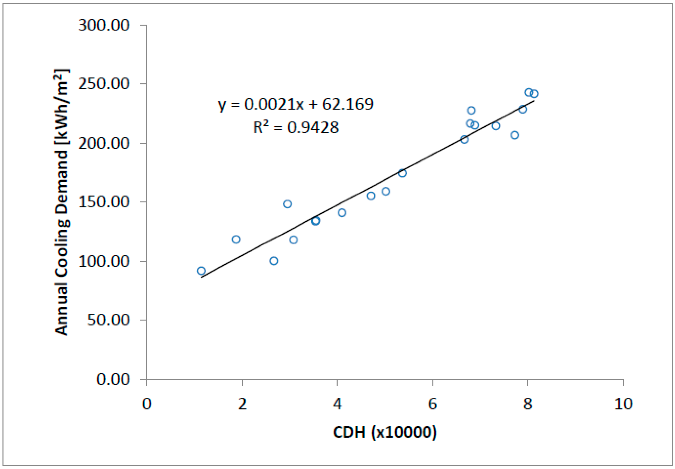
The results of the annual cooling demand for a building model and the CDH indicator (base temperature = 18 °C) are presented in

Table 2. Results for cooling degree hours (CDH) and annual cooling demand for 20 Brazilian cities.

City	CDH	Annual Cooling Demand (kWh/m2·year)
Curitiba	11,401	91.7
Sao Paulo	18,729	118.3
Santa Maria	26,677	100.1
Brasilia	29,493	148.2
Florianopolis	30,758	118.0
Niteroi	35,434	133.7
Belo Horizonte	35,528	134.4
Foz do Iguaçu	40,991	140.9
Rio de Janeiro	47,026	155.2
Campo Grande	50,181	159.1
Governador Valadares	53,655	174.4
Rondonopolis	66,656	202.9
Recife	67,898	216.4
Macapa	68,136	227.6
Salvador	68,881	214.8
Cuiaba	73,252	214.3
Palmas	77,271	206.5
Boa Vista	78,938	228.5
Belem	80,237	242.8
Manaus	81,288	241.6

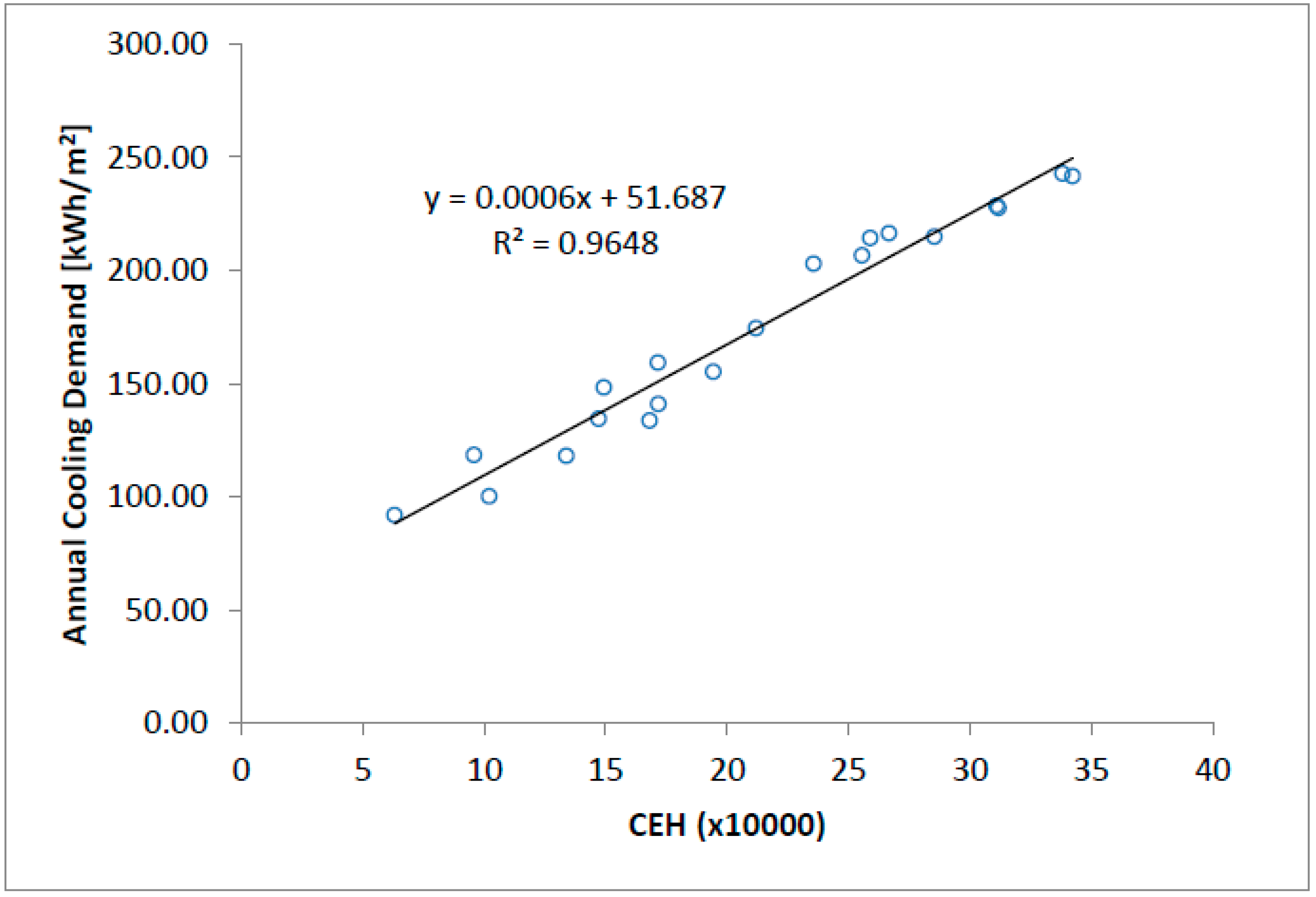
for each of the twenty Brazilian cities analyzed. Figure 2 shows the result of the linear regression used to relate CDH and annual cooling demand. The value obtained for R² was 0.9428, and for the standard error was 12.11 kWh/m²·year.

The CDH was recalculated for different base temperatures to evaluate its influence on the results.

Table 3. Results of the coefficient of determination (R²) obtained with the use of different base temperatures in the CDH.

Base Temperature (°C)	R2
15	0.9360
16	0.9391
17	0.9416
18	0.9428
19	0.9417
20	0.9379
21	0.9301
22	0.9158

presents the value of the coefficient of determination (R²) obtained in each case. The analysis of the results shows that the value of R² did not present significant variation, and the best result was obtained using the base temperature of 18 °C.

2.3. CEH Calculation

Buildings located in regions with hot and humid weather present a large amount of latent load on their cooling demand. Shin and Do [20] used the degrees days method to develop models for energy consumption predictions for two buildings in Texas. Two models were created, one using CDD calculated with dry bulb temperature (CDD_T) according to Equation (1), and the other calculated with enthalpy (CDD_H) according to Equation (3). As a result, the comparison utilizing the enthalpy-based CDD method resulted in a percent error of approximately 2% less than that of the temperature-based CDD method.

$${\mathrm{CDD}}_{\mathrm{H}}=\sum _{\mathrm{n}=1}^{\mathrm{N}}{\left({\overline{\mathrm{h}}}_{\mathrm{o}}-{\mathrm{h}}_{\mathrm{b}}\right)}^{+}$$

(3)

where CDD_H is the enthalpy-based cooling degree days, N is the number of days for the period analyzed, ${\overline{\mathrm{h}}}_{\mathrm{o}}$ is the average daily outdoor enthalpy, and h_b is the base enthalpy.

Considering most Brazilian cities present high values of temperature and humidity, enthalpy was also used in order to create a new climate indicator—called the CEH (Cooling Enthalpy Hours)—Equation (4).

$$\mathrm{CEH} =\sum _{\mathrm{n}=1}^{\mathrm{N}}\propto ·{\left({\mathrm{h}}_{\mathrm{o}}-{\mathrm{h}}_{\mathrm{b}}\right)}^{+}$$

(4)

where CEH is the cooling enthalpy hours, N is the number of hours for the period analyzed, h_o is the average hourly outdoor enthalpy, h_b is the base enthalpy, α = 0 if t < t_b or α = 1 if t ≥ t_b; t is the average hourly outdoor temperature and t_b is the base temperature.

The CEH differs from the CDD_H because it considers the positive differences of enthalpy only when the outdoor temperature is higher than the base temperature. The CEH indicator was calculated for different base enthalpies (values between 34 and 52 kJ/kg), always considering the base temperature of 18 °C.

Table 4. Results of R² obtained with the use of different base enthalpies in the cooling enthalpy hours (CEH).

Base Enthalpy (kJ/kg)	R2
34	0.9647
35	0.9648
36	0.9646
37	0.9643
38	0.9637
39	0.9629
40	0.9619
41	0.9606

presents the value of the coefficient of determination (R²) obtained in each case. For the base enthalpy of 35 kJ/kg, which presented the highest value of R², the standard error of the linear regression was 9.50 kWh/m²·year. Figure 3 shows the linear regression used to relate CEH and annual cooling demand. This result shows that the use of CEH as a climate indicator is more accurate than the use of the traditional CDH indicator.

2.4. CEH Calculation for 407 Brazilian Cities

The new climate indicator CEH and the building model annual cooling demand were calculated for 407 Brazilian cities for which weather files were available. The value of 18 °C was considered for the base temperature and 35 kJ/kg for the base enthalpy. The same procedure was performed considering the definition of Shin and Do [20], but for an hourly basis according to the equation below.

$${\mathrm{CDH}}_{\mathrm{H}} =\sum _{\mathrm{n}=1}^{\mathrm{N}}{\left({\mathrm{h}}_{\mathrm{o}}-{\mathrm{h}}_{\mathrm{b}}\right)}^{+}$$

(5)

where CDH_H is the enthalpy-based cooling degree hours, N is the number of hours for the period analyzed, h_o is the average hourly outdoor enthalpy, h_b is the base enthalpy. A comparison between these two indicators allowed us to evaluate the improvement obtained with the new climate indicator.

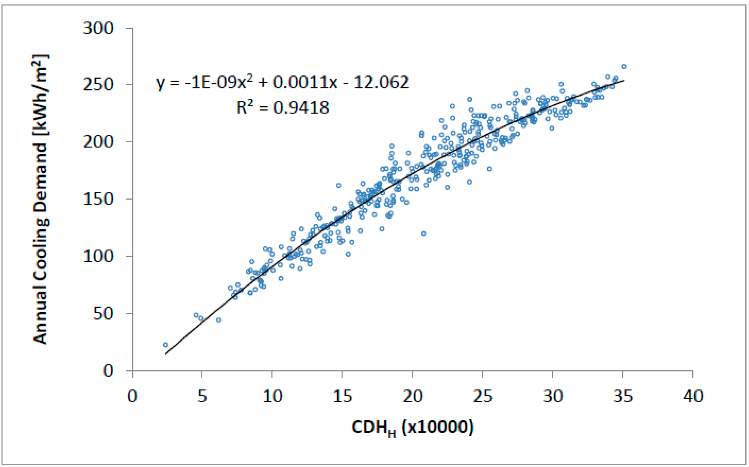
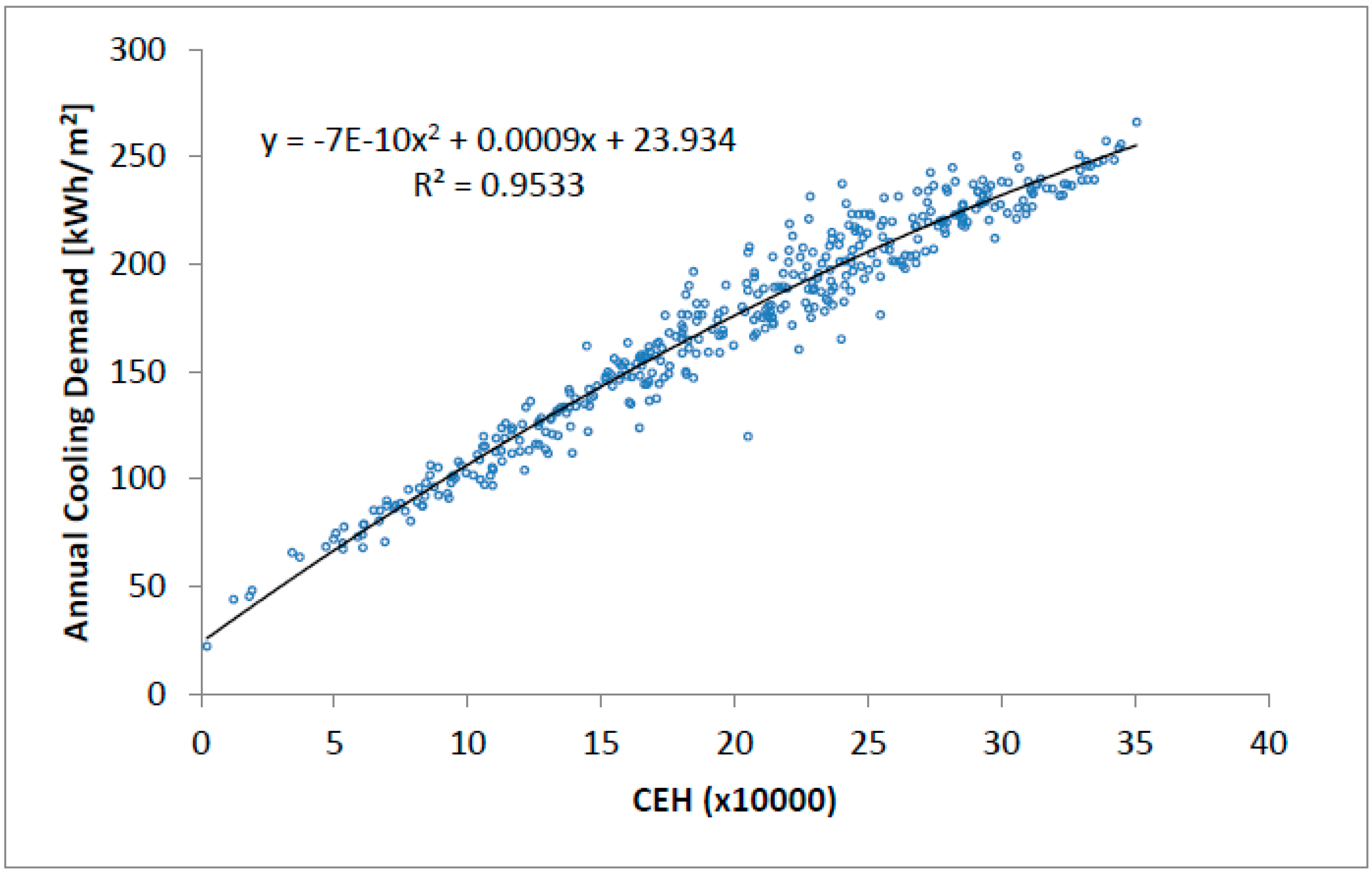
Figure 4 shows the graph that illustrates the correlation between CDH_H and annual cooling demand, where the value obtained for R² was 0.9418, and the standard error was 12.27 kWh/m²·year. Figure 5 shows the correlation between CEH and annual cooling demand, where R² was 0.9533, and the standard error was 11.00 kWh/m²·year.

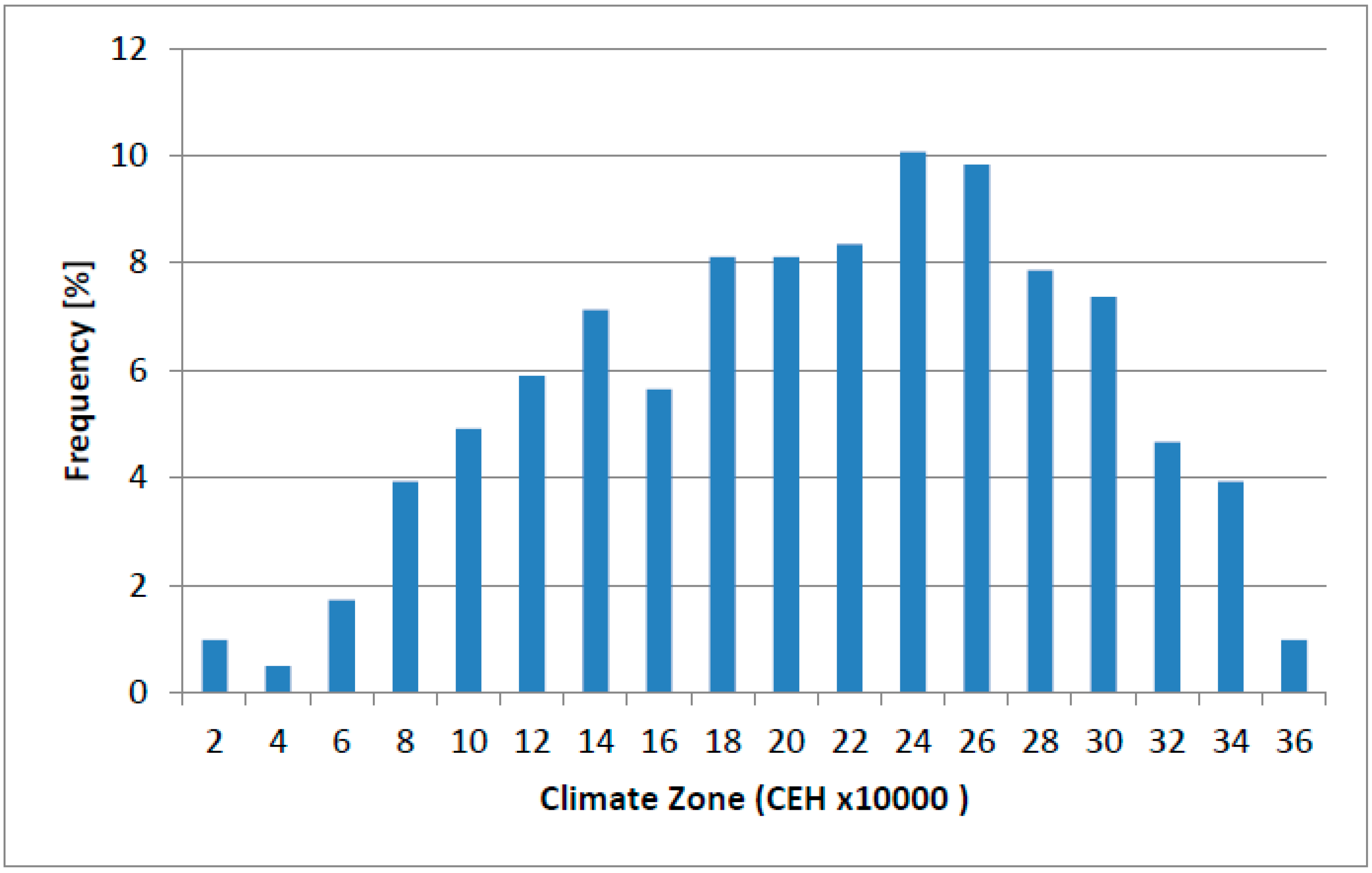
The lowest CEH value calculated for these 407 cities was 2261 and the highest 350,672. Considering groups formed in each interval of 20,000, we obtained 18 climate zones that can be used to characterize the Brazilian climate. A frequency distribution was conducted to verify how each zone was represented from the 407 cities. Figure 6 shows this frequency distribution and Appendix A lists the cities chosen to characterize each of these 18 zones.

2.5. CEH Validation with Other Buildings

The CDH, CDH_H and CEH indicators were also evaluated for buildings other than the building model. The results of 28 new cases were obtained in this research. All buildings are 40-story offices with rectangular geometry and height between floors is equal to 3 m. The external walls have thermal transmittance equal to 2.6 W/m²·K, thermal capacitance of 145 kJ/m²·K, and solar absorptance of 0.4. The internal walls have a thermal capacitance of 145 kJ/m²·K. The roof presents thermal transmittance equal to 1.93 W/m²·K, thermal capacitance of 106 kJ/m²·K, and solar absorptance of 0.5. The setpoint used was 23 °C.

Case 1 is a building with dimensions of 20 × 35 m with the WWR (Windows Wall Ratio) of 25% in the four facades. In Case 1, the vector orthogonal to the length makes an angle of 22.5° with the north, the glass has a solar factor of 0.27 and thermal transmittance of 4.3 W/m²·K, the lighting power density (LPD) is 8.75 W/m², the occupancy rate is 5.0 m²/person, the daily time of operation is 9 h only on weekdays, and the air infiltration rate is 0.37 ACH (air changes per hour). Cases 2–7 are variations of Case 1, where all characteristics are identical except for one. In Case 2 the WWR was changed to 0.65; in Case 3 the solar factor of glass was changed to 0.57; in Case 4 the LPD was changed to 13.75 W/m²; in Case 5 the occupancy rate was changed to 13 m²/person; in Case 6 the daily time of operation was changed to 13 h and, in Case 7 the solar orientation of the building was changed to 112.5°. Cases 8–14 are identical in respective to Cases 1–7 except for their dimensions, 20 × 95 m. Similarly, Cases 15–21 are identical in respective to Cases 1–7 but with dimensions of 40 × 70 m. Finally, Cases 22–28 follow the same logic, where the building has dimensions of 40 × 190 m.

Table 5. The values of R² obtained in the correlation between annual cooling demand and CDH, CDH_H and CEH.

	R2				R2
	CDH	CDHH	CEH		CDH	CDHH	CEH
Case 1	0.9574	0.9730	0.9854	Case 8	0.9089	0.9712	0.9868
Case 2	0.9397	0.9698	0.9825	Case 9	0.9571	0.9777	0.9870
Case 3	0.8299	0.9248	0.9478	Case 10	0.9087	0.9676	0.9827
Case 4	0.9207	0.9667	0.9785	Case 11	0.9285	0.9788	0.9881
Case 5	0.9542	0.9443	0.9672	Case 12	0.9396	0.9599	0.9764
Case 6	0.9316	0.9836	0.9943	Case 13	0.9358	0.9821	0.9934
Case 7	0.9431	0.9682	0.9798	Case 14	0.9105	0.9679	0.9788
Case 15	0.9002	0.9872	0.9926	Case 22	0.9120	0.9867	0.9957
Case 16	0.8902	0.9801	0.9909	Case 23	0.7698	0.9737	0.9906
Case 17	0.9324	0.9810	0.9896	Case 24	0.9052	0.9871	0.9934
Case 18	0.9231	0.9849	0.9920	Case 25	0.9793	0.9994	0.9996
Case 19	0.9411	0.9733	0.9844	Case 26	0.9165	0.9692	0.9851
Case 20	0.7216	0.9853	0.9934	Case 27	0.8915	0.9916	0.9957
Case 21	0.8497	0.9819	0.9887	Case 28	0.9387	0.9929	0.9986

presents the values of R² obtained when a linear correlation between annual cooling demand and each climate indicator is used. These results show that the CEH indicator performs better than the CDH and CDH_H, since the R² value increases 7.8% on average when CDH_H is used in place of CDH and increases 1.1% when CEH is used in the place of CDH_H.

Considering these results, the CEH indicator was chosen to be the climate indicator, and it will be one of the input factors of the artificial neural network to predict energy consumption of HVAC system in office buildings.

3. Data Construction

3.1. Sensitivity Analysis

The objective of this step was to determine the characteristics of the office buildings that, once changed, provide significant changes in their cooling demand, as well as to determine which parameters of the HVAC system have the greatest influence on energy consumption. Thus, only these characteristics and parameters had their values changed to obtain the cases which were simulated to obtain the data. Sensitivity analysis techniques allow evaluating the relative importance of the input factors of a model. These techniques indicate which input factors are most important in determining the uncertainty in the output and if it is possible to keep fixed the values of some input factors of the model.

3.1.1. Input Factors

The building was modeled considering rectangular geometry. The distance between floors was set at three meters. Each floor was modeled with four perimeter thermal zones and an internal thermal zone. The variables used to characterize the geometry were width of building base, ratio between length and width, number of floors, solar orientation and window wall ratio (WWR). The solar factor and thermal transmittance of glasses, the solar absorptance, thermal transmittance and thermal capacity of external walls and roofs, and the thermal capacity of internal walls were the factors used to represent the properties of building materials.

The variables used for heat gains were air infiltration, lighting power density, occupation rate, and daily working hours of weekdays. It was considered that each person dissipates 120 W, where 40% is latent heat and 60% is sensible heat. Dunn and Knight [29] conducted a study in UK offices and demonstrated that there is a strong correlation between the power density of equipment and the occupancy rate. The average value of equipment load obtained by them was 158 W per person. However, due to the continuous growth in the efficiency of office equipment, this value has reduced in recent years. We fit an equation relating occupancy rate and equipment power density from the data presented in Dunn and Knight’s paper [29]. Then, we applied a correction factor of 0.886 in this equation, corresponding to the reduction of the average value of equipment load from 158 to 140 W/m² as verified by Korolija [30], resulting in the following equation.

$$\mathrm{EPD}=116.45·{\left(\mathrm{Occ}\right)}^{-0.923}$$

(6)

where EPD is equipment power density in W/m² and Occ is the occupancy rate in m²/person.

The weather was modeled through the use of 18 weather files which characterize the climate zones defined in the previous step. The HVAC system was modeled with fancoil units in each thermal zone and one chiller. The variables used to characterize the HVAC system were thermostat setpoint temperature, use of economizer, use of heat recovery, use of night cycle, use of chilled water temperature reset, ventilation type, chilled water pump rated head, condenser water pump rated head, outdoor air flow rate, and chiller.

Table 6. Variables and range of values used in the sensibility analysis.

Variable	Range of Values
Width of base of building	10–50 m
Ratio between length and width	1–6
Number of floors	5, 10, 20, 30, 40 or 50
Solar orientation of the building	0–135°
WWR	0.15–0.95
Solar factor of glasses	0.2–0.8
Thermal transmittance of glasses	1.7, 2.7 or 5.8W/m2·K
Solar absorptance of external walls	0.2–0.8
Thermal transmittance of external walls	0.5–2.9 W/m2·K
Thermal capacity of external walls	40–270 kJ/m2·K
Solar absorptance of roof	0.2–0.8
Thermal transmittance of roof	0.5–3.65 W/m2·K
Thermal capacity of roof	30–250 kJ/m2·K
Thermal capacity of internal walls	40–270 kJ/m2·K
Air infiltration	0–0.75 air change per hour
Lighting power density	7.5–17.5 W/m2
Occupancy rate	3–15 m2/person
Daily working hours of weekdays	8, 9, 10, 11, 12, 13, 14, 15 or 16 h
Weather	18 weather files (climate zones)
Setpoint	20–24 °C
Economizer/Heat recovery	Differential Enthalpy/None, or None/Enthalpy, or None/None
Night cycle	Off or On
Chilled water temperature reset	Off or On
Ventilation type	Constant Volume or Variable Volume
Supply fan delta pressure	150–750 Pa
Chilled water pump configuration	Constant Primary/Variable Secondary, or Constant Primary/No Secondary or Variable Primary/No Secondary
Chilled water pump rated head	25–85 × 104 Pa
Condenser water pump rated head	10–65 × 104 Pa
Outdoor air flow rate	Level 1, Level 2 or Level 3
Chiller	10 different chillers (Appendix B)

presents the range of values used for each variable in sensitivity analysis. Some used uniform distribution while others employed discrete. The level 1 for outdoor air flow rate considers 2.5 L/s·person and 0.3 L/s·m²; level 2 considers 3.1 L/s·person and 0.4 L/s·m²; and level 3 considers 3.5 L/s·person and 0.5 L/s·m². The chilled water pump rated head corresponds to the sum of primary and secondary pump rated head. When the system has primary and secondary circuits, the primary pump rated head was considered equal to 150,000 Pa. The characteristics adopted for the chiller were the type of condensation (air or water), the coefficient of performance at full load (COP), and IPLV (Integrated Part Load Value) defined by AHRI (Air Conditioning, Heating and Refrigeration Institute) according to AHRI Standard 550/590. The influence of the chiller on the energy consumption was evaluated with the use of 10 different chillers, whose performance curves were obtained in the Energyplus datasets.

3.1.2. Sensibility Analysis Method

The objective of the sensitivity analysis was to identify which input factors could be maintained with fixed values in the data construction procedure without causing a significant impact on the results. Thus, both the number of cases to be simulated and the computational time were reduced. The most appropriate sensitivity analysis methods for this purpose are variance-based methods [31]. The two commonly used variance-based method are FAST (Fourier Amplitude Sensitivity Test) and Sobol. In this research we opted for the Sobol method because it is more precise, despite being more computationally expensive. Tian [31] reviewed the use of sensitivity analysis methods in building energy analysis and recommended two softwares: R [32] and SIMLAB [33], the second being used in the present work.

3.1.3. Simulation of a Sample and Sensitivity Analysis

The size of the sample for the sensitivity analysis by the Sobol method is defined by the following equation [34],

$$\mathrm{Sample} \mathrm{size}=\left(2·\mathrm{k}+2\right)·\mathrm{N}$$

(7)

where k is the number of input factors and N is the number representative of the sample size required to compute a single estimate.

We chose the higher value for N available in SIMLAB (N = 2048) resulting in a sample of 126,976 cases, since we had 30 input factors (Table 6). These cases were simulated using the Energyplus software to obtain the annual cooling demand of the building per square meter of floor (kWh/m²) and annual energy consumption of HVAC system per square meter of floor (kWh/m²).

The results of the simulations of the 126,976 cases were uploaded to SIMLAB, which generated the first and total effects sensitivity indices. The output variables evaluated were annual cooling demand and annual HVAC consumption. The weather, occupancy rate, and daily working hours were the variables that had the greatest influence on the annual demand, since they were the highest values of the first order indices. The input variables with the greatest influence on the HVAC consumption were the occupation rate, the weather, and the supply fan delta pressure. Nine of the 30 input variables had less influence on both output variables because their total order indices were close to zero, namely: Solar absorptance of external walls, thermal transmittance of external walls, thermal capacity of external walls, solar absorptance of roof, thermal transmittance of roof, thermal capacity of roof, thermal capacity of internal walls, night cycle, and chilled water temperature reset.

3.2. Building Simulation

As a result of the previous step, the number of input variables was reduced from 30 to 21 variables. Therefore, nine variables had their values fixed. A new input variable called “number of chillers in parallel” was included to evaluate the performance of the use of chillers operating in parallel.

Table 7. Variables and range of values used in the construction of the data.

Variable	Values
Width of base of building	10, 20, 30 or 50 m
Ratio between length and width	1.0, 2.5, 4.0 or 5.5
Number of floors	5, 10, 30 or 50
Solar orientation of the building	0, 45, 90 or 135°
WWR	0.15, 0.35, 0.55, 0.75 or 0.95
Solar factor of glasses	0.20, 0.35, 0.50, 0.65 or 0.80
Thermal transmittance of glasses	1.7, 2.7 or 5.8 W/m2·K
Solar absorptance of external walls	0.4
Thermal transmittance of external walls	2.6 W/m2·K
Thermal capacity of external walls	145 kJ/m2·K
Solar absorptance of roof	0.5
Thermal transmittance of roof	1.93 W/m2·K
Thermal capacity of roof	106 kJ/m2·K
Thermal capacity of internal walls	145 kJ/m2·K
Air infiltration	0, 0.25, 0.50 or 0.75 air change per hour
Lighting power density	7.5, 10.0, 12.5 or 15.0 W/m2
Occupancy rate	3, 7, 11 or 15 m2/person
Daily working hours of weekdays	8, 10, 12, 14 or 16 h
Weather	18 weather files (climate zones)
Setpoint	20, 22 or 24 °C
Economizer/Heat recovery	Differential Enthalpy/None, or None/Enthalpy, or None/None
Night cycle	Off
Chilled water temperature reset	Off
Ventilation type	Constant Volume or Variable Volume
Supply fan delta pressure	150, 250, 350, 450, 550, 650 or 750 Pa
Chilled water pump configuration	Constant Primary/Variable Secondary, or Constant Primary/No Secondary or Variable Primary/No Secondary
Chilled water pump rated head	25, 35, 45, 55, 65, 75 or 85 × 104 Pa
Condenser water pump rated head	10, 20, 30, 40, 50 or 60 × 104 Pa
Outdoor air flow rate	Level 1, Level 2 or Level 3
Chiller	25 different chillers (Appendix C)
Number of chillers in parallel	1, 2, 3 or 4

presents the values that were used for these 22 variables and for the nine variables whose values remained fixed.

The number of cases determined by the possible combinations of these values amounted to 526,727,577,600,000 cases. The simulation of all cases is impracticable, and therefore it was necessary to perform a sampling. The sample size was determined for estimating a population mean [35] (considering large population) with the confidence level of 99% and desired margin of error equal to 0.5% of the standard deviation of the variable of interest (annual HVAC consumption). The value of this standard deviation obtained in the 126,976 previous simulated cases was 29.64 kWh/m². Thus, the sample size obtained by the calculations was 265,225 cases, and 250,000 cases was the sample size adopted. The method of sampling was the Latin hypercube [36] because this method of sampling was more accurate and with less variance than those obtained with the Monte Carlo method [37].

The set of 250,000 cases was simulated using 30 computational nodes, operating with parallel processing, running the EnergyPlus software (version 8.5). The SDumont supercomputer (processing capacity in the order of 1.1 Petaflop/s) located in the National Laboratory of Scientific Computation (LNCC) in the city of Petropolis-RJ was used. A script was developed in Python language to manipulate the objects of the IDF file (Input Data File) allowing us to automate the effort of creating these 250,000 input files, as well as the EPW files (EnergyPlus Weather Data). Another script was developed to collect the results in the output files at the end of each simulation. In this way, the data was obtained.

4. Development of the Metamodel

4.1. Data Pre-Processing

The results of the simulations were analyzed in order to evaluate if the sizing of the HVAC system was effective. The percentage of unmet hours was analyzed. Only 5405 cases (2.2% of the simulated cases) presented a percentage higher than 10%, and were excluded from the data. Another 632 cases presented severe errors in the simulation process and were also excluded from the data, resulting in 243,963 cases remaining.

Some input variables used in the simulation were categorical, such as “chilled water pump configuration.” It is recommended that the categorical predictors be decomposed into more specific variables for better model performance (ANN training, in this case) [38]. To use these data in models, the categories were re-encoded into smaller bits of information called “dummy variables.” Usually, each category gets its own dummy variable that is a zero/one indicator. Thus, the variable called “economizer/heat recovery cycle,” which had three categories, was replaced by two variables (economizer cycle and heat recovery), both binary (0-without, 1-with). Similarly, the variable “chilled water pump configuration” was replaced by two variables (presence of secondary circuit and use of variable chilled water flow), both binary (0-without, 1-with). The three levels used in “outdoor air flow rate” were replaced by the values 2.5, 3.1, and 3.8, which correspond to the flow values (l/s) per person of each of the respective levels. The variable “chiller” with 25 categories was replaced by two variables (COP at 100% capacity and IPLV). After these data transformations, the initial architecture of the neural network model considered 18 predictor variables (input nodes) and 1 response variable (output node), as listed in

Table 8. Predictors and response variable.

Predictor 1	Ventilation type (0-VAC, 1-VAV),
Predictor 2	Supply fan delta pressure (Pa)
Predictor 3	Economizer (0-without, 1-with)
Predictor 4	Heat recovery (0-without, 1-with)
Predictor 5	Outdoor air flow rate (2.5-Level 1, 3.1-Level 2, 3.8-Level 3)
Predictor 6	Chilled water pump rated head (Pa)
Predictor 7	Condenser water pump rated head (Pa)
Predictor 8	Secondary circuit in chilled water (0-without, 1-with)
Predictor 9	Variable chilled water flow (0-without, 1-with)
Predictor 10	Chiller COP at 100% capacity according AHRI 550/590
Predictor 11	Chiller IPLV according AHRI 550/590
Predictor 12	Number of chillers in parallel (1,2, 3 or 4)
Predictor 13	Annual cooling demand per square meter of floor area (kWh/m2)
Predictor 14	CEH climate indicator
Predictor 15	Bin 1 of the cooling demand frequency histogram (frequency between 0% and 25%)
Predictor 16	Bin 2 of the cooling demand frequency histogram (frequency between 25% and 50%)
Predictor 17	Bin 3 of the cooling demand frequency histogram (frequency between 50% and 75%)
Predictor 18	Bin 4 of the cooling demand frequency histogram (frequency between 75% and 100%)
Response Variable	Annual HVAC energy consumption per square meter of floor area (kWh/m2)

.

Creating a good model may be difficult due to specific characteristics of the data; therefore, some transformations can improve the numerical stability of some calculations present in the process. The centering, scaling and skewness transformations were employed here. The variables used as input data in the simulations already had a homogeneous distribution due to the Latin Hypercube sampling. However, the same did not happen with the simulation results (annual cooling demand and annual HVAC energy consumption). Thus, these variables were transformed using the Box-Cox method [39] to reduce data asymmetries.

4.2. Sample Size

After pre-processing, the next step was to train and evaluate artificial neural networks. The use of the whole data set (243,963 cases) in the training process was impractical due to the large processing time required. It was necessary to define a sample size that would guarantee a satisfactory confidence.

Different sample sizes were determined for estimating a population mean [35] (considering finite population) with the different confidence levels (90%, 95%, 99.0%, 99.5% and 99.9%). The population size was the total number of cases (243,963), the standard deviation of the annual HVAC energy consumption was 48.47 kWh/m², and desired margin of error was considered equal to 1% of this standard deviation (0.48 kWh/m²). Thus, the sample sizes obtained for each of the five confidence levels were: 24,359, 33,190, 52,136, 68,624, and 75,008 cases, corresponding to 10%, 14%, 21%, 28%, and 31% of the cases, respectively. Therefore, we chose to test the use of samples with sizes of 5%, 10%, 15%, 20%, 25%, and 30% of the cases. Note that an additional size (5%) has been included.

An approach for quantifying how well the model operates is to use resampling, where different subversions of the training data set are used to fit the model [38]. We used a form of resampling called repeated 10-fold cross-validation where the number of repetitions used was six times. A neural network with a single hidden layer was trained using each of the different sample sizes previously defined. We used the rule of thumb to define the number of neurons in the hidden layer, which says the number of hidden neurons should be 2/3 the size of the input layer, plus the size of the output layer [40]. Our model had 18 inputs and one output, so we used 13 neurons in the hidden layer. Each neural network was used to predict the annual HVAC cooling energy consumption of each case of the data (243,963 cases) and the performance indicators (R², RMSE, and NRMSE) were calculated.

Table 9. Processing time and performance indicators of artificial neural networks (ANNs) trained with different sample sizes.

Sample Size	R2	RMSE	NRMSE	Processing Time (s)
5%	0.9823	6.451413	0.075971	619
10%	0.9827	6.374540	0.075066	1353
15%	0.9832	6.277394	0.073922	1785
20%	0.9832	6.284369	0.074004	2742
25%	0.9834	6.251366	0.073615	3206
30%	0.9837	6.196346	0.072967	3647

shows these values and the processing time for each of the sample sizes. The neural networks were obtained using the nnet package of the R language in a computational cluster composed of 16 Intel Xeon E7-4830 processors of 2.2 GHz. This package used sigmoidal function as activation function and BFGS method as optimizer.

The processing time has a linear behavior with the sample size, i.e., the larger the sample size, the longer the processing time. The values of the performance indicators improved as sample size increased; this improvement is greater in the first increments (10% and 15%) and lower in the subsequent (20%, 25% and 30%). For example, RMSE decreased by 1.2% when the sample size changed from 5% to 10%, 1.5% when it changed from 10% to 15%, 0.1% when it changed from 15% to 20%, 0.5% when it changed from 20% to 25%, and 0.9% when it changed from 25% to 30%. Therefore, we chose to use the sample size of 15% in the following steps because the ANN obtained from this sample size had intermediate performance with shorter processing time.

4.3. Refining Architecture of Neural Network

In this step we aimed to improve the metamodel by varying some parameters of the ANN architecture. First the size of the hidden layer (number of neurons) was changed. New ANNs were created with neurons in the hidden layer in the proportions of 0.35, 0.50, 0.80, 0.95, 1.10, 1.25, 1.40, 1.55, 1.70, 1.85, and 2.00 times the value of the sum of the number input and outputs neurons. Since the model has 18 predictors and 1 response, the new ANNs were created with 7, 10, 15, 18, 21, 24, 27, 29, 32, 35, and 38 neurons in the hidden layer. Each ANN was used to predict the annual HVAC cooling energy consumption of each case of the data and the performance indicators (R², RMSE, NRMSE) were calculated. Moreover, to obtain a comprehensive performance measure, these indicators and processing times were combined into a synthesis index (SI) in the same way as [41].

Table 10. Processing time and performance indicators of ANNs with different hidden layer sizes.

Neurons in the Hidden Layer	R2	RMSE	NRMSE	Processing Time (s)	SI
7	0.9805	6.770785	0.079732	983	0.33
10	0.9820	6.509469	0.076654	1331	0.44
13	0.9832	6.277394	0.073922	1785	0.53
15	0.9840	6.141224	0.072318	2297	0.58
18	0.9846	6.019004	0.070879	3162	0.60
21	0.9851	5.918551	0.069696	4252	0.61
24	0.9859	5.752918	0.067745	5664	0.63
27	0.9869	5.558890	0.065461	6538	0.69
29	0.9864	5.643663	0.066459	7736	0.61
32	0.9881	5.294593	0.062348	8825	0.72
35	0.9869	5.550854	0.065366	9240	0.60
38	0.9883	5.247043	0.061788	10,989	0.67

shows the performance indicators and processing time for each of this ANN, as well as the synthesis index (SI).

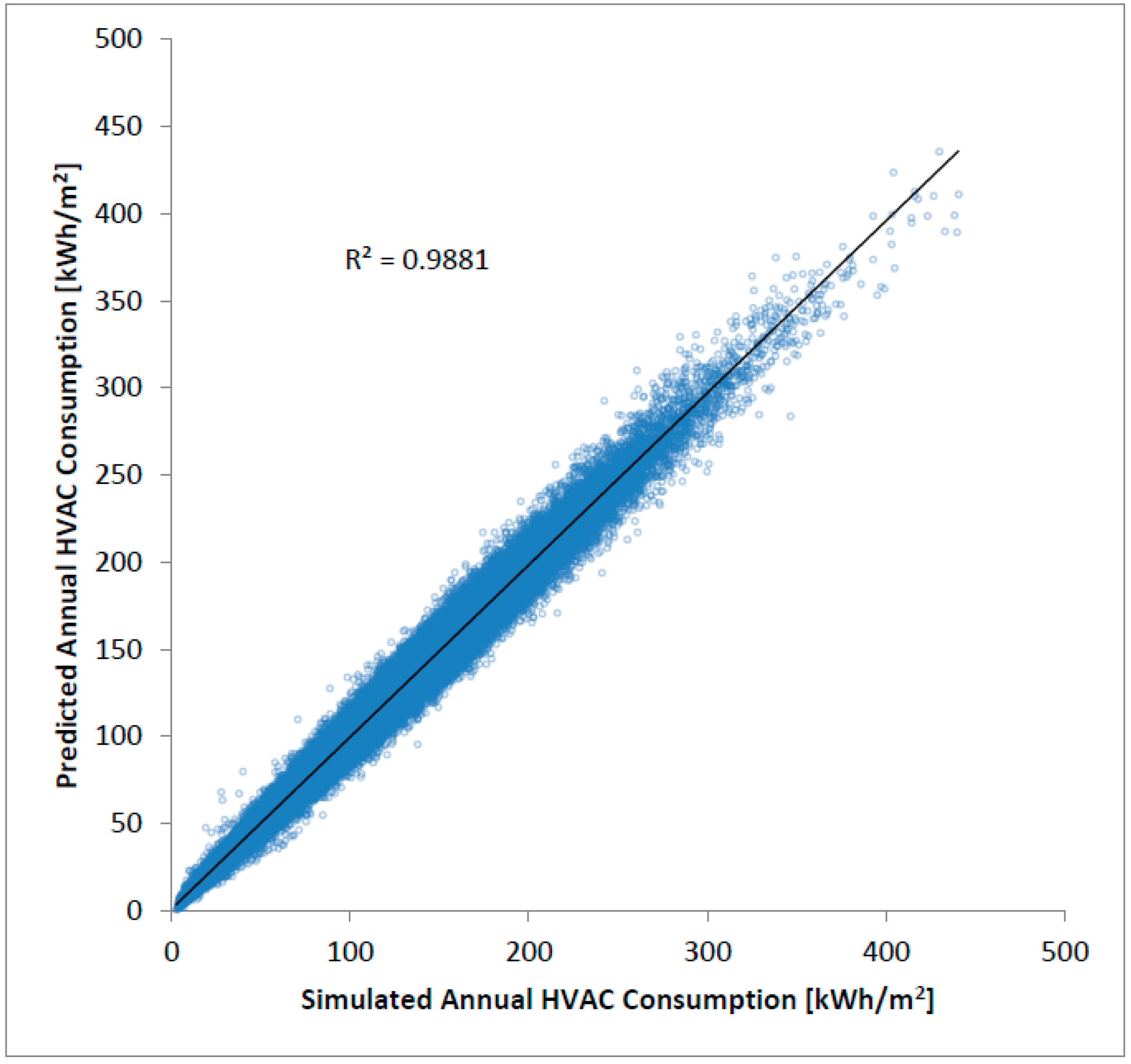
The neural network with 32 neurons in the hidden layer presented better performance (higher SI value) and, therefore, it was used as the baseline in the following studies. This network was called ANN32. Figure 7 shows the results obtained when this ANN was used to predict the annual HVAC energy consumption of all cases.

After establishing the number of neurons in the hidden layer, the influence of the inclusion, exclusion, or alteration of predictor variables was evaluated. The first change analyzed was the inclusion of a new predictor variable, the number of daily hours of operation of the HVAC system. A new ANN was trained (using cross-validation with 10 k-fold repeated six times) including this predictor variable and keeping 32 neurons in the hidden layer, resulting in values of R² = 0.9885, RMSE = 5.20669, and NRMSE = 0.061313. Therefore, the improvement in the performance measures was small when compared to the baseline (reduction of 1.7% in the RMSE), and it did not justify the increase in the complexity of the metamodel.

Another change analyzed was the substitution of the IPLV value as predictor variable by the values of COP at 25%, 50%, and 75% chiller capacity, which composes the IPLV calculation. As there was an increase in the number of input neurons (20 instead of 18 in the baseline), new ANNs were created with 32, 35, and 38 neurons in the hidden layer. The best performance was obtained with the network with 35 neurons, where R² = 0.9887, RMSE = 5.158972, and NRMSE = 0.060751. This network was called ANN35_COP. The improvement in the performance measures was slightly better than the previous analysis (reduction of 2.6% in the RMSE when compared to the baseline).

The last modification carried out had the objective of evaluating the influence of the use of the frequency histogram of the cooling demand as predictor variables. The baseline ANN used four values (bins) representing the demand histogram as predictor variables. A new ANN was trained without the use of these values. As there was a decrease in the number of input neurons (14 instead of 18 in the baseline), new ANNs were created with 27, 29, and 32 neurons in the hidden layer. The best performance was obtained with the network with 29 neurons, where R² = 0.9858, RMSE = 5.771209, and NRMSE = 0.067961. This network was called ANN29_wDEM. There was an expected reduction in the performance, but it was not significant enough to discourage the adoption of this architecture for the metamodel.

The performance of the ANN baseline and the new ANNs obtained in the last two studies was also evaluated for new cases. These cases were created using values different from those used when the data was obtained. This procedure is described below.

4.4. Evaluation of Models with Unseen Cases

New cases were modeled and preprocessed in the same way described in Section 3.2 and Section 4.1.

Table 11. Variables and range of values used in the construction of the unseen cases.

Variable	Values
Width of base of building	20 or 40 m
Ratio between length and width	1.75 or 4.75
Number of floors	40
Solar orientation of the building	22.5 or 112.5°
WWR	0.25 or 0.65
Solar factor of glasses	0.27 or 0.57
Thermal transmittance of glasses	4.3 W/m2·K
Solar absorptance of external walls	0.4
Thermal transmittance of external walls	2.6 W/m2·K
Thermal capacity of external walls	145 kJ/m2·K
Solar absorptance of roof	0.5
Thermal transmittance of roof	1.93 W/m2·K
Thermal capacity of roof	106 kJ/m2·K
Thermal capacity of internal walls	145 kJ/m2·K
Air infiltration	0.37 air change per hour
Lighting power density	8.75 or 13.75 W/m2
Occupancy rate	5 or 13 m2/person
Daily working hours of weekdays	9 or 13 h
Weather	6 different weather files
Setpoint	23 °C
Economizer/Heat recovery	Differential Enthalpy/None, or None/Enthalpy, or None/None
Night cycle	Off
Chilled water temperature reset	Off
Ventilation type	Constant Volume or Variable Volume
Supply fan delta pressure	200 or 600 Pa
Chilled water pump configuration	Constant Primary/Variable Secondary, or Constant Primary/No Secondary or Variable Primary/No Secondary
Chilled water pump rated head	30 or 60 × 104 Pa
Condenser water pump rated head	15 or 45 × 104 Pa
Outdoor air flow rate	Level 2
Chiller	7 different chillers (Appendix D)
Number of chillers in parallel	1, 2, 3 or 4

presents the values used to obtain the so-called unseen cases. The number of cases determined by the possible combinations of the values presented in Table 6 amounts to 6,193,152 cases. The sample size of 66,300 cases was determined for estimating a population mean [35] (considering large population) with the confidence level of 99% and desired margin of error equal to 1.0% of the standard deviation of the annual HVAC consumption (standard deviation obtained in the 243,963 simulated cases for the data was 48.47 kWh/m²). The method of sampling was the Latin hypercube.

The ANN32, ANN35_COP, and ANN29_wDEM obtained in the previous step were used to predict the annual HVAC consumption of these unseen cases.

Table 12. Performance measures of ANNs to predict the annual HVAC consumption of the unseen cases.

Neural Network	R2	RMSE	NRMSE
ANN32	0.9730	4.471439	0.072966
ANN35_COP	0.9776	4.108731	0.067047
ANN29_wDEM	0.9789	3.908977	0.063788

shows the performance measures obtained with each ANN when used in this prediction.

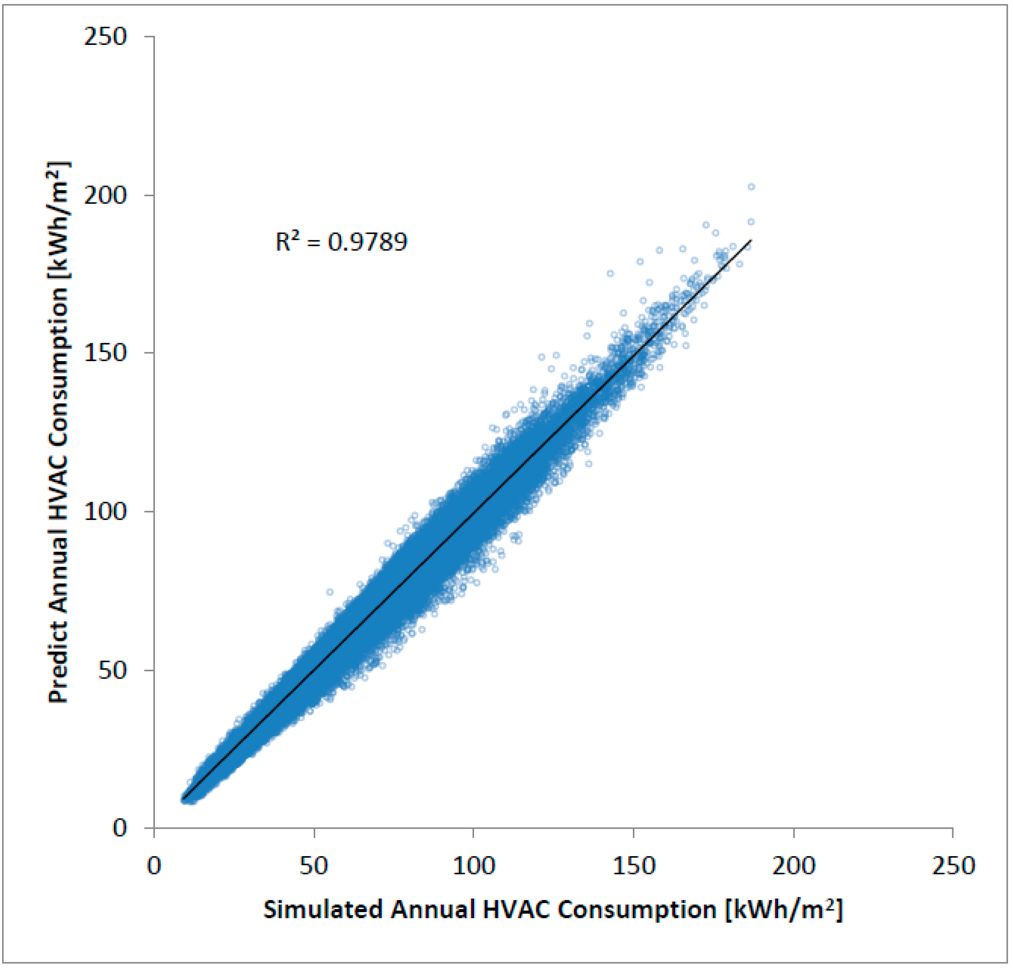
The simpler network (ANN29_wDEM) presented the best performance in the prediction of unseen cases. For this reason, it was considered the final metamodel of this research, which allows us to predict the consumption of Brazilian office buildings from the knowledge of 14 variables (ventilation type, supply fan delta pressure, use of economizer, use of heat recovery, level of outdoor air flow rate, chilled water pump rated head, condenser water pump rated head, use of secondary circuit in chilled water, use of variable chilled water flow, chiller COP at 100% capacity, chiller IPLV, number of chillers in parallel, annual cooling demand per square meter of floor area, and CEH climate indicator). Figure 8 shows the results obtained when the ANN29_wDEM was used to predict the annual HVAC energy consumption of the unseen cases.

5. Discussion

The high values obtained for the coefficient of determination (R² above 0.9) show that there is a strong correlation between the annual building cooling demand and the temperature-based climate indicator (CDH), as well as for the new indicator proposed in this paper (CEH). The CEH presented a better adjustment quality when a linear regression was used to relate annual cooling demand with climate indicator. The standard error reduced about 20% (from 12.11 to 9.50 kWh/m²·year) when CEH was used in place of the usual CDH. The variation in the base enthalpy and base temperature values allows us to conclude that these values do not significantly influence if the values used are close to 37 kJ/kg and 18 °C respectively.

The building cooling demand cannot be predicted simply from the calculation of the climate indicator (CEH) of the city where it is built. This demand will be the result of several factors that characterize the building, such as construction materials, usage patterns, equipment density, lighting power density, and occupation, among others. The climate indicator is often used as the dependent variable in prediction energy models to determine reference values (benchmark), and its main function is to adjust the consumption value for the climate under analysis.

Regression analysis is one of the most popular techniques for the development of models for building energy consumption prediction [42]. When the regression equations are obtained from a complete and accurate set of experimental data, they can provide precise results in an easier and faster way than using building simulation tools [43]. Artificial intelligence methods, especially artificial neural networks, have recently been used in models for building energy consumption predictions. In both methods, it is necessary to characterize the climate with the smallest possible number of variables in order to simplify the model. Therefore, the results obtained in this research demonstrate that the CEH indicator can be used for this purpose.

The results obtained for the 407 Brazilian cities confirmed the good performance of the CEH with climate indicator, since the R² value remained high (0.9533) and the standard error low (11.00 kWh/m²·year). They also showed the CEH performed better than the CDH_H indicator based on the proposal of Shin and Do [20] whose results were R² = 0.9418 and standard error = 12.27 kWh/m²·year. The representation of the Brazilian climate in the 18 suggested climate zones was adequate due to the observed frequency distribution (Figure 6).

The CDH, CDH_H, and CEH indicators were also evaluated for buildings other than the building model, and again the results showed that the CEH had the best performance. Therefore, the energy consumption prediction model proposed here could be developed for Brazilian office buildings considering the CEH indicator and these eighteen climate zones.

The sensitivity analysis indicated that the annual cooling demand and annual HVAC energy consumption were less sensitive to the changes in the thermal characteristics of the walls and roof (solar absorptance, thermal transmittance, and thermal capacity), in agreement with the results obtained by Lam et al. [44,45]. The annual HVAC energy consumption also was less sensitive to the use of night cycle and chilled water temperature reset.

The use of all simulated cases (243,963) in the ANN training process is impracticable and so it was necessary to define the ideal size for training. ANNs obtained with larger samples present better performance, but they require longer processing time in their training process. The results showed that for this population the use of samples with 36,594 cases generated ANNs with compatible performance to those generated with larger samples. This sample size corresponds to the value determined for estimating a population mean with the confidence levels equal to 95% and desired margin of error equal to 1% of the standard deviation of the variable of interest. In this case, the size calculated as described above represented 15% of the population, but this percentage may not be generalized to other cases. In each new situation the sample size must be calculated using the estimation of population mean technique.

The increase in the size of the hidden layer of the neural network had a greater influence on its performance than the increase in the sample size, in the same way that was observed by Versage [46]. The use of the synthesis index allowed us to define the ideal number of neurons as 32 in the hidden layer of the ANN with 18 neurons in the input layer and 1 neuron in the output layer (initially idealized architecture).

Neural network improvement studies showed that the inclusion of a new variable (daily hours of HVAC system operation) generated a small increase in the network performance (reduction of 1.7% in the RMSE) and did not justify the adoption of this change. These studies indicated that two other alterations could be justifiable: Replacing the IPLV input variable by COP at 25%, at 50%, and at 75% chiller capacity; and excluding the four input variables that characterize the frequency histogram of the cooling demand. Then, these two new ANNs and the baseline ANN were used to predict the annual HVAC system consumption of 66,300 new cases, which were generated with values not used when creating the data; the results demonstrated that the performance of these three ANNs are similar. Thus, the ANN with less complex architecture was adopted as the final metamodel of this research.

6. Conclusions

Climate indicators that only use the dry bulb temperature in their calculations (CDD and CDH) do not consider the presence of the latent heat fraction present in the building cooling demand. This limitation has an influence on the models of building energy prediction that use these indicators in hot and humid climates, because the energy spent in these climates is significant for the air dehumidification process.

The CEH indicator proposed in this paper was more accurate and it could be used as a climate indicator in models of cooling demand prediction for the Brazilian climate. After performing an analysis to determine which values of base temperature and base enthalpy should be employed, we conclude that the most appropriate values are 18 °C and 35 kJ/kg, respectively. A small variation around these values did not present a significant change in the results.

As the CEH calculation is a summation of enthalpy differences of a weather file, similar values of CEH can be obtained from climates with different enthalpy frequency distributions. Even so, the results showed that the CEH indicator is effective in relating the climate to the annual cooling demand. Future work may investigate ways to characterize the difference between these climates that have similar CEH values.

The sensitivity analysis by the Sobol method allowed the reduction of 30% in the number of input variables previously idealized in the process of creating the cases that composed the data of this research. The changes in the thermal characteristics of the walls and roof (solar absorptance, thermal transmittance and thermal capacity) have less influence on cooling demand and HVAC consumption than changes in the other characteristics of the building.

Artificial neural networks of good performance can be trained with a sample whose size is calculated estimating a population mean with the confidence levels equal to 95% and desired margin of error equal to 1% of the standard deviation of the variable of interest.

The metamodel with 14 neurons in the input layer (variables 1 to 14 in Table 8), 29 neurons in the hidden layer, and 1 neuron in the outer layer presented good performance to predict the annual HVAC consumption for the cases used to obtain the model (R² = 0.9858 and NRMSE = 0.067961), and also for the unseen cases (R² = 0.9789 and NRMSE = 0.063788). This metamodel presented similar performance to the other metamodels analyzed, but it features a less complex architecture.

This research has limitations related to the standard configurations of the statistical package used (nnet package in R), such as the activation function and the optimizer. An advanced configuration could improve on the training time and accuracy of ANNs. The trained neural networks have only one hidden layer, the variation of this hyperparameter could also impact the performance of the model. The metamodel was developed for chilled water HVAC systems; hence it does not apply to other types of HVAC systems (direct expansion, variable refrigerant flow). The occupancy variation and the supposed influence of occupant behavior were not considered, thus characterizing another limitation. Future research can be developed to cover other types of HVAC systems. The results obtained using the metamodel developed here can be compared with results of other simplified HVAC consumption prediction models.