The Influence of the Built Environment on School Children’s Metro Ridership: An Exploration Using Geographically Weighted Poisson Regression Models


Abstract
:1. Introduction
2. Literature Review
2.1. Influence of the Built Environment on Metro Ridership
2.2. Application of GWR in the Transportation Field
3. Study Context and Data
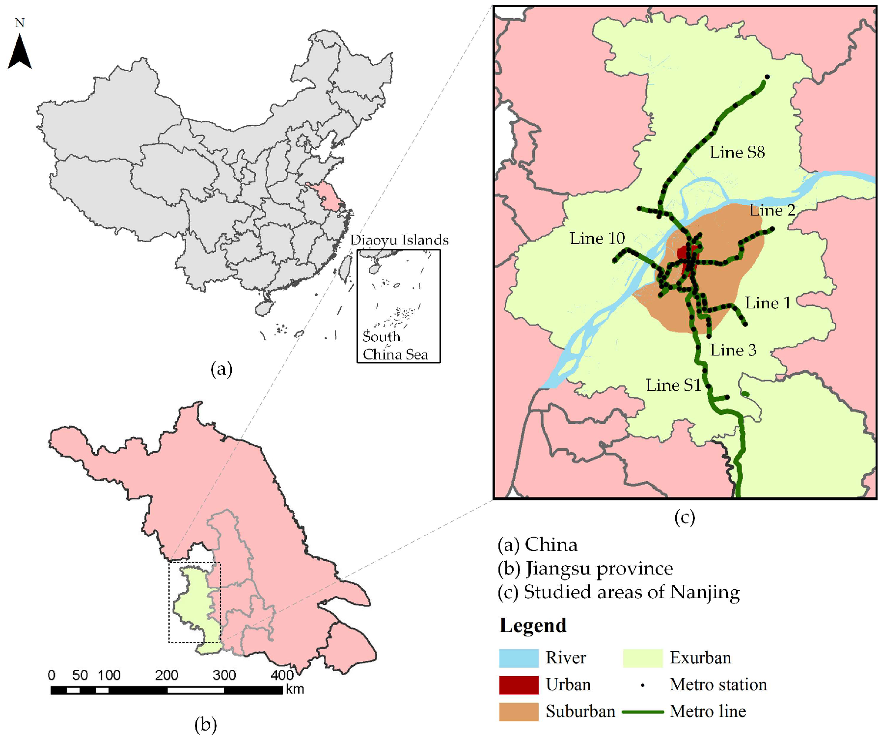
3.1. Study Area Context
3.2. Data Source
3.2.1. Nanjing Metro Smart Card Data
3.2.2. Nanjing Point of Interest (POI) Data
4. Methods
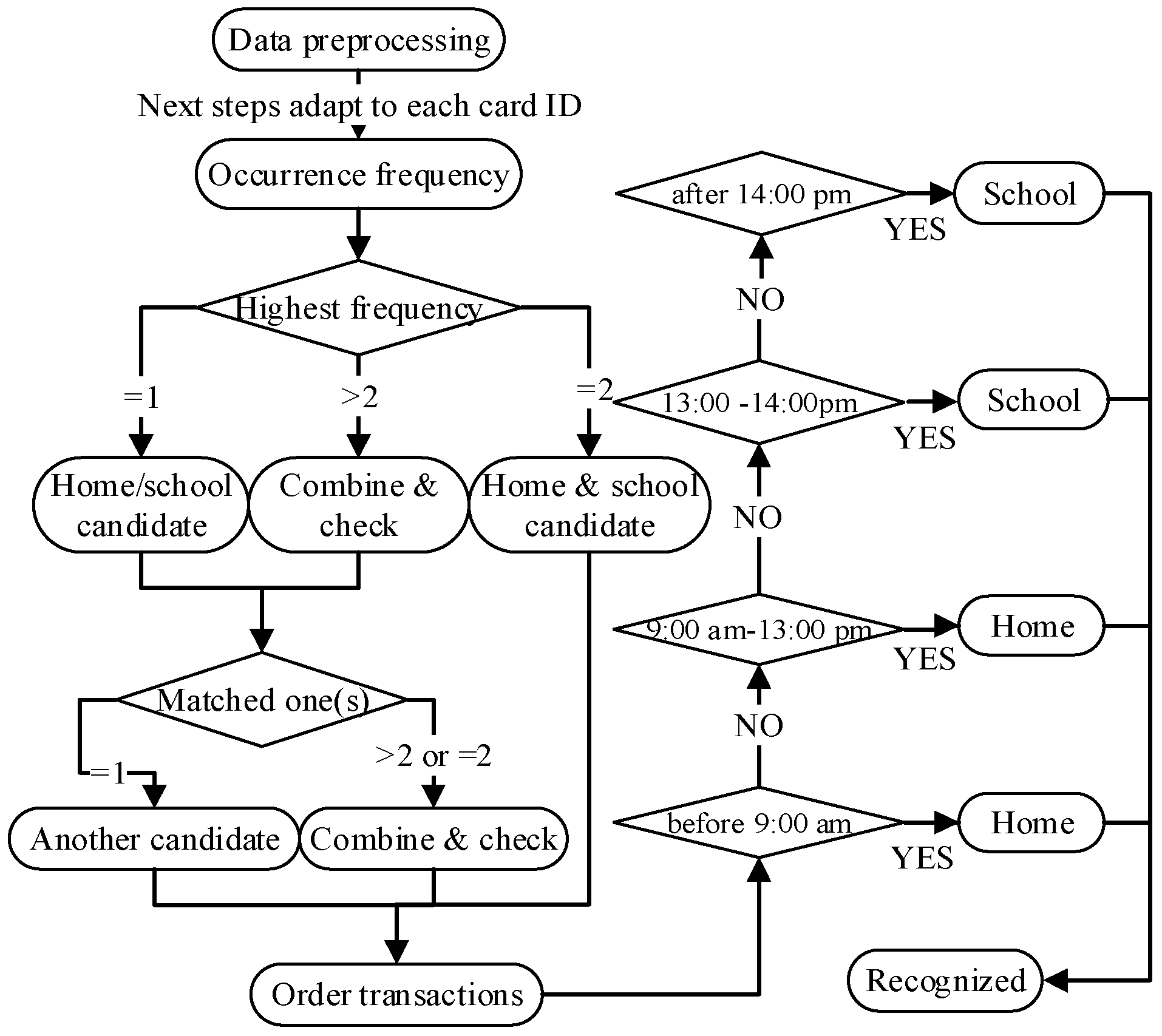
4.1. Identifying School Commuters
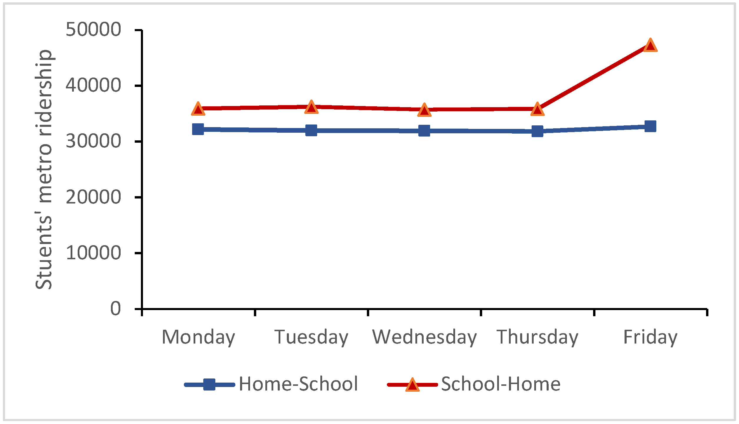
4.2. Calculating the Dependent Variables
4.3. Selecting the Explanatory Variables
4.4. Modeling GWPR
5. Results
5.1. Global Results
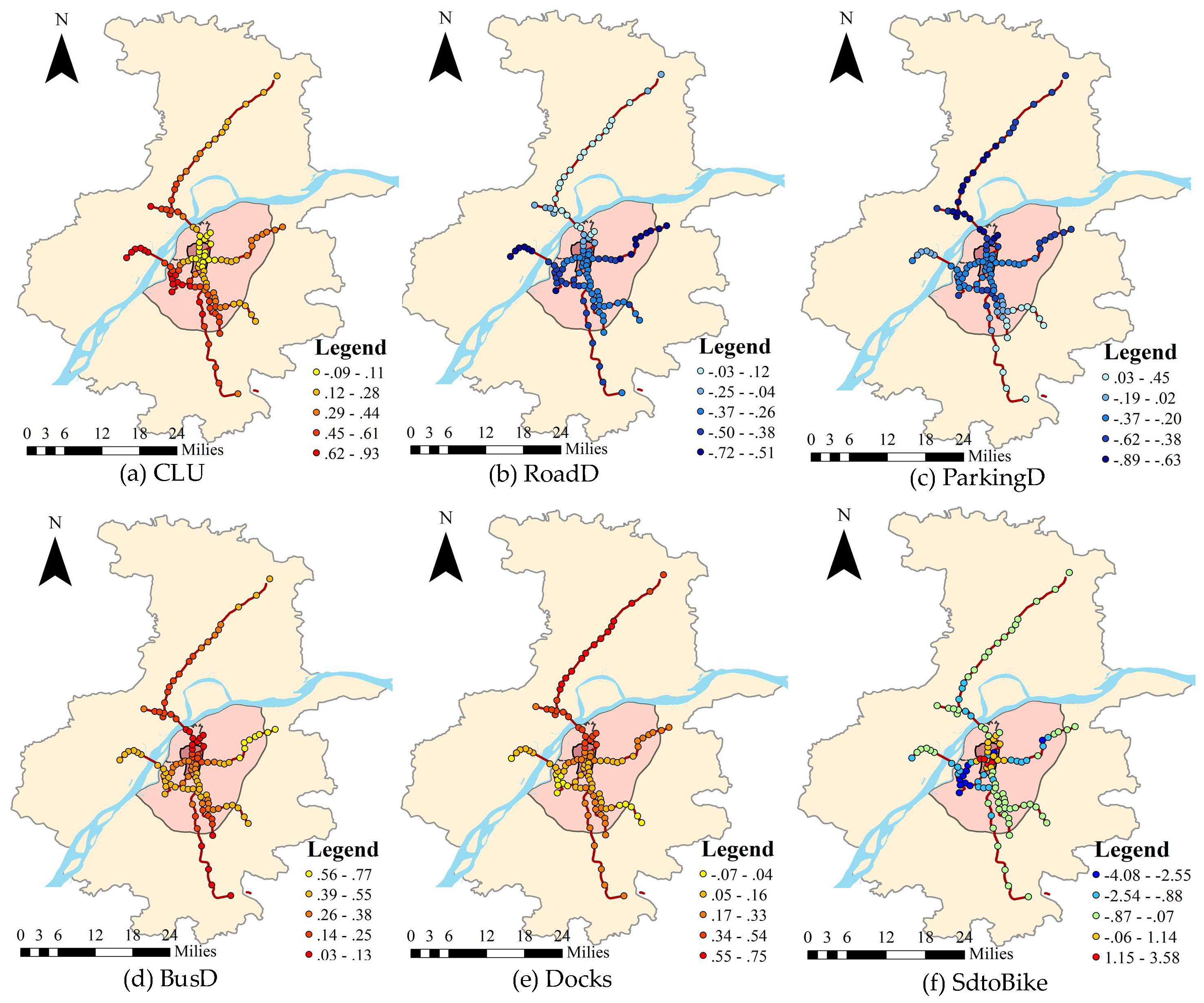
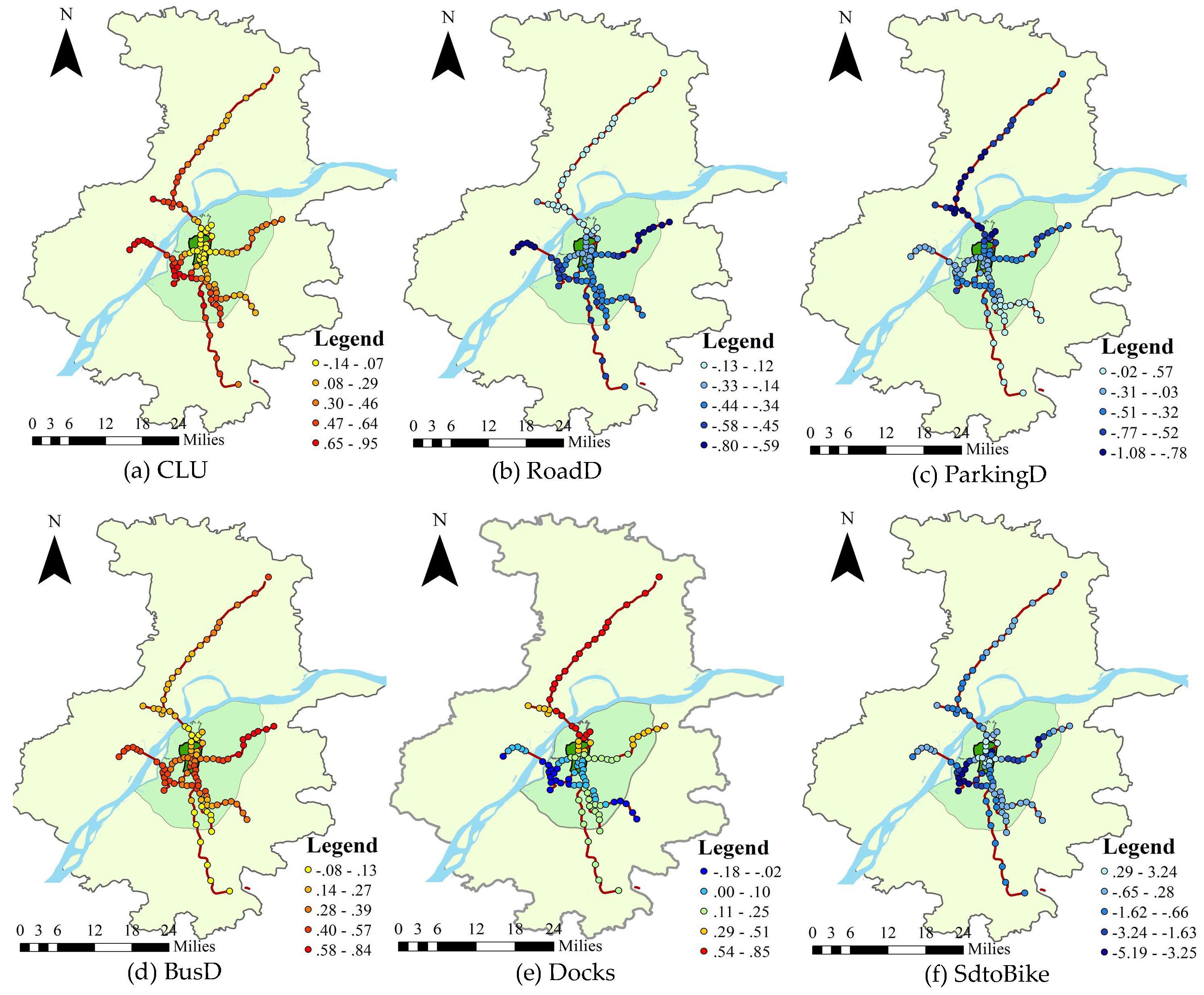
5.2. Local Results
5.3. Analysis and Discussion
6. Implications and Limitations
6.1. Research Implications
6.2. Research Limitations
7. Conclusions
Author Contributions
Funding
Conflicts of Interest
References
- Lu, M.; Sun, C.; Zheng, S. Congestion and pollution consequences of driving-to-school trips: A case study in Beijing. Transp. Res. Part D 2017, 50, 280–291. [Google Scholar] [CrossRef]
- Li, S.; Zhao, P. The determinants of commuting mode choice among school children in Beijing. J. Transp. Geogr. 2015, 46, 112–121. [Google Scholar] [CrossRef]
- Mitra, R. Independent Mobility and Mode Choice for School Transportation: A Review and Framework for Future Research. Transp. Rev. 2013, 33, 21–43. [Google Scholar] [CrossRef]
- He, B.-J.; Zhao, D.-X.; Zhu, J.; Darko, A.; Gou, Z.-H. Promoting and implementing urban sustainability in China: An integration of sustainable initiatives at different urban scales. Habitat Int. 2018, 82, 83–93. [Google Scholar] [CrossRef]
- Mcdonald, N.C. Children’s mode choice for the school trip: The role of distance and school location in walking to school. Transportation 2008, 35, 23–35. [Google Scholar] [CrossRef]
- Sidharthan, R.; Bhat, C.R.; Pendyala, R.M.; Goulias, K.G. Model for Children’s School Travel Mode Choice. Transp. Res. Rec. J. Transp. Res. Board 2011, 2213, 78–86. [Google Scholar] [CrossRef]
- Ermagun, A.; Samimi, A. Promoting active transportation modes in school trips. Transp. Policy 2015, 37, 203–211. [Google Scholar] [CrossRef]
- Sener, I.N.; Lee, R.J.; Sidharthan, R. An examination of children’s school travel: A focus on active travel and parental effects. Transp. Res. Part A Policy Pract. 2018. [Google Scholar] [CrossRef]
- Zhang, R.; Yao, E.; Liu, Z. School travel mode choice in Beijing, China. J. Transp. Geogr. 2017, 62, 98–110. [Google Scholar] [CrossRef]
- Liu, Y.; Ji, Y.; Shi, Z.; He, B.; Liu, Q. Investigating the effect of the spatial relationship between home, workplace and school on parental chauffeurs’ daily travel mode choice. Transp. Policy 2018, 69, 78–87. [Google Scholar] [CrossRef]
- He, S.Y.; Giuliano, G. School choice: Understanding the trade-off between travel distance and school quality. Transportation 2017. [Google Scholar] [CrossRef]
- Mandic, S.; Sandretto, S.; Bengoechea, E.G.; Hopkins, D.; Moore, A.; Rodda, J.; Wilson, G. Enrolling in the Closest School or Not? Implications of school choice decisions for active transport to school. J. Transp. Health 2017, 5, S16–S17. [Google Scholar] [CrossRef]
- Li, J.; Zhang, K.; Guo, J.; Jiang, K. Reasons Analyzing of School Bus Accidents in China. Procedia Eng. 2012, 45, 841–846. [Google Scholar] [CrossRef]
- Gu, Y.; Liu, Y.; Ji, Y.; Ma, X. School Commuting Pattern in Metro System Across Different Loyalty Groups. In Proceedings of the Transportation Research Board 97th Annual Meeting, Washington, DC, USA, 7–11 January 2018. [Google Scholar]
- Mitra, R.; Buliung, R.N.; Roorda, M.J. Built Environment and School Travel Mode Choice in Toronto, Canada. Transp. Res. Rec. J. Transp. Res. Board 2010, 2156, 10–1443. [Google Scholar] [CrossRef]
- Broberg, A.; Sarjala, S. School travel mode choice and the characteristics of the urban built environment: The case of Helsinki, Finland. Transp. Policy 2015, 37, 1–10. [Google Scholar] [CrossRef]
- Rothman, L.; Buliung, R.; To, T.; Macarthur, C.; Macpherson, A.; Howard, A. Associations between parents’ perception of traffic danger, the built environment and walking to school. J. Transp. Health 2015, 2, 327–335. [Google Scholar] [CrossRef]
- Ikeda, E.; Stewart, T.; Garrett, N.; Egli, V.; Mandic, S.; Hosking, J.; Witten, K.; Hawley, G.; Tautolo, E.S.; Rodda, J. Built environment associates of active school travel in New Zealand children and youth: A systematic meta-analysis using individual participant data. J. Transp. Health 2018, 9, 117–131. [Google Scholar] [CrossRef]
- Zhao, J.; Deng, W.; Song, Y.; Zhu, Y. What influences Metro station ridership in China? Insights from Nanjing. Cities 2013, 35, 114–124. [Google Scholar] [CrossRef]
- Gan, Z.; Yang, M.; Feng, T.; Timmermans, H. Understanding urban mobility patterns from a spatiotemporal perspective: Daily ridership profiles of metro stations. Transportation 2018. [Google Scholar] [CrossRef]
- Singh, N.; Vasudevan, V. Understanding school trip mode choice—The case of Kanpur (India). J. Transp. Geogr. 2018, 66, 283–290. [Google Scholar] [CrossRef]
- Ross, T.; Buliung, R. A systematic review of disability’s treatment in the active school travel and children’s independent mobility literatures. Transp. Rev. 2018, 38, 349–371. [Google Scholar] [CrossRef]
- Huang, X.; Tan, J. Understanding spatio-temporal mobility patterns for seniors, child/student and adult using smart card data. Int. Arch. Photogramm. Remote. Sens. Spat. Inf. Sci. 2014, XL-1, 167–172. [Google Scholar] [CrossRef]
- Gutiérrez, J.; Cardozo, O.D.; García-Palomares, J.C. Transit ridership forecasting at station level: An approach based on distance-decay weighted regression. J. Transp. Geogr. 2011, 19, 1081–1092. [Google Scholar] [CrossRef]
- Kuby, M.; Barranda, A.; Upchurch, C. Factors influencing light-rail station boardings in the United States. Transp. Res. Part A 2004, 38, 223–247. [Google Scholar] [CrossRef]
- Sohn, K.; Shim, H. Factors generating boardings at Metro stations in the Seoul metropolitan area. Cities 2010, 27, 358–368. [Google Scholar] [CrossRef]
- Ji, Y.; Ma, X.; Yang, M.; Jin, Y.; Gao, L. Exploring Spatially Varying Influences on Metro-Bikeshare Transfer: A Geographically Weighted Poisson Regression Approach. Sustainability 2018, 10, 1526. [Google Scholar] [CrossRef]
- Mcmillen, D.P. Geographically Weighted Regression: The Analysis of Spatially Varying Relationships. Am. J. Agric. Econ. 2004, 86, 554–556. [Google Scholar] [CrossRef]
- Huang, B.; Wu, B.; Barry, M. Geographically and temporally weighted regression for modeling spatio-temporal variation in house prices. Int. J. Geogr. Inf. Sci. 2010, 24, 383–401. [Google Scholar] [CrossRef]
- Yang, J.; Bao, Y.; Zhang, Y.; Li, X.; Ge, Q. Impact of Accessibility on Housing Prices in Dalian City of China Based on a Geographically Weighted Regression Model. Chin. Geogr. Sci. 2018, 28, 505–515. [Google Scholar] [CrossRef]
- Huang, Y.; Wang, X.; Patton, D. Examining spatial relationships between crashes and the built environment: A geographically weighted regression approach. J. Transp. Geogr. 2018, 69, 221–233. [Google Scholar] [CrossRef]
- Mitra, R.; Buliung, R.N. The influence of neighborhood environment and household travel interactions on school travel behavior: An exploration using geographically-weighted models. J. Transp. Geogr. 2014, 36, 69–78. [Google Scholar] [CrossRef]
- AsadKhattak, X. Role of travel information in supporting travel decision adaption: Exploring spatial patterns. Transportmetrica 2013, 9, 316–334. [Google Scholar]
- Feuillet, T.; Commenges, H.; Menai, M.; Salze, P.; Perchoux, C.; Reuillon, R.; Kesse-Guyot, E.; Enaux, C.; Nazare, J.A.; Hercberg, S. A massive geographically weighted regression model of walking-environment relationships. J. Transp. Geogr. 2018, 68, 118–129. [Google Scholar] [CrossRef]
- Chow, L.F.; Zhao, F.; Liu, X.; Li, M.T.; Ubaka, I. Transit Ridership Model Based on Geographically Weighted Regression. Transp. Res. Rec. J. Transp. Res. Board 2006, 1972, 105–114. [Google Scholar] [CrossRef]
- Cardozo, O.D.; García-Palomares, J.C.; Gutiérrez, J. Application of geographically weighted regression to the direct forecasting of transit ridership at station-level. Appl. Geogr. 2012, 34, 548–558. [Google Scholar] [CrossRef]
- Chiou, Y.C.; Jou, R.C.; Yang, C.H. Factors affecting public transportation usage rate: Geographically weighted regression. Transp. Res. Part A Policy Pract. 2015, 78, 161–177. [Google Scholar] [CrossRef]
- Tu, W.; Cao, R.; Yue, Y.; Zhou, B.; Li, Q.; Li, Q. Spatial variations in urban public ridership derived from GPS trajectories and smart card data. J. Transp. Geogr. 2018, 69, 45–57. [Google Scholar] [CrossRef]
- Ma, X.; Zhang, J.; Ding, C.; Wang, Y. A geographically and temporally weighted regression model to explore the spatiotemporal influence of built environment on transit ridership. Comput. Environ. Urban Syst. 2018, 70, 113–124. [Google Scholar] [CrossRef]
- Bureau, N.S. Nanjing National Economic and Social Development Statistics Bulletin; Nanjing Statistics Bureau: Nanjing, China, 2015. [Google Scholar]
- Government, T.C. Notice on Adjusting the Standards for Categorizing City Sizes. Available online: http://english.gov.cn/policies/latest_releases/2014/11/25/content_281475015213546.htm. (accessed on 20 November 2014).
- Long, Y.; Thill, J.C. Combining smart card data and household travel survey to analyze jobs–housing relationships in Beijing. Comput. Environ. Urban Syst. 2013, 53, 19–35. [Google Scholar] [CrossRef]
- Le, M.K.; Bhaskar, A.; Chung, E. Passenger Segmentation Using Smart Card Data. IEEE Trans. Intell. Transp. Syst. 2015, 16, 1537–1548. [Google Scholar]
- Medina, S.A.O. Inferring weekly primary activity patterns using public transport smart card data and a household travel survey. Travel Behav. Soc. 2016, 12, 93–101. [Google Scholar] [CrossRef]
- Xia, J.; Nesbitt, J.; Daley, R.; Najnin, A.; Litman, T.; Tiwari, S.P. A multi-dimensional view of transport-related social exclusion: A comparative study of Greater Perth and Sydney. Transp. Res. Part A Policy Pract. 2016, 94, 205–221. [Google Scholar] [CrossRef]
- Nakaya, T.; Fotheringham, A.C.; Charlton, M. Geographically weighted Poisson regression for disease association mapping. Stat. Med. 2010, 24, 2695–2717. [Google Scholar] [CrossRef] [PubMed]
- Wang, Y.; Chau, C.K.; Ng, W.Y.; Leung, T.M. A review on the effects of physical built environment attributes on enhancing walking and cycling activity levels within residential neighborhoods. Cities 2016, 50, 1–15. [Google Scholar] [CrossRef]
- Mcdonald, N.C. Household interactions and children’s school travel: The effect of parental work patterns on walking and biking to school. J. Transp. Geogr. 2008, 16, 324–331. [Google Scholar] [CrossRef]


| Independent Variables | Unit | Max | Min | Mean | S.D. |
|---|---|---|---|---|---|
| Dependent variables | |||||
| Trips to school (TS) | Number | 32,197 | 31,826 | 31,973 | 139.67 |
| Return trips to home (RTH) | Number | 47,324 | 35,726 | 35,933 | 195.47 |
| Land use variables | |||||
| Job density (JobD) | Number/km2 | 431 | 0.00 | 41 | 72.99 |
| Residential-oriented land use (RLU) | Percentage | 1.00 | 0.00 | 0.06 | 0.10 |
| Commercial-oriented land use (CLU) | Percentage | 0.83 | 0.00 | 0.50 | 0.19 |
| Educational-oriented land use (ELU) | Percentage | 0.70 | 0.00 | 0.07 | 0.10 |
| Transferring-related variables | |||||
| Density of P&R (ParkingD) | Number/km2 | 40.78 | 0.00 | 5.33 | 6.82 |
| Density of bus stations (BusD) | Number/km2 | 40.78 | 0.00 | 12.00 | 10.42 |
| Density of bike stations (BikeD) | Number/km2 | 8.95 | 0.00 | 1.83 | 2.37 |
| Docks at bikeshare stations (Docks) | Number/km2 | 389.94 | 0.00 | 69.80 | 92.79 |
| External connectivity variables | |||||
| Density of intersections (IntersectionD) | Number/km2 | 18.54 | 0.56 | 5.71 | 3.86 |
| Density of road networks (RoadD) | km/km2 | 27.78 | 3.98 | 16.04 | 5.34 |
| Shortest distance between bus station and metro station (SDtoBus) | m | 3695.94 | 1.98 | 379.15 | 660.68 |
| Shortest distance between bike station and metro station (SDtoBike) | m | 42,693.46 | 16.21 | 5850.36 | 8792.79 |
| Dependent | Trips to School (TS) | Return Trips to Home (RTH) | ||||
|---|---|---|---|---|---|---|
| Variable | Coef. | S.E. | Z-Stat. | Coef. | S.E. | Z-Stat. |
| Intercept | 5.377 | 0.007 | 746.032 *** | 5.474 | 0.007 | 782.499 *** |
| CLU | 0.446 | 0.007 | 61.512 *** | 0.444 | 0.007 | 63.789 *** |
| RoadD | −0.407 | 0.008 | −50.420 *** | −0.368 | 0.008 | −47.939 *** |
| ParkingD | −0.387 | 0.011 | −36.112 *** | −0.315 | 0.009 | −33.659 *** |
| BusD | 0.404 | 0.008 | 48.358 *** | 0.393 | 0.008 | 50.676 *** |
| Docks | 0.183 | 0.008 | 23.052 *** | 0.183 | 0.007 | 24.677 *** |
| SDtoBike | −0.575 | 0.010 | −56.195 *** | −0.607 | 0.010 | −58.849 *** |
| AIC | 20,495.239 | 19,214.216 | ||||
| AICc | 20,496.305 | 19,215.282 | ||||
| Percent deviance explained | 0.429 | 0.482 | ||||
| Local Terms | Mean | Min | Low Quartile | Median | Upper Quartile | Max | DIFF of Criterion * |
|---|---|---|---|---|---|---|---|
| Intercept | 5.201 | 2.377 | 4.94 | 5.253 | 5.787 | 8.069 | −648.232 |
| CLU | 0.352 | −0.145 | 0.175 | 0.363 | 0.562 | 0.95 | −1888.56 |
| RoadD | −0.336 | −0.798 | −0.493 | −0.397 | −0.176 | 0.12 | −1244.441 |
| ParkingD | −0.352 | −1.078 | −0.548 | −0.349 | −0.228 | 0.569 | −1337.879 |
| BusD | 0.329 | −0.084 | 0.196 | 0.342 | 0.436 | 0.84 | −879.722 |
| Docks | 0.238 | −0.181 | 0.026 | 0.167 | 0.448 | 0.852 | −1055.801 |
| SDtoBike | −0.862 | −5.192 | −1.103 | −0.624 | −0.382 | 3.237 | −519.315 |
| AIC | 10,730.82 | AICc | 10,748.06 | Percent of deviance explained 0.702 | |||
| Local Terms | Mean | Min | Low Quartile | Median | Upper Quartile | Max | DIFF of Criterion * |
|---|---|---|---|---|---|---|---|
| Intercept | 5.456 | 3.143 | 5.188 | 5.395 | 5.890 | 8.451 | −695.618 |
| CLU | 0.360 | −0.090 | 0.192 | 0.337 | 0.546 | 0.928 | −1992.976 |
| RoadD | −0.290 | −0.721 | −0.433 | −0.338 | −0.145 | 0.115 | −1065.073 |
| ParkingD | −0.315 | −0.889 | −0.463 | −0.292 | −0.215 | 0.453 | −1006.787 |
| BusD | 0.328 | 0.026 | 0.198 | 0.329 | 0.430 | 0.772 | −817.654 |
| Docks | 0.246 | −0.065 | 0.090 | 0.191 | 0.396 | 0.745 | −865.232 |
| SDtoBike | −0.634 | −4.076 | −0.961 | −0.626 | −0.273 | 3.582 | −504.021 |
| AIC | 10,724.904 | AICc | 10,741.48 | Percent of deviance explained 0.712 | |||
© 2018 by the authors. Licensee MDPI, Basel, Switzerland. This article is an open access article distributed under the terms and conditions of the Creative Commons Attribution (CC BY) license (http://creativecommons.org/licenses/by/4.0/).
Share and Cite
Liu, Y.; Ji, Y.; Shi, Z.; Gao, L. The Influence of the Built Environment on School Children’s Metro Ridership: An Exploration Using Geographically Weighted Poisson Regression Models. Sustainability 2018, 10, 4684. https://doi.org/10.3390/su10124684
Liu Y, Ji Y, Shi Z, Gao L. The Influence of the Built Environment on School Children’s Metro Ridership: An Exploration Using Geographically Weighted Poisson Regression Models. Sustainability. 2018; 10(12):4684. https://doi.org/10.3390/su10124684
Chicago/Turabian StyleLiu, Yang, Yanjie Ji, Zhuangbin Shi, and Liangpeng Gao. 2018. "The Influence of the Built Environment on School Children’s Metro Ridership: An Exploration Using Geographically Weighted Poisson Regression Models" Sustainability 10, no. 12: 4684. https://doi.org/10.3390/su10124684
APA StyleLiu, Y., Ji, Y., Shi, Z., & Gao, L. (2018). The Influence of the Built Environment on School Children’s Metro Ridership: An Exploration Using Geographically Weighted Poisson Regression Models. Sustainability, 10(12), 4684. https://doi.org/10.3390/su10124684