Land Use and Land Cover Changes, and Environment and Risk Evaluation of Dujiangyan City (SW China) Using Remote Sensing and GIS Techniques


Abstract
1. Introduction
2. Materials and Methods
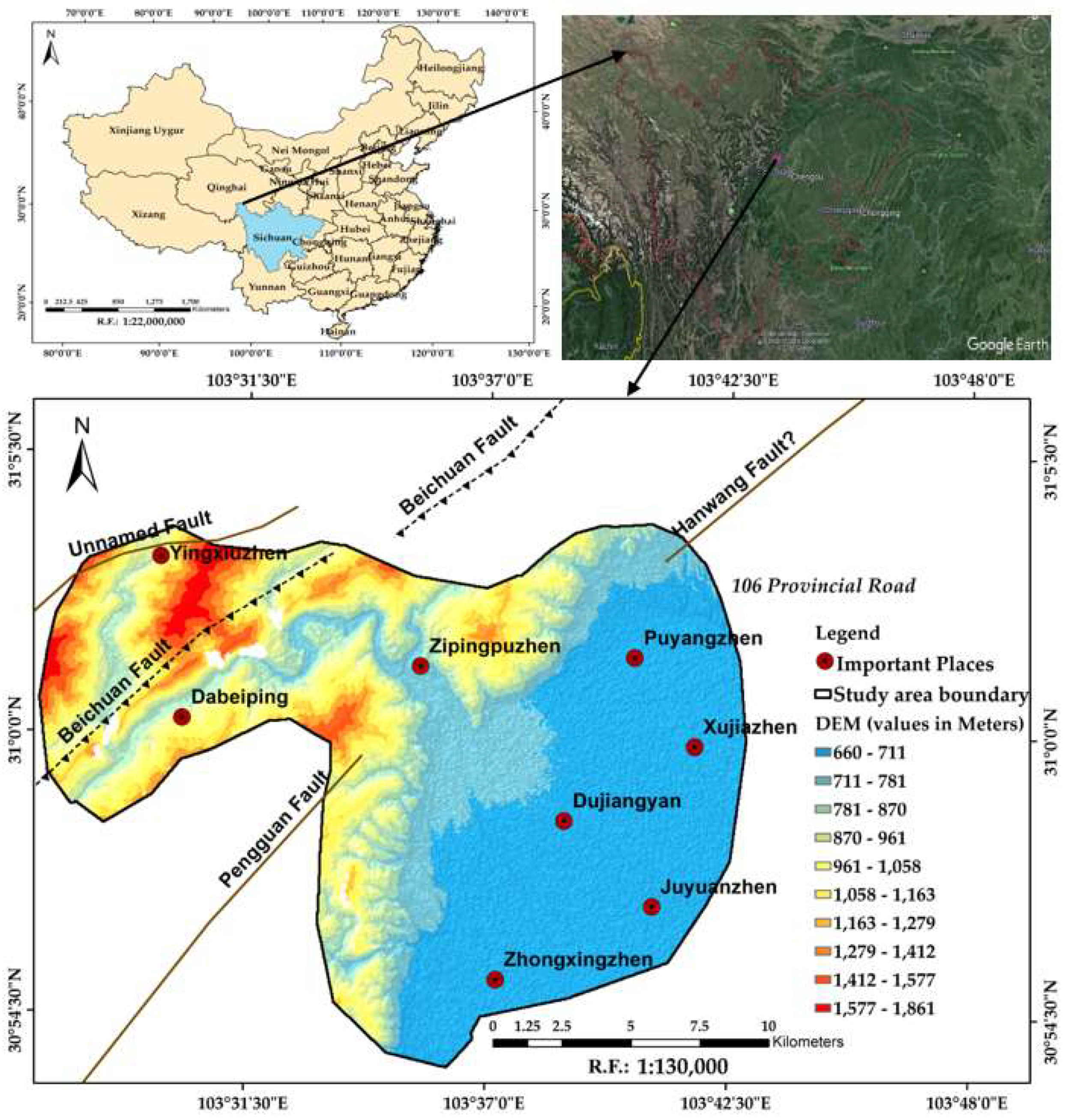
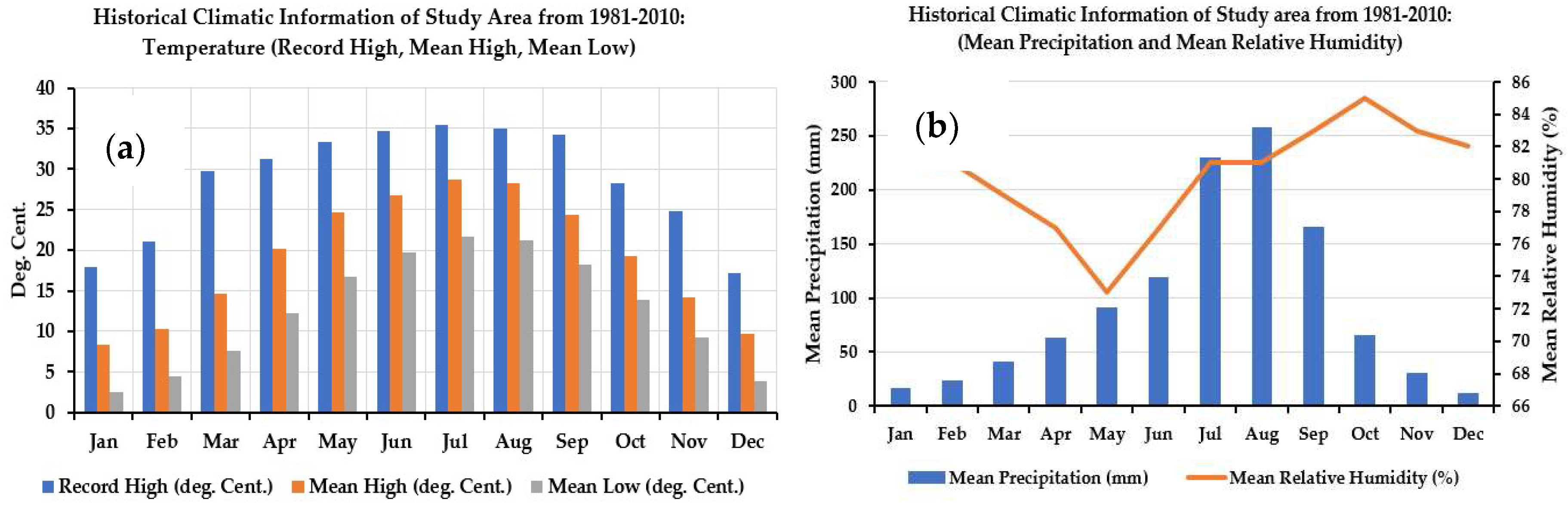
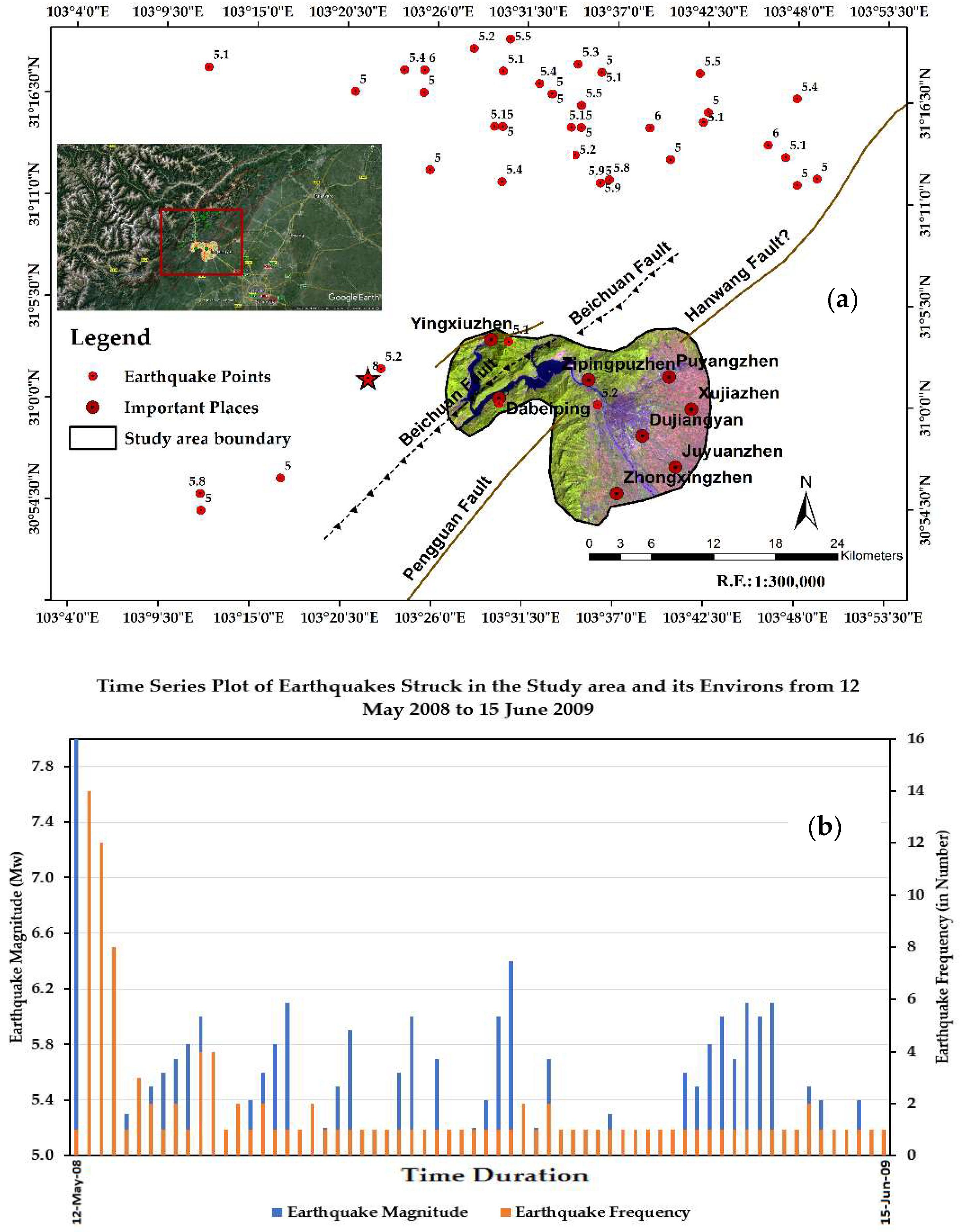
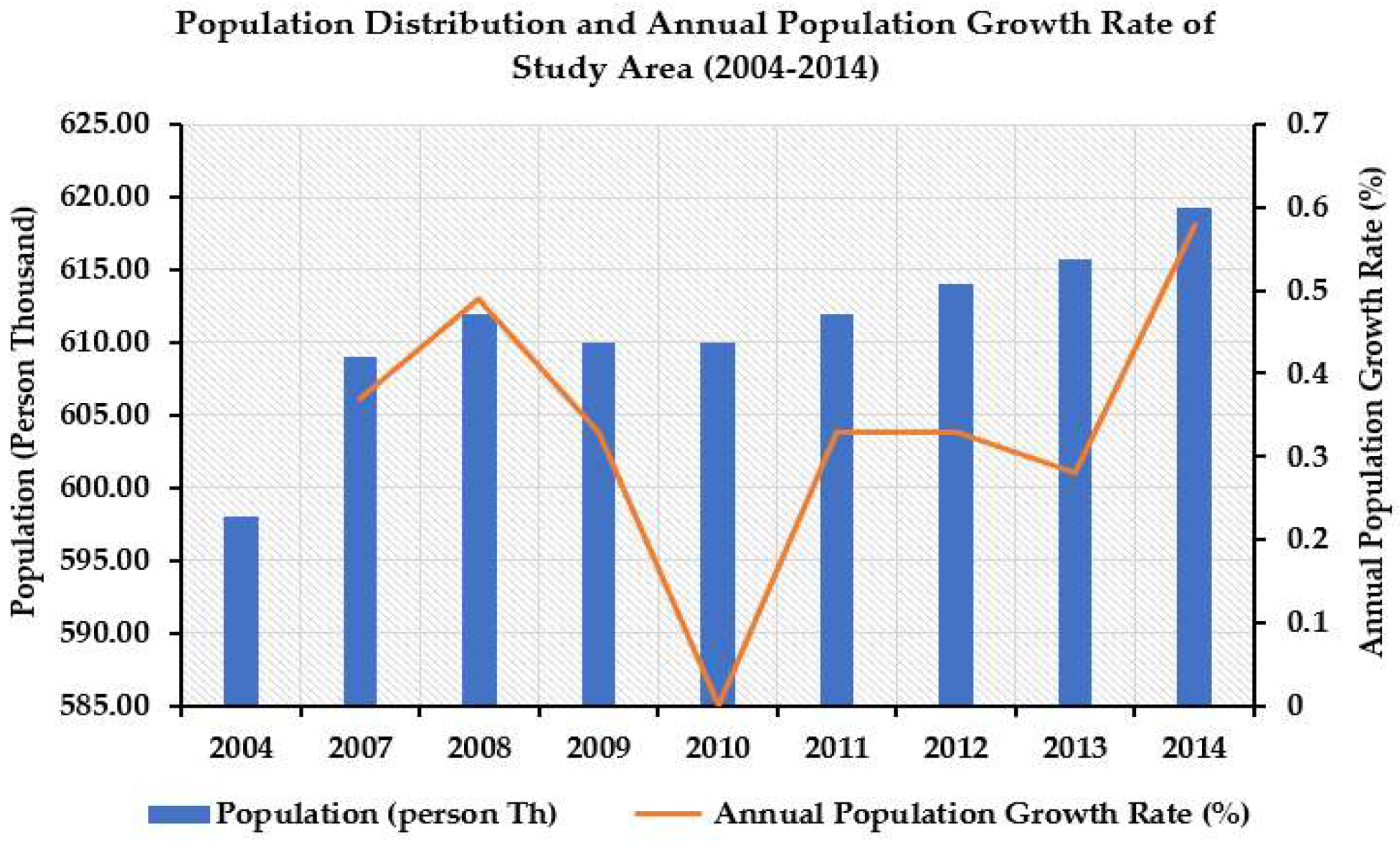
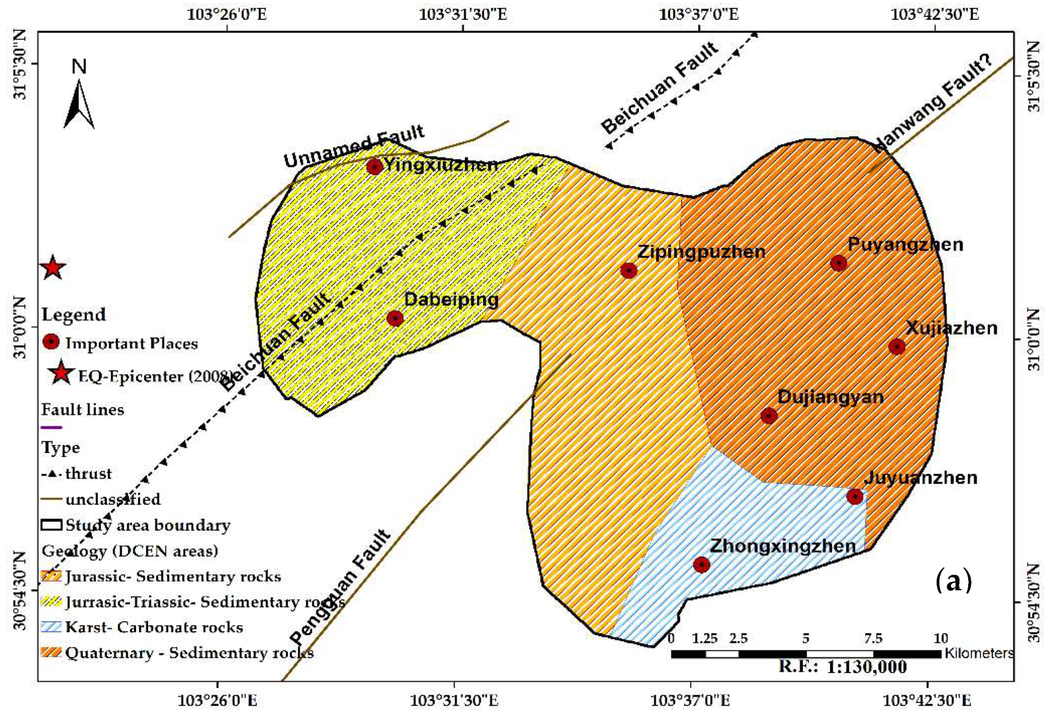
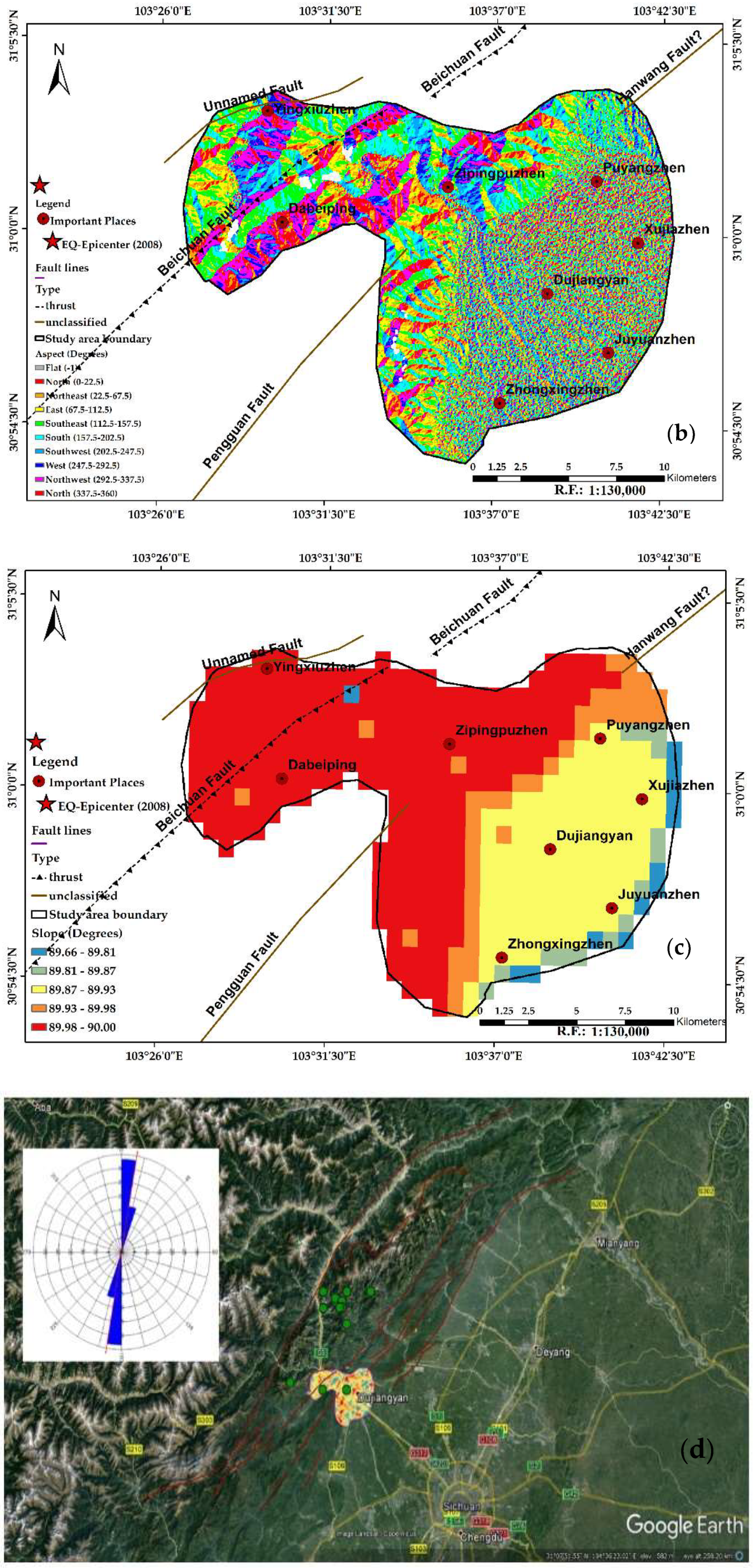
2.1. Study Area
2.2. Data
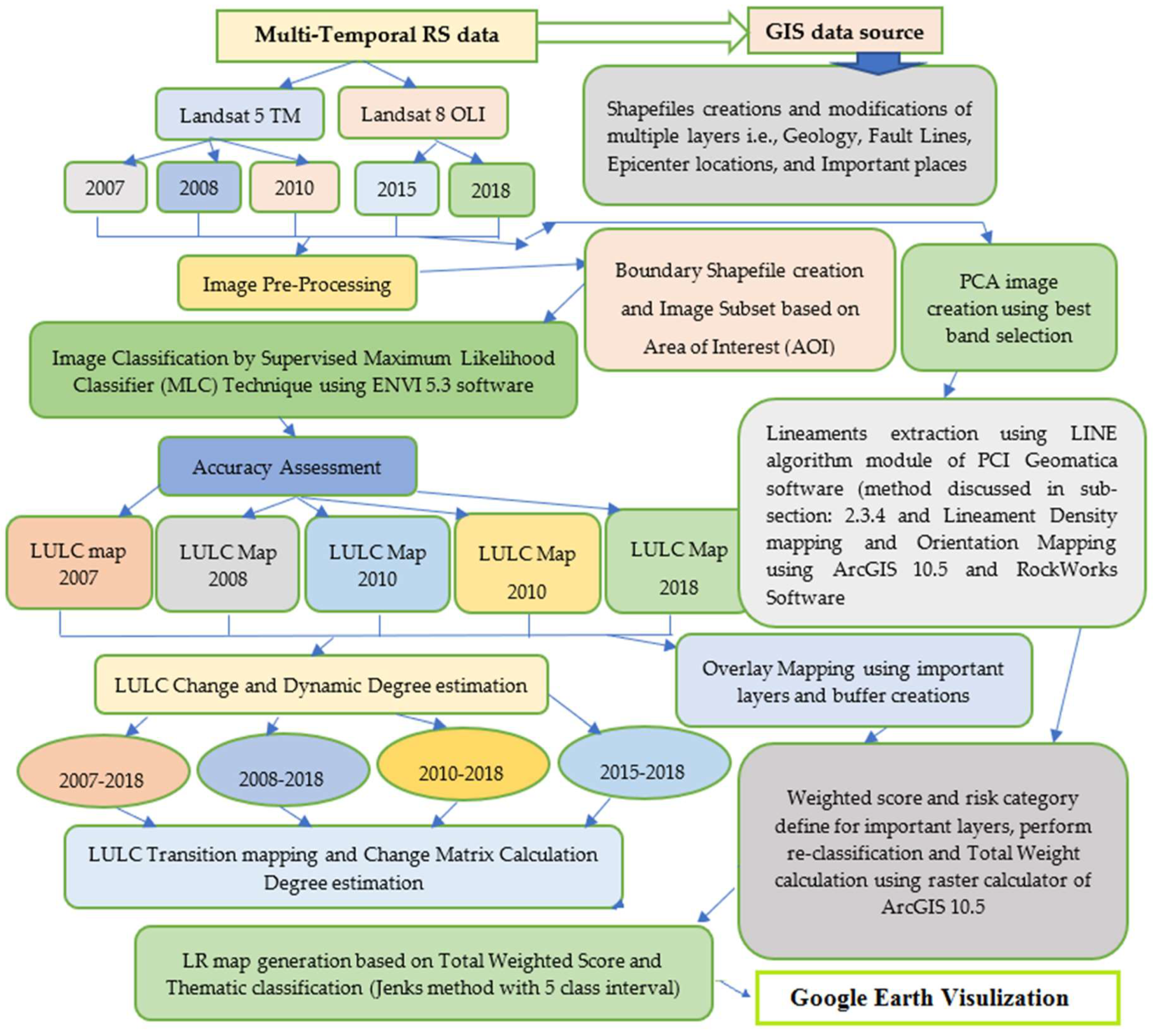
2.3. Methodology
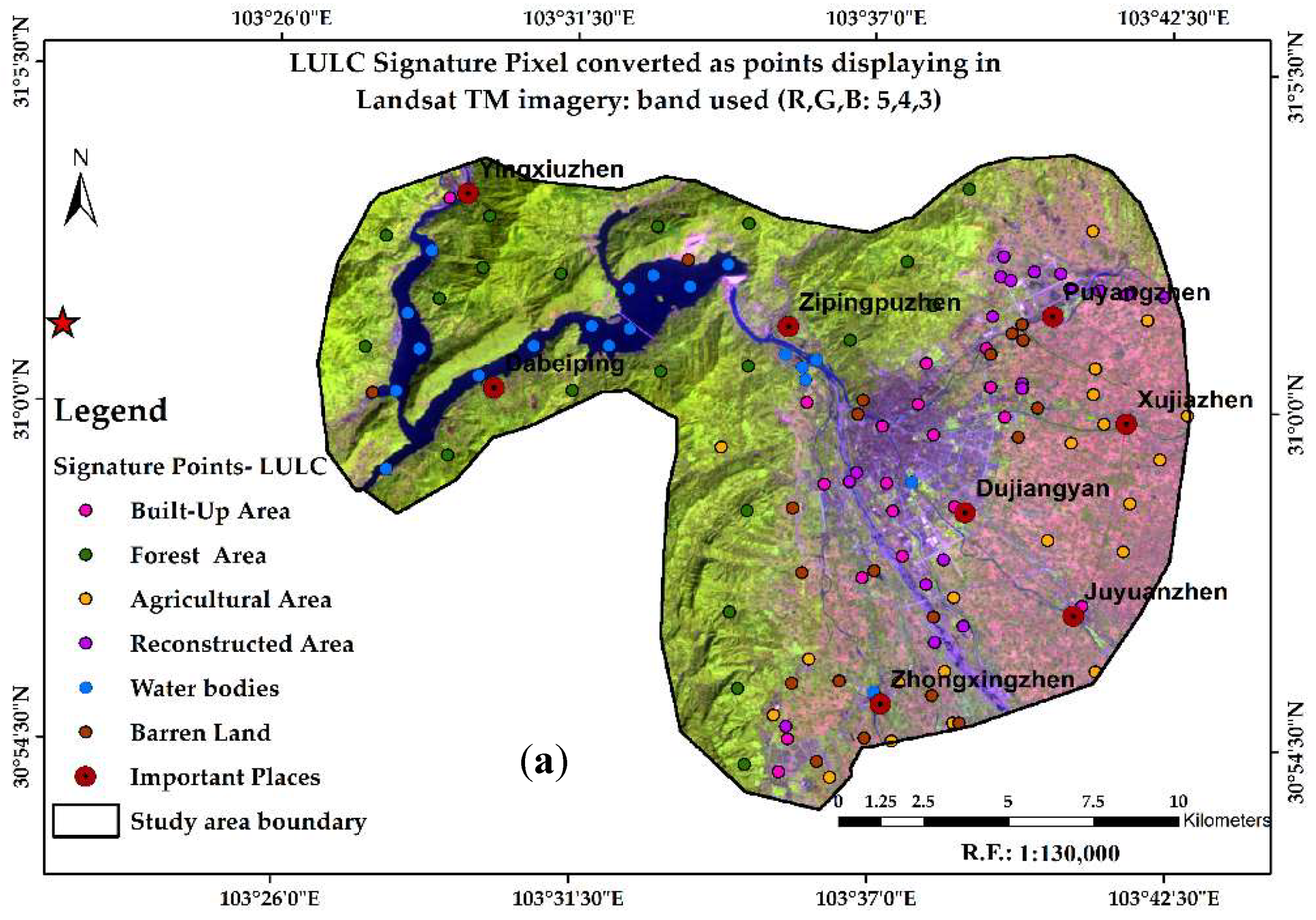
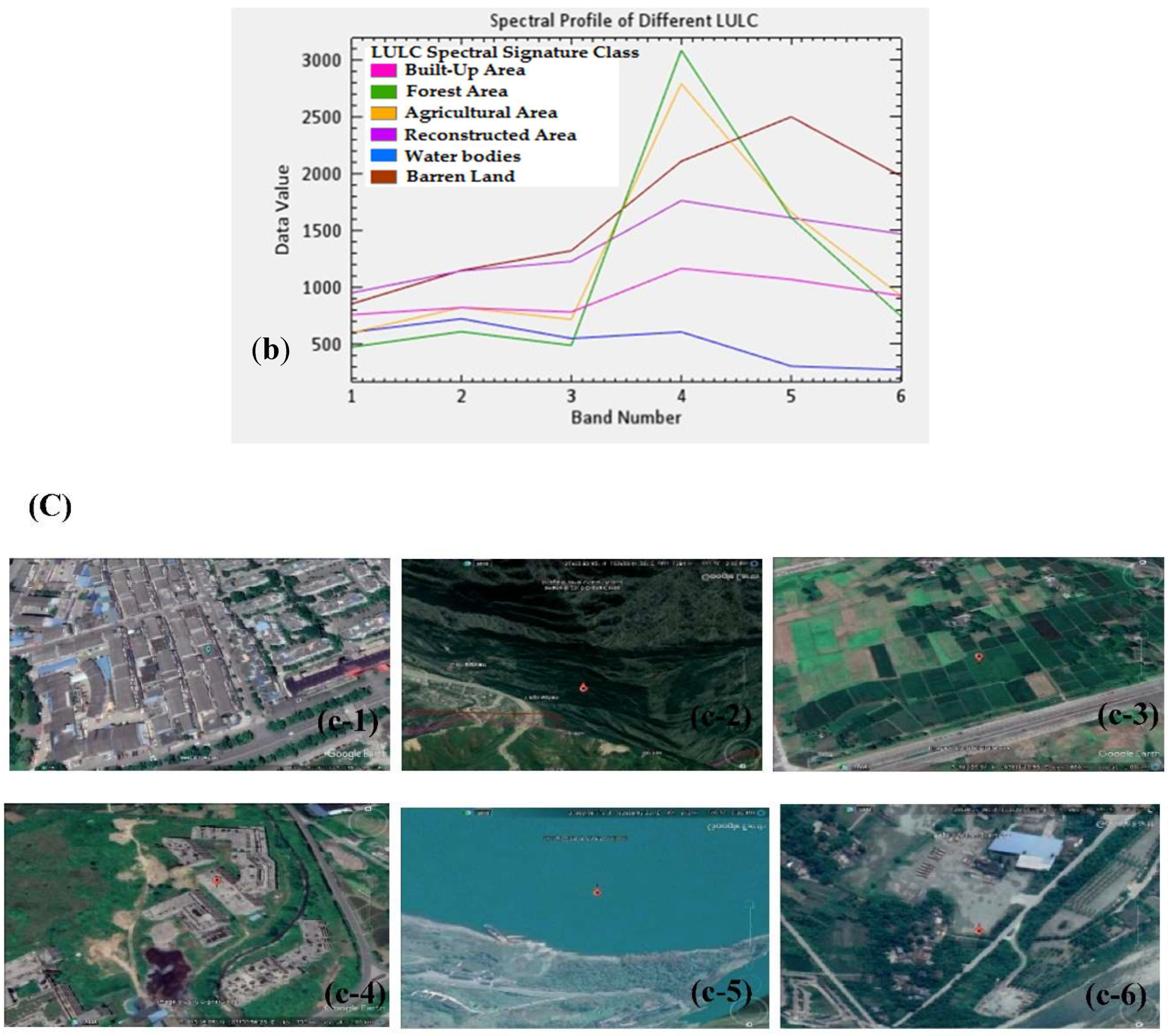
2.3.1. LULC Mapping Training Sample Setup and Classification Accuracy Method
2.3.2. LULC Dynamic Degree Estimation and Transition Matrices Computation Method
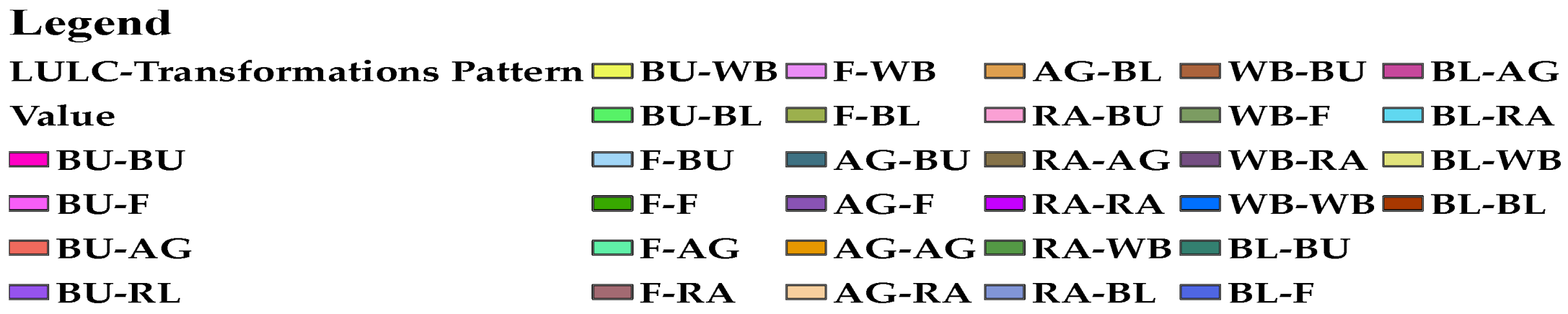
2.3.3. LULC Transitions Mapping and Analysis Method
2.3.4. Landscape Risk Evaluation Method
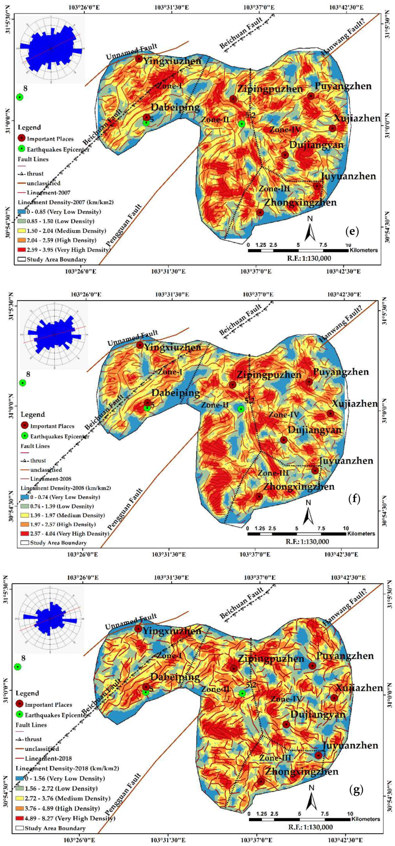
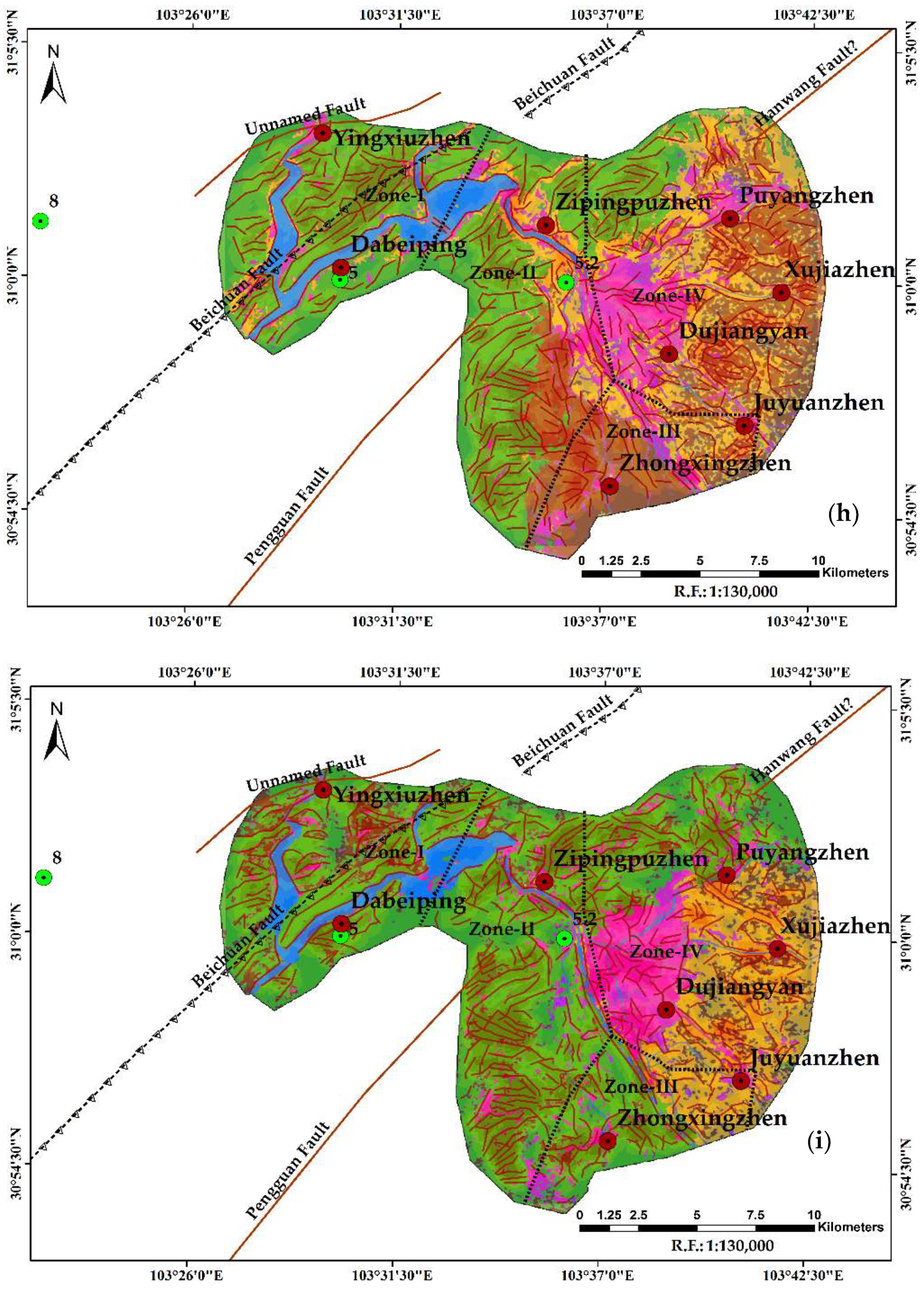
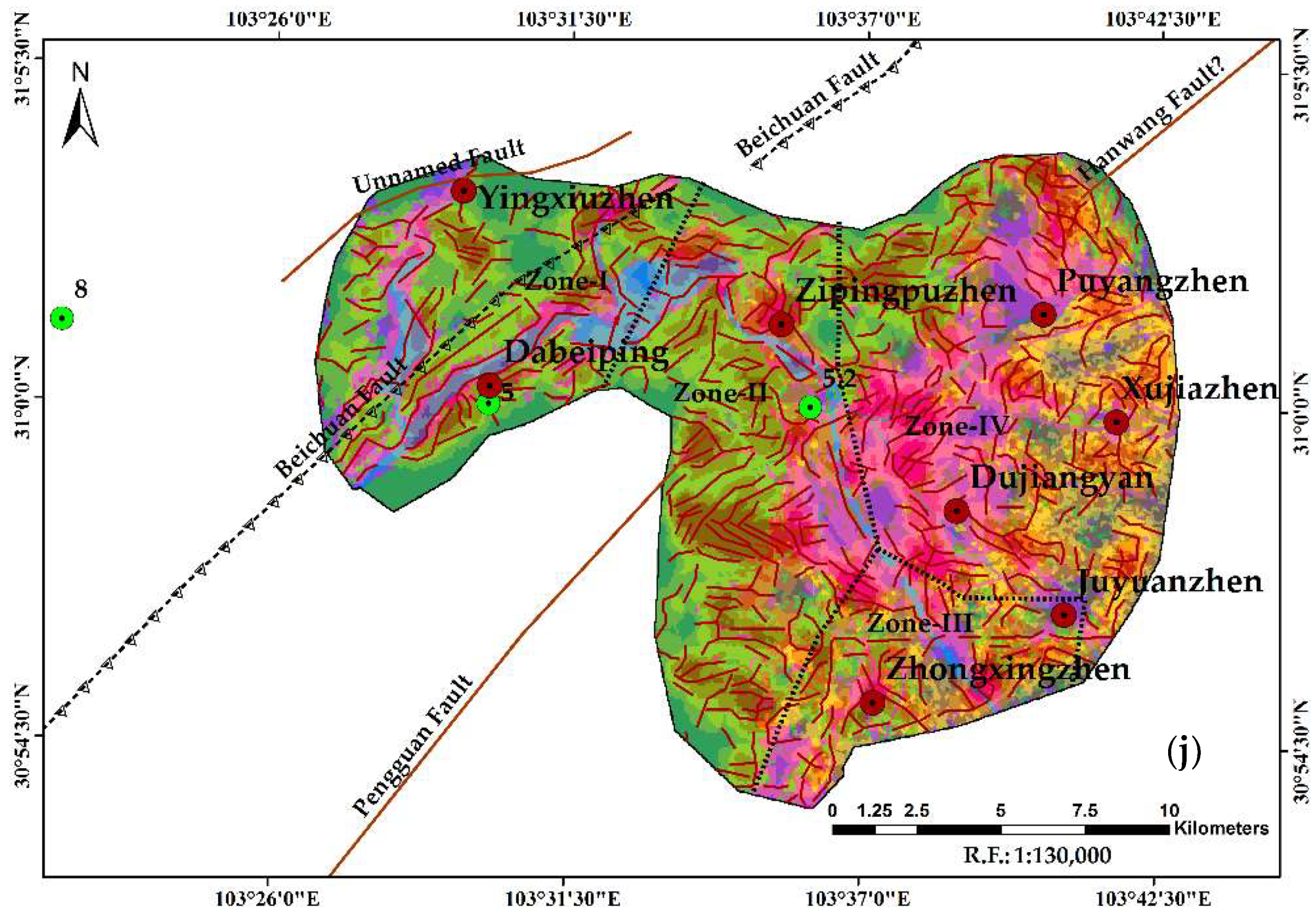
- Lineaments were retrieved digitally by using a sufficient values of LINE algorithm parameters of PCI Geomatica 16.0 version software. The default parameters of the LINE algorithm were modified as an image, considering a small area rather than the whole satellite scene. Various computer-aided methods, such as edge detection, thresholding, and curve extraction steps, were carried out over derived PCA images (i.e., PC1 best band chosen) of Landsat 5 TM and Landsat 8 OLI data sets of three different times such as, 2007, 2008, and 2018, respectively.
- Six parameters RADI-(10), GTHR-(15), LTHR-(20), FTHR-(3), ATHR-(15), and DTHR-(10) for lineament feature extraction were carried out. These parameters were saved into a shapefile and imported in ArcGIS for line splitting at vertices, where compound lines were split into simple lines, and the final lineaments were considered.
- In the next stage, LD mapping, the shapefile of the lineament data was exported and saved in the CADdxf file format, which was then used for lineament direction measurement by creating a rose diagram in the RockWorks 17 software environment.
3. Results
3.1. Dynamic Characteristics of LULC Change Monitoring
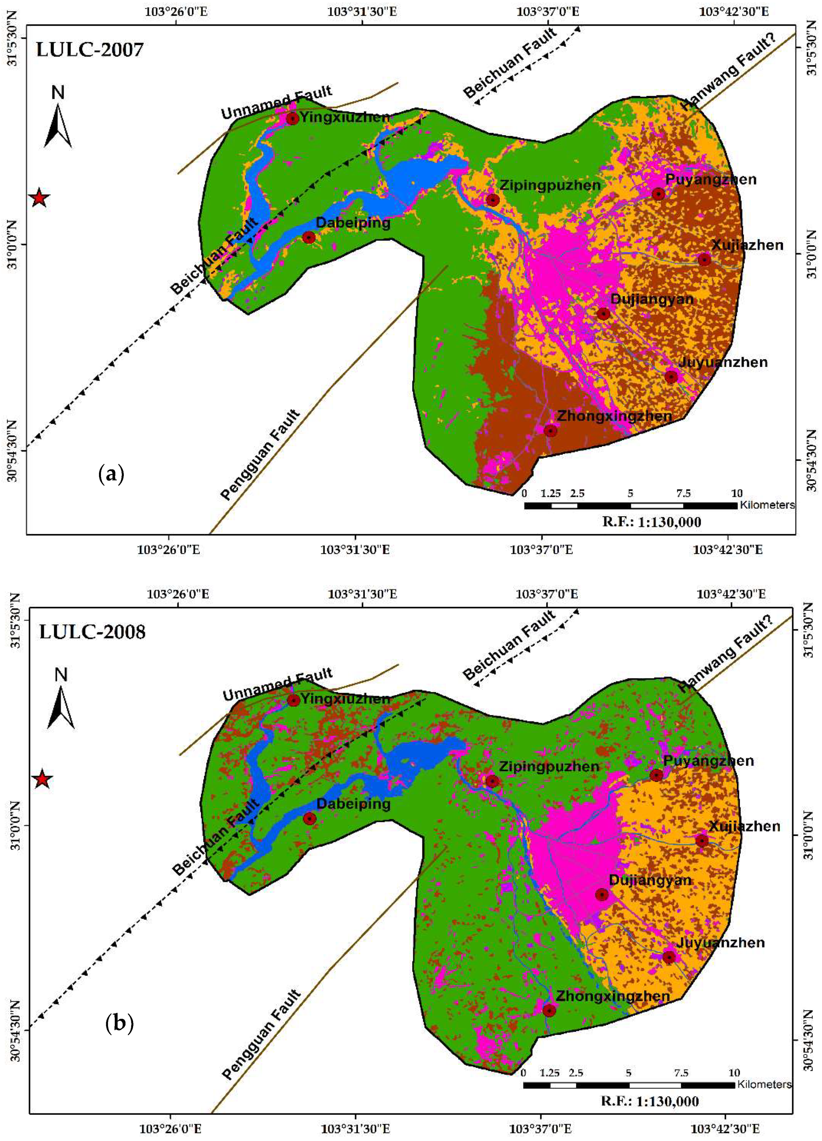
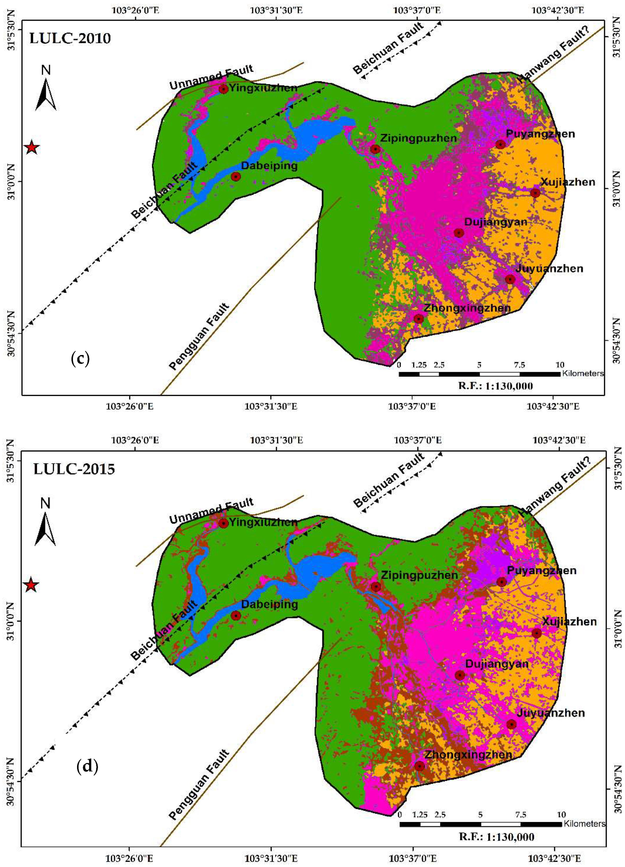
3.1.1. LULC Mapping, Accuracy Assessment, and Quantity Change Characteristics
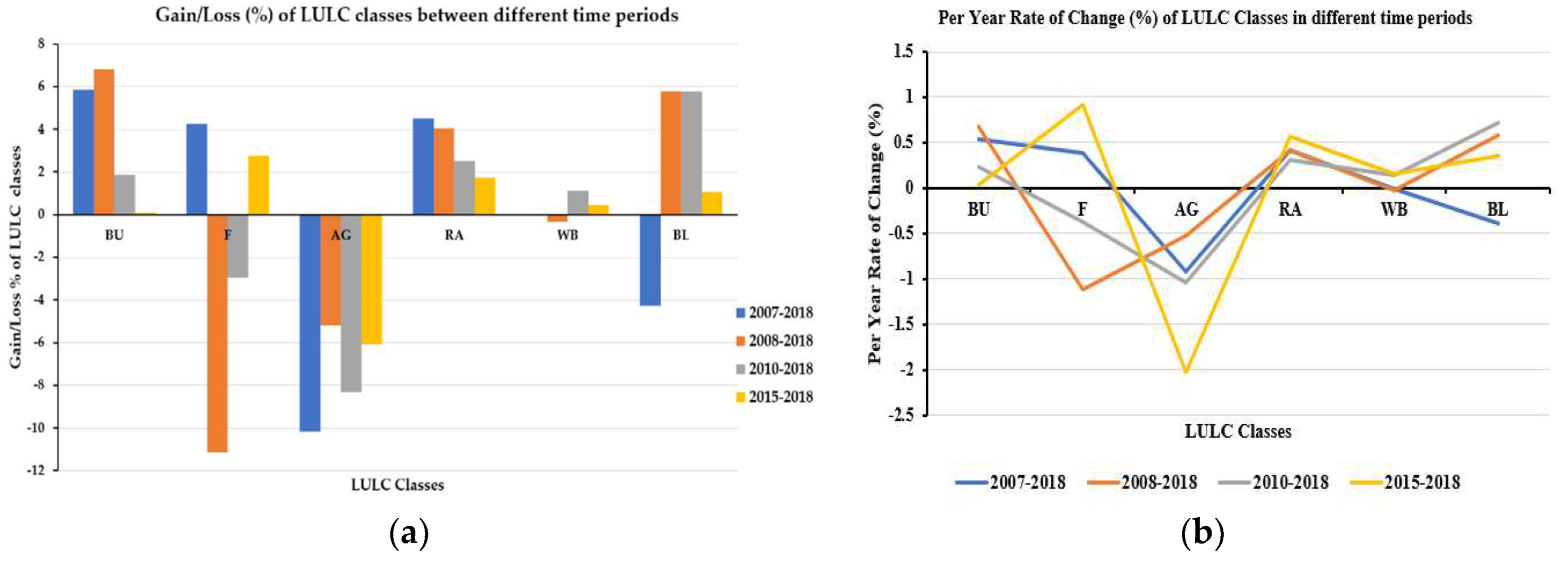
3.1.2. LULC Dynamic Degree, and Gain and Loss Estimations from 2007–2018
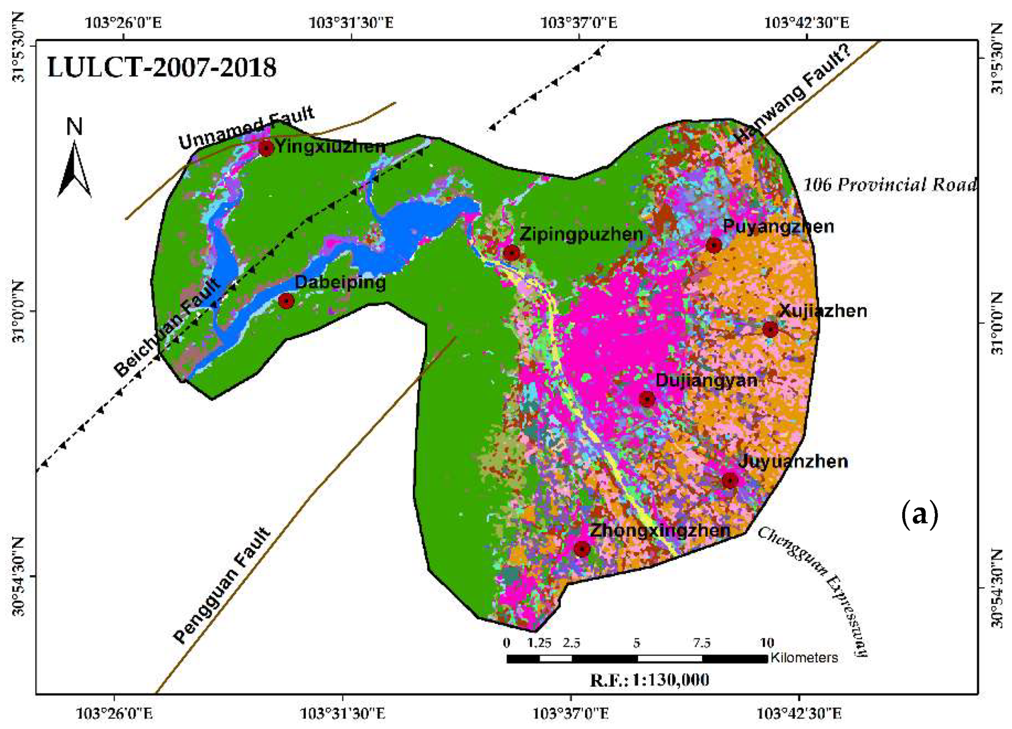
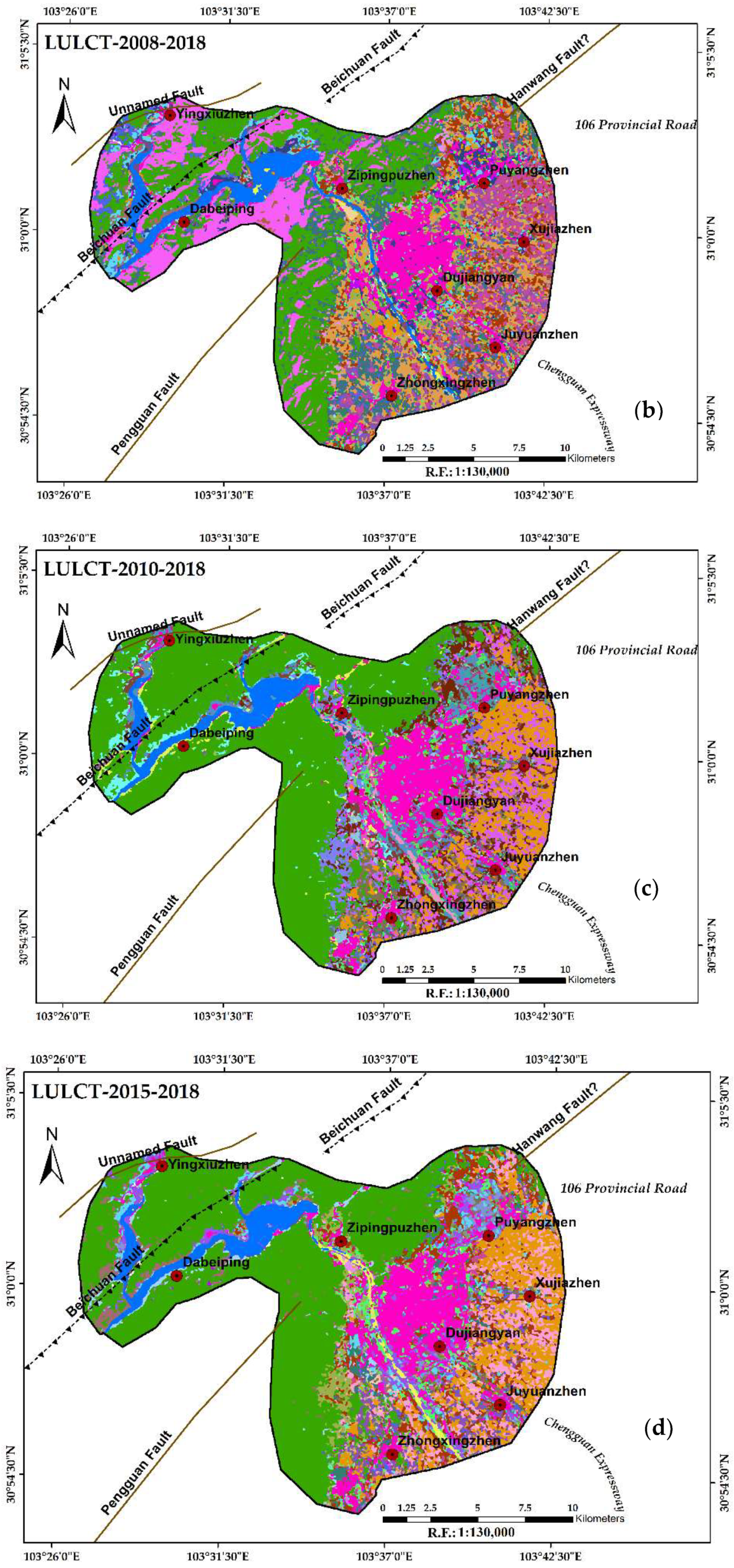
3.2. LULC Transition Mapping and Matrices Calculation
3.3. Landscape Risk Area Indentification
4. Discussion
5. Conclusions
Supplementary Materials
Author Contributions
Funding
Acknowledgments
Conflicts of Interest
References
- Nunes, C.; Auge, J. (Eds.) Land-Use and Land-Cover Change (LUCC): Implementation Strategy; IGBP Report 48 and IHDP Report 10; IGBP Secretariat; Royal Swedish Academy of Science: Stockholm, Sweden, 1999. [Google Scholar]
- Shi, P.; Chen, J.; Pan, Y. Land use change mechanism in Shenzhen city. Acta. Geogr. Sin. 2000, 55, 151–160. (In Chinese) [Google Scholar]
- Pan, D.; Domon, G.; de Blois, S.; Bouchard, A. Temporal (1958–1993) and spatial patterns of land use changes in Haut-Saint-Laurent (Quebec, Canada) and their relation to landscape physical attributes. Lands. Ecol. 1999, 14, 35–52. [Google Scholar] [CrossRef]
- Chen, S.; Zeng, S.; Xie, C. Remote Sensing and GIS for urban growth analysis in China. Photogram. Eng. Remote Sens. 2000, 66, 593–598. [Google Scholar]
- Serra, P.; Pons, X.; Sauri, D. Land-cover and land-use change in a Mediterranean landscape: A spatial analysis of driving forces integrating biophysical and human factors. Appl. Geogr. 2008, 28, 189–209. [Google Scholar] [CrossRef]
- Nunes, A.N.; Almeida, A.C.D.; Coelho, C.O.A. Impacts of land use and cover type on runoff and soil erosion in a marginal area of Portugal. Appl. Geogr. 2011, 31, 687–699. [Google Scholar] [CrossRef]
- König, H.J.; Uthes, S.; Schuler, J.; Zhen, L.; Purushothaman, S.; Suarma, U.; Sghaier, M.; Makokha, S.; Helming, K.; Sieber, S.; et al. Regional impact assessment of land use scenarios in developing countries using the FoPIA approach: Findings from five case studies. J. Environ. Manag. 2013, 127, S56–S64. [Google Scholar] [CrossRef] [PubMed]
- Tendaupenyu, P.; Magadza, C.H.D.; Murwira, A. Changes in landuse/landcover patterns and human population growth in the Lake Chivero catchment, Zimbabwe. Geocarto Int. 2017, 32, 1–34. [Google Scholar] [CrossRef]
- Li, H.; Xiao, P.; Feng, X.; Yang, Y.; Wang, L.; Zhang, W.; Wang, X.; Feng, W.; Chang, X. Using Land Long-term Data Records to Map Land Cover Changes in China Over 1981–2010. IEEE J. Select. Topics Appl. Earth Obs. Remote Sens. 2017, 10, 1372–1389. [Google Scholar] [CrossRef]
- Martínez, S.; Mollicone, D. From Land Cover to Land Use: A Methodology to Assess Land Use from Remote Sensing Data. Remote Sens. 2012, 4, 1024–1045. [Google Scholar] [CrossRef]
- Tiwari, M.K.; Saxena, A. Change detection of land use/landcover pattern in an around Mandideep and Obedullaganj area, using remote sensing and GIS. Int. J. Technol. Eng. Syst. 2011, 2, 398–402. [Google Scholar]
- Liu, J.Y.; Kuang, W.H.; Zhang, Z.X.; Xu, X.L.; Qin, Y.W.; Ning, J.; Zhou, W.C.; Zhang, S.W.; Li, R.D.; Yan, C.Z.; et al. Spatiotemporal characteristics, patterns and causes of land use changes in China since the late 1980s. J. Geogr. Sci. 2014, 24, 195–210. [Google Scholar] [CrossRef]
- Liu, J.; Zhang, Z.; Xu, X.; Kuang, W.; Zhou, W.; Zhang, S.; Li, R.; Yan, C.; Yu, D.; Wu, S.; et al. Spatial patterns and driving forces of land use change in China during the early 21st century. J. Geogr. Sci. 2010, 20, 483–494. [Google Scholar] [CrossRef]
- Liu, J.Y.; Liu, M.L.; Zhuang, D.F.; Zhang, Z.X.; Deng, X.Z. Study on spatial pattern of land-use change in China during 1995–2000. Sci. China Earth Sci. 2003, 46, 373–384. [Google Scholar]
- Lambin, E. The causes of land-use and land-cover change moving beyond the myths. Global Environ. Chang 2001, 11, 261–269. [Google Scholar] [CrossRef]
- Lambin, E.F.; Geist, H.J.; Lepers, E. Dynamics of land-use and land-cover change in tropical regions. Ann. Rev. Env. Resour. 2003, 28, 205–241. [Google Scholar] [CrossRef]
- Lambin, E.F.; Geist, H.J. Land-Use and Land-Cover Change: Local Processes and Global Impacts; Springer: Berlin/Heidelberg, Germany, 2006. [Google Scholar]
- Zhang, M. Progress of land science centered on land use / land cover change. Adv. Geogr. 2001, 20, 297–304. (In Chinese) [Google Scholar]
- Zhang, Y.L.; Li, X.B.; Fu, X.F.; Xie, G.D.; Zheng, D. Urban land use change in Lhasa. Acta. Geogr. Sin. 2000, 55, 395–406. [Google Scholar]
- Tahir, M.; Imam, E.; Tahir, H. Evaluation of land use/land cover changes in Mekelle City, Ethiopia using Remote Sensing and GIS. Comput. Ecol. Soft. 2013, 3, 9–16. [Google Scholar]
- Li, F.; Liu, G. Characterizing Spatiotemporal Pattern of Land Use Change and Its Driving Force Based on GIS and Landscape Analysis Techniques in Tianjin during 2000–2015. Sustainability 2017, 9, 1–26. [Google Scholar] [CrossRef]
- Ying, C.; Ling, H.; Kai, H. Change and Optimization of Landscape patterns in a Basin Based on Remote Sensing Images: A Case Study in China. Pol. J. Environ. Stud. 2017, 26, 2343–2353. [Google Scholar] [CrossRef]
- Jaafari, S.; Sakieh, Y.; Shabani, A.A.; Danehkar, A.; Nazarisamani, A. Landscape change assessment of reservation areas using remote sensing and landscape metrics (case study: Jajroud reservation, Iran). Environ. Dev. Sustain. 2015, 17, 1–17. [Google Scholar] [CrossRef]
- Seto, K.C.; Fragkias, M. Quantifying spatiotemporal patterns of urban land-use change in four cities of China with time series landscape metrics. Lands. Ecol. 2005, 20, 871–888. [Google Scholar] [CrossRef]
- Fichera, C.R.; Modica, G.; Pollino, M. Land Cover classification and change-detection analysis using multi-temporal remote sensed imagery and landscape metrics. Eur. J. Remote Sens. 2012, 45, 1–18. [Google Scholar] [CrossRef]
- Herold, M.; Scepan, J.; Clarke, K.C. The Use of Remote Sensing and Landscape Metrics to Describe Structures and Changes in Urban Land Uses. Environ. Plan. 2002, 34, 1443–1458. [Google Scholar] [CrossRef]
- Nurwanda, A.; Zain, A.F.M.; Rustiadi, E. Analysis of land cover changes and landscape fragmentation in Batanghari Regency, Jambi Province. In Procedia-Social and Behavioral Sciences, CITIES 2015 International Conference, Intelligent Planning Towards Smart Cities, CITIES 2015, Surabaya, Indonesia, 3–4 November 2015; Elsevier Ltd.: Amsterdam, The Netherlands, 2016; Volume 227, pp. 87–94. [Google Scholar]
- Nagendra, H.; Munroe, D.K.; Southworth, J. From pattern to process: Landscape fragmentation and theanalysis of land use/land cover change. Agric. Ecosyst. Environ. 2004, 101, 111–115. [Google Scholar] [CrossRef]
- Li, R.; Dong, M.; Cui, J.; Zhang, L.; Cui, Q.; He, W. Quantification of the impact of land-use changes on ecosystem services: A case study in Pingbian County. China. Environ. Monit. Assess. 2007, 128, 503–510. [Google Scholar] [CrossRef]
- Schirpke, U.; Kohler, M.; Leitinger, G.; Fontana, V.; Tasser, E.; Tappeiner, U. Future impacts of changing land-use and climate on ecosystem services of mountain grassland and their resilience. Ecosyst. Serv. 2017, 26, 79–94. [Google Scholar] [CrossRef]
- Tasser, E.; Leitinger, G.; Tappeiner, U. Climate change versus land-use change—What affects the mountain landscapes more? Land Use Policy 2017, 60, 60–72. [Google Scholar] [CrossRef]
- Nath, B.; Acharjee, S. Urban Municipal Growth and Landuse Change Monitoring Using High Resolution Satellite Imageries and Secondary Data: A Geospatial Study on Kolkata Municipal Corporation, Kolkata, India. Stud. Sur. Mapp. Sci. 2013, 3, 43–54. [Google Scholar]
- Bhagawat, R. Urban Growth and Land Use/Land Cover Change of Pokhara Sub-metropolitan city, Nepal. J. Theor. Appl. Inf. Technol. 2011, 26, 118–129. [Google Scholar]
- Dewan, A.M.; Yamaguchi, Y. Land use and land cover change in Greater Dhaka, Bangladesh: Using remote sensing to promote sustainable urbanization. Appl. Geogr. 2009, 29, 390–401. [Google Scholar] [CrossRef]
- Sui, L.Y.; Ming, C.B. The study framework of land use/cover change based on sustainable development in China. Geogr. Res. 2002, 21, 324–330. [Google Scholar]
- Ellis, E. Land-use and Land-cover Change. In: Encyclopedia of Earth; Cutler, J., Ed.; Environmental Information Coalition, National Council for Science and the Environment: Washington, DC, USA, 2010; Available online: http://www.eoearth.org/article/Landuseandland-coverchange (accessed on 5 December 2010).
- Collins English Dictionary. Definition of ‘Transition’. Available online: https://www.collinsdictionary.com/dictionary/english/transition (accessed on 18 November 2018).
- Su, C.H.; Fu, B.J.; Lu, Y.H.; Lu, N.; Zeng, Y.; He, A.; Lamparski, H.L. Land use change and anthropogenic driving force: A case study in Yanhe River Basin. Chin. Geogr. Sci. 2011, 21, 587–599. [Google Scholar] [CrossRef]
- Chang, Y.; Hou, K.; Li, X.; Zhang, Y.; Chen, P. Review of Land Use and Land Cover Change research progress. IOP Conf. Ser. Earth Environ. Sci. 2018, 113, 1–6. [Google Scholar] [CrossRef]
- Tang, H. Research progress of land use/land cover change (LUCC) model. J. Geogr. 2009, 64, 456–468. (In Chinese) [Google Scholar]
- Xiubin, L. A review of the international researches on land use and land cover change. Acta Geogr. Sin. 1996, 25, 344–356. [Google Scholar]
- Yun, H. A study on land use/cover change the need for a new integrated approach. J. Geogr. Res. 2011, 20, 645–652. [Google Scholar]
- Seto, K.C.; Woodcock, C.E.; Song, C.; Huang, X.; Lu, J.; Kaufmann, R.K. Monitoring land-use change in the Pearl River Delta using Landsat TM. Int. J. Remote Sens. 2002, 23, 1985–2004. [Google Scholar] [CrossRef]
- Liu, M.; Hu, Y.; Chang, Y.; He, X.; Zhang, W. Land use and land cover change analysis and prediction in the upper reaches of the Minjiang River, China. Environ. Manag. 2009, 43, 899–907. [Google Scholar] [CrossRef]
- Sleeter, B.M.; Sohi, T.L.; Loveland, T.R.; Auch, R.F.; Acevedo, W.; Drummond, M.A.; Sayler, K.L.; Stehman, S.V. Land-cover change in the conterminous United States from 1973–2000. Glob. Environ. Chang. 2013, 23, 733–748. [Google Scholar] [CrossRef]
- Sleeter, B.M.; Liu, J.; Daniel, C.; Rayfield, B.; Serba, J.; Hawbaker, T.J.; Zhu, Z.; Selmants, P.C.; Loveland, T.R. Effects of contemporary land-use and land-cover change on the Carbon balance of terrestrial ecosystems in the United States. Environ. Res. Lett. 2018, 13, 045006. [Google Scholar] [CrossRef]
- Latifovic, R.; Pouliot, D.; Olthof, I. Circa 2010 Land Cover of Canada: Local Optimization Methodology and Product Development. Remote Sens. 2017, 9, 1098. [Google Scholar] [CrossRef]
- NOAA. What is the Difference between Land Cover and Land Use? National Ocean Service Website. Available online: https://oceanservice.noaa.gov/facts/lclu.html (accessed on 23 November 2018).
- European Environment Agency. Landscape in Transition, An Account of 25 Years of Land Cover Change in Europe; Publications Office of the European Union: Luxembourg, 2017; Available online: https://www.eea.europa.eu/publications/landscapes-in-transition (accessed on 5 December 2018).
- Tali, J.A.; Divya, S.; Murthy, K. Influence of urbanization on the land use change: A case study of Srinagar City. Am. J. Res. Comm. 2013, 1, 271–283. [Google Scholar]
- Rawat, J.S.; Kumar, M. Monitoring Land Use/Cover Change Using Remote Sensing and GIS Techniques: A Case Study of Hawalbagh Block, District Almora, Uttarakhand, India. Egypt. J. Remote Sens. Space Sci. 2015, 18, 77–84. [Google Scholar] [CrossRef]
- Appiah, D.O.; Schroeder, D.; Forkuo, E.K.; Bugri, J.T. Application of Geo-Information Techniques in Land Use and Land Cover Change Analysis in a Peri-Urban District of Ghana. Inter. J. Geo-Inf. 2015, 4, 1265–1289. [Google Scholar] [CrossRef]
- Yu, D.; Srinivasan, S. Urban land use change and regional access: A case study in Beijing, China. Habitat Int. 2016, 51, 103–113. [Google Scholar]
- Mundia, C.N.; Aniya, M. Dynamics of land use/cover changes and degradation of Nairobi City, Kenya. Land Degrad. Dev. 2010, 17, 97–108. [Google Scholar] [CrossRef]
- Li, Y.; Zhang, Q. Human-environment interactions in China: Evidence of land-use change in Beijing-Tianjin-Hebei Metropolitan Region. Hum. Ecol. Rev. 2013, 20, 26–35. [Google Scholar]
- Dewan, A.M.; Yamaguchi, Y. Using remote sensing and GIS to detect and monitor land use and land cover change in Dhaka Metropolitan of Bangladesh during 1960–2005. Environ. Monit. Assess. 2009, 150, 237–249. [Google Scholar] [CrossRef]
- Lo, C.P.; Yang, X. Drivers of Land-Use/Land-Cover Changes and Dynamic Modeling for the Atlanta, Georgia Metropolitan Area. Photogramm. Eng. Remote Sens. 2002, 68, 1073–1082. [Google Scholar]
- Butt, A.; Shabbir, R.; Ahmad, S.S.; Aziz, N. Land use change mapping and analysis using Remote Sensing and GIS: A case study of Simly watershed, Islamabad, Pakistan. Egypt. J. Remote Sens. Space Sci. 2015, 18, 251–259. [Google Scholar] [CrossRef]
- Malik, M.I.; Bhat, M.S. Integrated Approach for Prioritizing Watersheds for Management: A Study of Lidder Catchment of Kashmir Himalayas. Environ. Manag. 2015, 54, 1267–1287. [Google Scholar] [CrossRef]
- Kaliraj, S.; Chandrasekar, N.; Ramachandran, K.K.; Srinivas, Y.; Saravanan, S. Coastal land use and land cover change and transformations of Kanyakumari coast, India using remote and GIS. Egypt. J. Remote Sens. Space Sci. 2017, 20, 169–185. [Google Scholar]
- Islam, K.; Jashimuddin, M.; Nath, B.; Nath, T.K. Land use classification and change detection by using multi-temporal remotely sensed imagery: The case of Chunati wildlife sanctuary, Bangladesh. Egypt. J. Remote Sens. Space Sci. 2018, 21, 37–47. [Google Scholar] [CrossRef]
- Singh, R.P.; Sahoo, A.K.; Bhoi, S.; Kumar, M.G.; Bhuiyan, C.S. Ground deformation of Gujarat earthquake of 26 January 2001. J. Geol. Soc. India 2001, 58, 209–214. [Google Scholar]
- Singh, R.P.; Bhoi, S.; Sahoo, A.K.; Raj, U.; Ravindran, S. Surface manifestations after the Gujarat earthquake. Curr. Sci. 2001, 81, 164–166. [Google Scholar]
- Singh, R.P.; Bhoi, S.; Sahoo, A.K. Significant changes in the ocean parameters after the Gujarat earthquake. Curr. Sci. 2001, 80, 1376–1377. [Google Scholar]
- Singh, R.; Simon, B.; Joshi, P.C. Estimation of surface latent heat fluxes from IRSP4/MSMR satellite data. Proc. Indian Acad. Sci. Earth Planet. Sci. 2001, 110, 231–238. [Google Scholar]
- Singh, R.P.; Bhoi, S.; Sahoo, A.K. Changes observed on land and ocean after Gujarat earthquake 26 January 2001 using IRS data. Int. J. Remote Sens. 2002, 23, 3123–3128. [Google Scholar] [CrossRef]
- Dey, S.; Singh, R.P. Surface Latent Heat Flux as an earthquake precursor. Nat. Hazards Earth Syst. Sci. 2003, 3, 749–755. [Google Scholar] [CrossRef]
- Okada, Y.; Mukai, S.; Singh, R.P. Changes in atmospheric aerosol parameters after Gujarat earthquake of January 26 2001. Adv. Space Res. 2004, 33, 254–258. [Google Scholar] [CrossRef]
- Dey, S.; Sarkar, S.; Singh, R.P. Anomalous changes in column water vapor after Gujarat earthquake. Adv. Space Res. 2004, 33, 274–278. [Google Scholar] [CrossRef]
- Singh, V.P.; Singh, R.P. Changes in stress pattern around epicentral region of Bhuj earthquake of 26 January 2001. Geophys. Res. Lett. 2005, 32, 1–4. [Google Scholar] [CrossRef]
- Singh, R.P.; Mehdi, W.; Gautam, R.; Kumar, J.S.; Zlotnicki, J.; Kafatos, M. Precursory signals using satellite and ground data associated with the Wenchuan Earthquake of 12 May 2008. Int. J. Remote Sens. 2010, 31, 3341–3354. [Google Scholar] [CrossRef]
- Balz, T.; Liao, M. Building-damage detection using post-seismic high-resolution SAR satellite data. Int. J. Remote Sens. 2010, 31, 3369–3391. [Google Scholar] [CrossRef]
- Guo, H.; Ma, J.; Zhang, B.; Li, Z.; Huang, J.; Zhu, L. Damage consequence chain mapping after the Wenchuan Earthquake using remotely sensed data. Int. J. Remote Sens. 2010, 31, 3427–3433. [Google Scholar] [CrossRef]
- Sowter, A. Orthorectification and interpretation of differential InSAR data over mountainous areas: A case study of the May 2008 Wenchuan Earthquake. Int. J. Remote Sens. 2010, 31, 3435–3448. [Google Scholar] [CrossRef]
- Zhuang, J.Q.; Cui, P.; Ge, Y.G.; He, Y.P.; Liu, Y.H.; Guo, X.J. Probability assessment of river blocking by debris flow associated with the Wenchuan Earthquake. Int. J. Remote Sens. 2010, 31, 3465–3478. [Google Scholar] [CrossRef]
- Pan, G.; Tang, D. Damage information derived from multi-sensor data of the Wenchuan Earthquake of May 2008. Int. J. Remote Sens. 2010, 31, 3509–3519. [Google Scholar] [CrossRef]
- Zhuang, W.; Lin, J.; Peng, J.; Lu, Q. Estimating Wenchuan Earthquake induced landslides based on remote sensing. Int. J. Remote Sens. 2010, 31, 3495–3508. [Google Scholar] [CrossRef]
- Wu, F.; Yu, B.; Yan, M.; Wang, Z. Eco-environmental research on the Wenchuan Earthquake area using Disaster Monitoring Constellation (DMC) Beijing-1 small satellite images. Int. J. Remote Sens. 2010, 31, 3643–3660. [Google Scholar] [CrossRef]
- Singh, R.P. Satellite observations of the Wenchuan Earthquake, 12 May 2008. Int. J. Remote Sens. 2010, 31, 3335–3339. [Google Scholar] [CrossRef]
- Ahmad, R.A.; Singh, R.P.; Adris, A. Seismic hazard assessment of Syria using seismicity, DEM, slope, active faults, and GIS. Remote Sens. Appl. Soc. Environ. 2017, 6, 59–70. [Google Scholar] [CrossRef]
- Pôças, I.; Cunha, M.; Pereira, L.S. Remote sensing-based indicators of changes in a mountain rural landscape of Northeast Portugal. Appl. Geogr. 2011, 31, 871–880. [Google Scholar] [CrossRef]
- Yi, Y.; Zhao, Y.Z.; Ding, G.D.; Cao, Y. Effects of urbanization on landscape patterns in a mountainous area: A Case Study in the Mentougou District, Beijing, China. Sustainability 2016, 8, 1190. [Google Scholar] [CrossRef]
- Jain, S.; Laphawan, S.; Singh, P.K. Tracing the Changes in the Pattern of Urban Landscape of Dehradun over Last Two Decades using RS and GIS. Int. J. Adv. Remote Sens. GIS 2013, 2, 351–362. [Google Scholar]
- Mottet, A.; Ladet, S.; Coque, N.; Gibon, A. Agricultural land-use change and its drivers in mountain landscapes: A case study in the Pyrenees. Agric. Ecosyst. Environ. 2006, 114, 296–310. [Google Scholar] [CrossRef]
- Arellano-Baeza, A.A.; Zverev, A.; Malinnikov, V. Study of Changes in the lineament structure, caused by earthquakes in South America by applying the lineament analysis to the ASTER (Terra) satellite data. Adv. Space Res. 2004, 33, 274–278. [Google Scholar] [CrossRef]
- Bardhan, R.; Debnath, R.; Bandopadhyay, S. A conceptual model for identifying the risk susceptibility of urban green spaces using geo-spatial techniques. Model. Earth Syst. Environ. 2016, 2, 144. [Google Scholar] [CrossRef]
- Ingram, K.; Knapp, E.; Robinson, J.W. Change Detection Technique Development for Improved Urbanized Area Delineation; Technical Memorandum CSC/TM-81/6087; Computer Sciences Corporation: Silver Springs, MD, USA, 1981. [Google Scholar]
- Teixeira, Z.; Teixeira, H.; Marques, J.C. Systematic processes of land use/land cover change to identify relevant driving forces: Implications on water quality. Sci. Total Environ. 2014, 470–471, 1320–1335. [Google Scholar] [CrossRef]
- Jensen, J.R. Remote Sensing of the Environment: An Earth Resource Perspective 2/e; Pearson Education India: Noida, India, 2009; Volume 47. [Google Scholar]
- Richards, J.; Jia, X. Remote Sensing Digital Image Analysis; Springer: Berlin/Heidelberg, Germany, 1999. [Google Scholar]
- United Nations (UN). Transforming Our World: The 2030 Agenda for Sustainable Development. Resolution Adopted by the General Assembly on 25 September 2015. Available online: http://www.un.org/ga/search/view doc.asp? Symbol=A/RES/70/1 & Lang=E (accessed on 17 November 2018).
- USGS Earth Explorer Landsat archive (2007–2018). Available online: https://earthexplorer.usgs.gov (accessed on 10 February 2018).
- FAO. Global Forest Resources Assessment 2015: Terms and Definitions; Forest Resources Assessment Programme Working Paper 180; FAO Forestry Department: Rome, Italy, 2012. [Google Scholar]
- Turner, B.L.; Meyer, W.B.; Skole, D.L. Global land-use/landcover change: Towards an integrated study. Ambio Stockholm 1994, 23, 91–95. [Google Scholar]
- Tekle, K.; Hedlund, L. Land cover changes between 1958 and 1986 in Kalu District, southern Wello, Ethiopia. Mt. Res. Dev. 2000, 20, 42–51. [Google Scholar] [CrossRef]
- Anderson, J.R.; Hardy, E.E.; Roach, J.T.; Witmer, R.E. A Land Use and Land Cover Classification for Use with Remote Sensor Data (USGS Professional Paper 964); U.S. Government Printing Office: Washington, DC, USA, 1976; p. 18.
- Singh, A.; Singh, S.; Garga, P.K.; Khanduri, K. Land Use and Land Cover Change Detection: A Comparative Approach using Post Classification Change Matrix Function Change Detection Methodology of Allahabad City. Int. J. Curr. Eng. Technol. 2013, 3, 142–148. [Google Scholar]
- Tudes, S.; Yigiter, N.D. Preparation of land use planning model using GIS based on AHP: Case study Adana-Turkey. Bull. Eng. Geol. Environ. 2010, 69, 235–245. [Google Scholar] [CrossRef]
- Data Catalog-Data.Gov. Shapefile: Generalized Geology of the Far East (geo3al). Metadata creation date: 18 March 2005. Available online: https://catalog.data.gov/dataset/generalized-geology-of-the-far-east-geo3al (accessed on 15 February 2018).
- Tang, R.C.; Han, W.B. Active Faults and Earthquakes in Sichuan; Seismological Press: Beijing, China, 1993; pp. 1–368. (In Chinese) [Google Scholar]
- Densmore, A.L.; Ellis, M.A.; Li, Y.; Zhou, R.J.; Hancock, G.S.; Richardson, N. Active tectonics of the Beichuan and Pengyuan faults at the eastern margin of the Tibetan plateau. Tectonics 2007, 26, TC4005. [Google Scholar] [CrossRef]
- Hubbard, J.; Shaw, J.H. Uplift of the Longmen Shan and Tibetan Plateau, and the 2008 Wenchuan (M = 7.9) earthquake. Nature 2009, 458, 194–197. [Google Scholar] [CrossRef]
- Ran, Y.; Shi, X.; Wang, H.; Chen, L.; Chen, J.; Liu, R.; Gong, H. The maximum vertical co-seismic displacement and the style of deformation associated with the 2008 Wenchuan earthquake. Chin. Sci. Bull. 2010, 54, 841–850. [Google Scholar] [CrossRef]


| SL. No. | Satellite Sensors | Image Acquisition Time | Path/Row | Resolution (m) | Image Type |
|---|---|---|---|---|---|
| 1 | Landsat 5 TM | 18 September 2007 | 130/38 | 30 | Level-1 GeoTIFF |
| 2 | Landsat 5 TM | 7 November 2008 | 130/38 | 30 | Level-1 GeoTIFF |
| 3 | Landsat 5 TM | 29 January 2010 | 130/38 | 30 | Level-1 GeoTIFF |
| 4 | Landsat 8 OLI | 12 February 2015 | 130/38 | 30 | Level-1 GeoTIFF |
| 5 | Landsat 8 OLI | 19 January 2018 | 130/38 | 30 | Level-1 GeoTIFF |
| SL. No. | LULC Classes | General Descriptions |
|---|---|---|
| 1 | BU | All residential, commercial and industrial areas, continuous, and non-continuous urban and rural fabrics, transportation infrastructure |
| 2 | F | Shrubs and semi-natural vegetation transitional land, natural vegetation, urban green areas |
| 3 | AG | Arable land, permanent crops, and heterogeneous agricultural areas, intensively, moderately and sparsely cultivated lands |
| 4 | RA | Previous damaged buildings areas, Newly constructed land areas for buildings and transport |
| 5 | WB | Inland water bodies, generally including major rivers, lakes, ponds, and water reservoirs |
| 6 | BL | Land-exposed soils, sand, rocks, or snow, land due to earthquake-induced landslides, open areas, grazing land areas, less than 10% vegetated cover during any time of the year |
| Total Area Coverage (km2) | DD (%) between Different Times | ||||||||
|---|---|---|---|---|---|---|---|---|---|
| LULC Classes | 2007 | 2008 | 2010 | 2015 | 2018 | 2007–2018 | 2008–2018 | 2010–2018 | 2015–2018 |
| BU | 40.54 | 37.41 | 53.23 | 58.84 | 59.13 | 4.17 | 5.81 | 1.39 | 0.16 |
| F | 125.71 | 174.73 | 148.63 | 130.45 | 139.25 | 0.98 | −2.03 | −0.79 | 2.25 |
| AG | 63.01 | 47.22 | 57.12 | 50.08 | 30.66 | −4.67 | −3.51 | −5.79 | −12.93 |
| RA | 2.01 | 3.36 | 8.32 | 10.83 | 16.29 | 64.59 | 38.48 | 11.97 | 16.80 |
| WB | 17.60 | 18.17 | 13.54 | 15.65 | 17.14 | −0.24 | −0.57 | 3.32 | 3.17 |
| BL | 69.43 | 37.41 | 37.46 | 52.45 | 55.83 | −1.78 | 4.92 | 6.13 | 2.15 |
| Total Area Coverage (%) | Gain/Loss (%) between Different Times | ||||||||
|---|---|---|---|---|---|---|---|---|---|
| LULC Classes | 2007 | 2008 | 2010 | 2015 | 2018 | 2007–2018 | 2008–2018 | 2010–2018 | 2015–2018 |
| BU | 12.74 | 11.75 | 16.72 | 18.49 | 18.58 | 5.84 | 6.83 | 1.86 | 0.09 |
| F | 39.49 | 54.90 | 46.70 | 40.98 | 43.75 | 4.26 | −11.15 | −2.95 | 2.77 |
| AG | 19.80 | 14.83 | 17.95 | 15.73 | 9.63 | −10.17 | −5.20 | −8.32 | −6.10 |
| RA | 0.63 | 1.06 | 2.61 | 3.40 | 5.12 | 4.49 | 4.06 | 2.51 | 1.72 |
| WB | 5.53 | 5.71 | 4.25 | 4.92 | 5.38 | −0.05 | −0.33 | 1.13 | 0.46 |
| BL | 21.81 | 11.75 | 11.77 | 16.48 | 17.54 | −4.27 | 5.79 | 5.77 | 1.06 |
| Total | 100.00 | 100.00 | 100.00 | 100.00 | 100.00 | 100.00 | 100.00 | 100.00 | 100.00 |
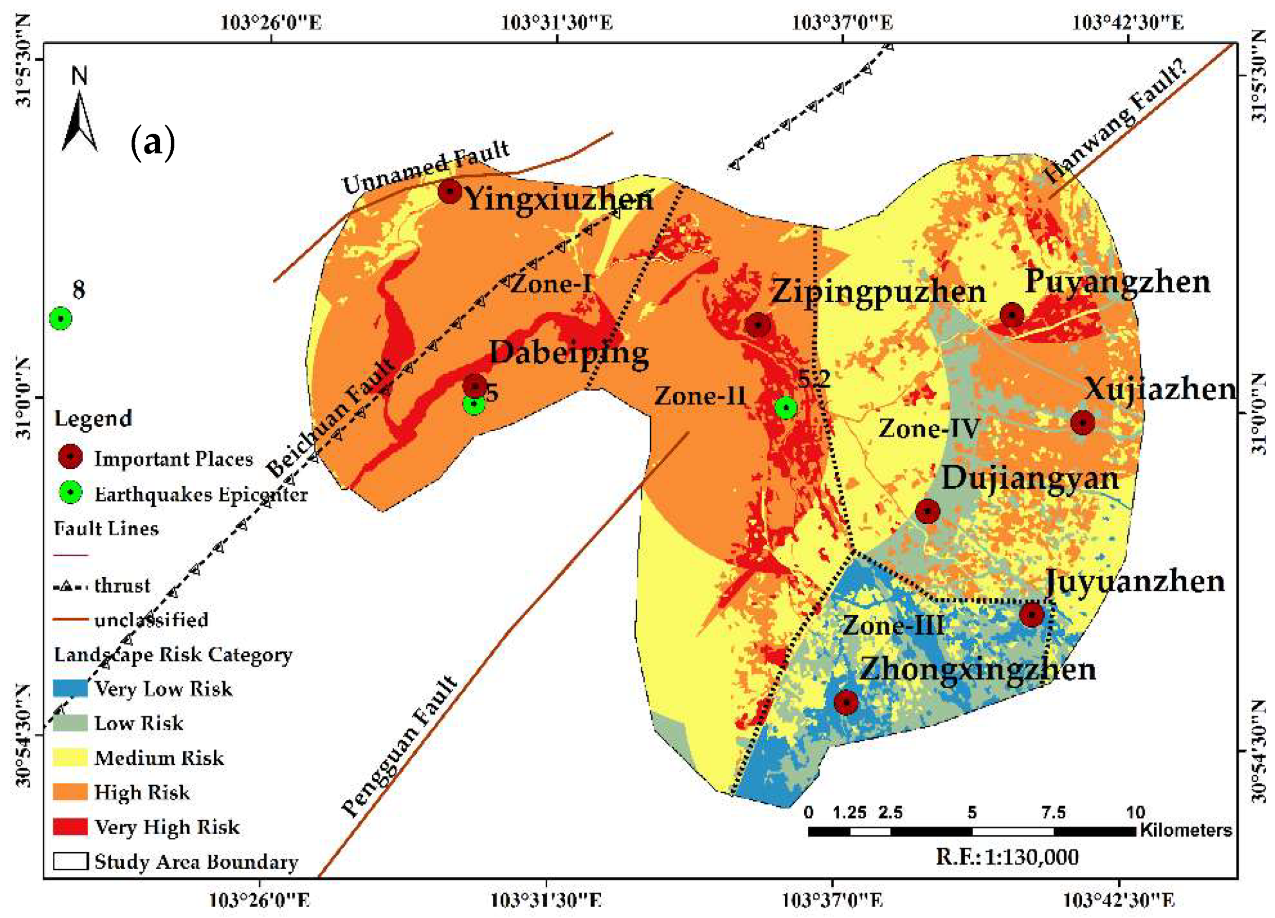
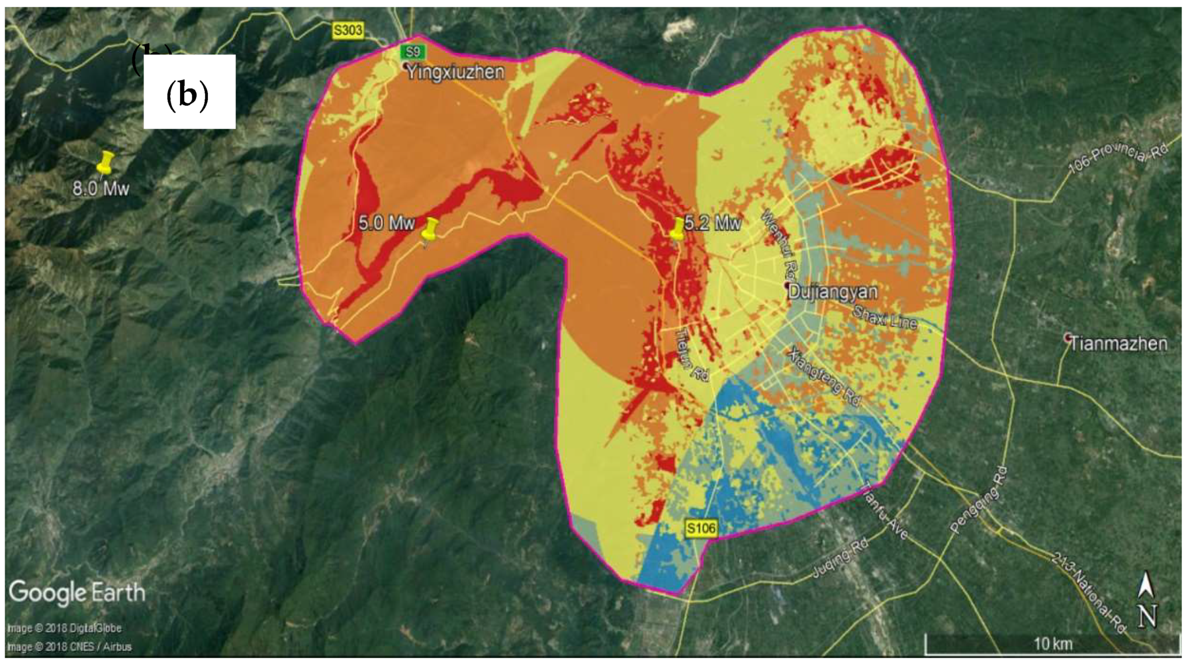
| Total Risk Weight Class Range | Risk Category | Risk Area (km2) | Risk Area (%) | Geological Zone Under Risk | Landscape Type Under Risk (Priority Based) | Important Locations Under Risk |
|---|---|---|---|---|---|---|
| 14–16 | Very Low | 14.62 | 4.59 | Zones III, IV | F, WB, BU, RA | 8, 7, 6 |
| 17–18 | Low | 9.54 | 3.00 | Zones II, III, IV | F, WB, BU, BL, AG | 8, 4, 6, 5 |
| 19–20 | Medium | 119.54 | 37.56 | Zones I, II, III, IV | WB, BU, F, AG, BL | 1, 4, 6, 7, 8 |
| 21–22 23–25 | High Very High | 149.23 25.37 | 46.88 7.97 | Zones I, II, IV Zones I, II, IV | BU, F, BL, AG, WB BU, WB, BL, F, AG | 1, 2, 3, 5 2, 3, 4 |
| Total | 318.30 | 100.00 |
© 2018 by the authors. Licensee MDPI, Basel, Switzerland. This article is an open access article distributed under the terms and conditions of the Creative Commons Attribution (CC BY) license (http://creativecommons.org/licenses/by/4.0/).
Share and Cite
Nath, B.; Niu, Z.; Singh, R.P. Land Use and Land Cover Changes, and Environment and Risk Evaluation of Dujiangyan City (SW China) Using Remote Sensing and GIS Techniques. Sustainability 2018, 10, 4631. https://doi.org/10.3390/su10124631
Nath B, Niu Z, Singh RP. Land Use and Land Cover Changes, and Environment and Risk Evaluation of Dujiangyan City (SW China) Using Remote Sensing and GIS Techniques. Sustainability. 2018; 10(12):4631. https://doi.org/10.3390/su10124631
Chicago/Turabian StyleNath, Biswajit, Zheng Niu, and Ramesh P. Singh. 2018. "Land Use and Land Cover Changes, and Environment and Risk Evaluation of Dujiangyan City (SW China) Using Remote Sensing and GIS Techniques" Sustainability 10, no. 12: 4631. https://doi.org/10.3390/su10124631
APA StyleNath, B., Niu, Z., & Singh, R. P. (2018). Land Use and Land Cover Changes, and Environment and Risk Evaluation of Dujiangyan City (SW China) Using Remote Sensing and GIS Techniques. Sustainability, 10(12), 4631. https://doi.org/10.3390/su10124631