Abstract
The rapid development of urban rail transit system leads to the rising land rent and housing rent along the rail transit line. In order to respond to housing demand for low-income households, the public rental housing policy came into being. Public rental housing, with the advantage of lower rent than commercial housing, has become the primary choice for low-income households. However, the preset location of public rental housing is usually in the suburbs, separating the workplace and residence, which increases in travel cost. Consequently, it is particularly necessary to study the effect of public rental housing on the utilities of heterogeneous households from the perspective of transportation, and an equilibrium model of housing choice for heterogeneous households under public rental housing policy has been suggested in this paper. The result shows that the change in average operating speed of the rail may lead to the difference in urban residential formation and the increased speed of the rail may not be able to eliminate the location disadvantage of public rental housing. Furthermore, we find that ultra-limit public rental housing with the remote location is detrimental for low-income households. The model explicitly considers the interaction among the government, property developers, and heterogeneous households in the housing market, and can be utilized as an instruction for the future sustainable development of public rental housing.
1. Introduction
With the fast growth of the economy and the continuous promotion of the urbanization, traffic congestion is increasingly prominent. Urban rail transit plays an active and key role to alleviate this problem. At present, urban rail lines have been built in 34 cities of China by the end of 2017, totaling 5033 km [1], and are still in a rapidly developing period. The extensive construction of urban rail transit is indeed convenient to travel for urban households, whilst leading to the rising land rent and housing rent along the rail transit line, exacerbating the significant gap between the income and urban housing rental price. The housing price–income ratio in China is far above normal international range. According to the property prices index 2017 in the Numbeo [2], the housing price–income ratios in Shenzhen, Beijing, and Shanghai are 44.36, 33.75, and 32.62, respectively, which are in the top ten cities around the world. Increasing housing prices have made low-income households moving to the suburbs to seek lower rent housing, resulting in the continuous expansion of the city. This phenomenon has aggravated spatial mismatch of urban households’ workplace and residence. In the long run, it is not conducive to the sustainable development of the city. The housing issue caused by high housing prices puzzles low-income households, and the kernel of this problem is insufficient housing consumption capacity of low-income households. To this point, the public rental housing, as an important part of the indemnificatory housing, is widely built by the government to increase housing supply in the bottom market. Public rental housing can not only provide affordable housing for low-income households, but also alleviate the continuous increase in commercial housing price, which can promote the sustainable development of the urban housing market. Therefore, it is regarded as one of the most effective measures to solve this problem [3]. In general, public rental housing rental price is about 70–90 percent of commercial housing [4]. With affordable rental price, the public rental housing has been focused by low-income households [5]. However, the floor space of public rental housing for low-income households is around fifty square meters, far smaller than that of commercial housing in the suburbs. Besides, the majority of public rental housing are built in the suburbs because of lower land rent than urban areas, leading to more travel time cost [6]. As the manager of urban development, the government should not only alleviate the housing pressure of low-income households, but also control the reasonable number of public rental housing to ease the travel pressure of low-income households. Thus, the happiness of low-income households will be further improved and the sustainable development of the city will be further realized. Consequently, it is urgent to study the effect of public rental housing on the utilities of heterogeneous households from the perspective of transportation. In this paper, we construct a model combining transportation and housing choice to analyze how the public rental housing affects the utilities of heterogeneous households.
To date, many scholars have studied the relationship between transportation and housing, and they put forward various theories and models. According to the modelling methods, the most widely used models can be divided into four classes.
(1) Utility equilibrium model. The utility equilibrium model is mainly used in the city where the workplace is fixed but the residence is flexible. The continuous modelling method is widely used in the model, which assumes that households are continuously distributed throughout the city. Meanwhile, the model assumes that households choose housing location to maximize their utilities. On this basis, Ding constructed a static monocentric urban model to analyze the impacts of disposable income, residential location and travel cost on housing rental price and floor space in spatial equilibrium [7]. Li applied the relationship between housing rental price and travel cost into the design of rail line services in a linear monocentric city [8].
Most utility equilibrium models assume that the households have the exact same income, ignoring the impact of income disparities on households’ utilities. Some scholars extended the classic utility equilibrium model. Sasaki studied the impacts of urban transport systems and income on households’ welfare and urban spatial structure [9]. The result demonstrates that improvement in transportation facilities may reduce the welfare of some households. Li and Peng studied the impact of vehicle emission tax policy on heterogeneous households [10]. The result shows that the high emission tax makes low-income households move from the suburbs to the city center, and high-income households move from the city center to the suburbs.
(2) Random utility model. The random utility model is mainly used in the city where both the workplace and the residence are flexible. The discrete modelling method is commonly used in the model, which assumes that the city can be divided into several traffic zones. Meanwhile, the utility of each household in each traffic zone is comprised of deterministic utility and a random error term. In general, the logit model is used to describe housing choice behavior of each household. Jonsson combined residential location choice and traffic mode choice into the utilities of households, and calculated the housing choice probabilities of different households [11]. Ma and Lo used a nested multinomial logit model to describe residential location choice of households and housing supply of property developers [12]. They also further extended this model and proposed a joint development strategy for the rail transit and housing market [13].
(3) Bid-rent model. The bid-rent model is mainly used by economists. In 1964, Alonso first used the bid-rent theory to analyze the relationship among land use, land rent, and residential location [14]. He believed that the land belongs to the renter who is willing to pay the highest rent for this land. The bid-rent model is usually combined with the utility equilibrium model or the random utility model to describe the bid for land or housing by heterogeneous households, such as Kantor [15] and Ng and Lo [16].
(4) Integrated co-evolution model. The model usually combines land use and road networks design. In 2007, Levinson et al. firstly proposed a co-evolution model and discussed the degree to which the dynamics of land use are affecting hierarchies of road networks [17]. Li et al. proposed a novel integrated co-evolution model considering a continuous network design problem and housing rental price. They found that different initial distribution of land use eventually has the similar distribution of employment and population [18]. In addition, Li et al. also applied reference-dependent theory into an integrated co-evolution model to determine the optimal toll of new highway under the background of growing heterogeneous households [19].
However, in the study of the relationship between transportation and housing, scholars usually assume that the housing type is the same, without considering the impacts of the housing type on the housing choice and utilities of households. With the large-scale construction of public rental housing, it increases the housing supply in the bottom market and affects the housing choice and the utilities of low-income households. Therefore, housing is divided into public rental housing and commercial housing for different income households in this paper. Based on the utility equilibrium model, we constructed an equilibrium model of housing choice for heterogeneous households under public rental housing policy to analyze quantitatively how the public rental housing policy affects the utilities of heterogeneous households.
The remainder of this paper is organized as follows. In the next section, a model of housing choice equilibrium for heterogeneous households is formulated, including housing choice, housing supply, urban residential formation, and housing equilibrium. In Section 3, a numerical example is offered to illustrate the proposed model. Finally, the relevant conclusions and recommendations for further research are provided in Section 4.
2. Equilibrium Model of Housing Choice for Heterogeneous Households
2.1. Assumptions
In order to present the essential ideas and facilitate theoretical modelling without loss of generality, some basic assumptions are made as follows in this paper. There are three types of agents in the housing market, namely the government, property developers, and households. The government is in charge of the supply of public rental housing. Property developers are in charge of the supply of commercial housing. Because the number of public rental housing is less than the number of low-income households, only a few of low-income households can be provided with public rental housing, and the rest have to choose commercial housing with high-income households. The heterogeneous households choose their residential location in the city. The interactions among them lead to the urban system equilibrium with two types of housing and households.
A1: The city is assumed to be linear, closed, and monocentric, which implies that the population in this city is exogenously given and determined, and all the job opportunities are in the central business district (CBD). The rail transit lines are along the city and the households distribute continuously in the city. These assumptions have been widely adopted in the previous literature, such as by Muth [20], Mills [21], Fujita [22], O’Sullivan [23], Arnott and McMillan [24], Li and Guo [25], Chen et al. [26], and Gao et al. [27].
A2: There are three types of agents in the housing market, namely the government, property developers, and households. Households are assumed to be divided into two classes according to their income levels, namely high-income households and low-income households.
A3: In the process of housing choice, each household has a Cobb–Douglas formation of utility function. The household’s income is spent on travel, housing, and other consumer goods. The aim of the household is to maximize his own utility by choosing a certain amount of other consumer goods and appropriate floor space within his budget constraint (e.g., Li and Guo [25]; Chen et al. [26]; Beckmann [28]; Quigley [29]).
A4: There are two types of housing in the housing market, namely public rental housing and commercial housing. The former is built by the government in the suburbs, combining urban areas and rural areas, whilst the latter is built by property developers in the urban area. The aim of the government is to maximize social welfare of low-income households by determining the intensity of capital investment in public rental housing. On the contrary, the aim of property developers is to maximize the net profit by determining the intensity of capital investment in commercial housing (e.g., Li and Peng [10]; Chen et al. [26]; Li et al [30]).
A5: Only low-income households can choose public rental housing. The number of public rental housing is exogenously given, and less than the number of low-income households. The floor space of public rental housing is fixed and its rent is determined by the government (e.g., Shan et al. [4]; Li et al. [31]).
2.2. Travel Cost
There are many travel modes in practice. For simplicity, the travel mode contains only the rail mode in this paper. Meanwhile, according to A2, there are two household classes in the city. For presentation purpose, these two household classes are represented by “” and “”, respectively. Thereinto, class represents high-income households and class represents low-income households. Let represent the household class, . Let represent the income level of the household class and represent the value of time (VOT) of the household class . In general, and hold. Let represent the distance between the residence and the central business district (CBD) and represent the one-way average travel cost of the household class from the residential location to the CBD, which consists of the average operating time cost of rail, waiting time cost and fare cost.
Let represent the average operating speed of rail. The average operating time of rail can be represented as
We assume that the passengers are arriving evenly (e.g., Gao et al. [32]). Let f represent the frequency of rail. The waiting time of passages can be represented as
Let represent the rail fare in per unit distance. The fare cost of passages can be represented as
Therefore, the one-way average travel cost of the household class from the residential location to the CBD can be given by
The average annual travel cost of the household class from the residential location to the CBD can be given by
where “2” denotes a round trip between the CBD and the residence; “365” denotes the number of days in a year and is the average number of daily trips from the residence to the CBD for per household.
2.3. Housing Choice
Let represent the demarcation separating urban and suburban areas and represent the boundary of the city. According to A5, among low-income households, only a few of them can be provided with public rental housing, and the rest have to choose commercial housing with high-income households.
2.3.1. Housing Choice of Low-Income Households for Public Rental Housing
According to A3 and A5, the floor space of public rental housing is fixed, therefore, each low-income household choosing public rental housing is to maximize his own utility by choosing the amount of non-housing goods within the income budget constraint. A Cobb–Douglas formation of utility function is represented as follows
where is the annual utility of the low-income household choosing public rental housing at the residential location , and and are positive parameters; is the annual consumption quantity of non-housing goods for the low-income household choosing public rental housing at the residential location , and its price is assumed to be 1; is the per capita floor space of public rental housing, which is a fixed constant.
The income of the low-income household choosing public rental housing is spent on transportation, public rental housing consumption, and non-housing goods consumption. Thus, the utility maximization problem of the low-income household choosing public rental housing can be represented as
where is the annual rental price of per unit floor space which the low-income household is willing to pay for public rental housing at the residential location ; is the annual income of the low-income household; and the annual travel cost of the low-income household can be determined by Equation (5).
From the first-order optimality conditions of the maximization problem (7), (8), we can obtain
where is the annual public rental housing rental price of per unit floor space at the demarcation ; is the annual travel cost of the low-income household between the demarcation and the CBD.
According to Equations (8) and (9), we can obtain
The public rental housing is built to make sure more low-income households having a roof over their head rather than to make a profit. Therefore, the government should maximize the utility of the low-income household choosing public rental housing when determining the public rental housing prices. Thus, at the residential location , the annual rental price of per unit floor space which the low-income household is willing to pay for the public rental housing should be its actual rental price determined by the government. Let represent the annual public rental housing rental price of per unit floor space at the residential location , and Pa(x) can be represented as
When the government determines the annual public rental housing rental price of per unit floor space at the demarcation separating public rental housing and commercial housing, the annual public rental housing rental price in the other location can also be determined. In general, when determining the public rental housing price, the government will refer to the commercial housing rental price in the same location [4,31]. Let represent the annual commercial housing rental price of per unit floor space at the demarcation . Assumed that the annual rental price of per unit floor space of public rental housing is times lower than commercial housing, we can obtain
Substituting Equation (10) into in Equation (6), the equilibrium utility of the low-income household choosing public rental housing can then be represented by
Once and is given, the terms on the right-hand side of Equation (13) become the constant. It means that the equilibrium state of public rental housing location choice for low-income households is reached: all of the low-income households choosing public rental housing in the city have the same utility regardless of their residential locations. Furthermore, the equilibrium utility is related to their own income, the demarcation and the floor space of public rental housing.
2.3.2. Housing Choice of Heterogeneous Households for Commercial Housing
According to A3, each household choosing commercial housing is to maximize his own utility by choosing the amount of non-housing goods and floor space within the income budget constraint. A Cobb–Douglas formation of utility function is represented as follows
where is the annual utility of the household class choosing commercial housing at the residential location , and and are positive parameters; is the annual consumption quantity of non-housing goods for the household class choosing commercial housing at the residential location , and its price is assumed to be 1; is the per capita floor space of commercial housing for the household class at the residential location .
The income of the household choosing commercial housing is spent on transportation, commercial housing consumption, and non-housing goods consumption. Thus, the utility maximization problem of the household class choosing commercial housing can then be represented as
where is the annual rental price of per unit floor space which the household class is willing to pay for commercial housing at the residential location ; is the annual income of the household class ; and the annual travel cost of the household class can be determined by Equation (5).
From the first-order optimality conditions of the maximization problem (15), (16), we can obtain
where represents the annual rental price of per unit floor space which the household class is willing to pay for commercial housing at the CBD, which is determined in Section 2.5.
Substituting Equations (18) and (19) into in Equation (14), the equilibrium utility of the household class choosing commercial housing can then be represented by
Once is given, the terms on the right-hand side of Equation (20) become the constants. It means that the equilibrium state of commercial housing location choice for the household class is reached: all of the households with the same income choosing commercial housing in the city have the same utility regardless of their residential locations and floor space, and the equilibrium utility is related to their own income.
According to Equations (13) and (20), the utility of the households with the same income and housing is the same in equilibrium state. It means that there is no difference for these households to choose the residential location. In order to further describe the distributions of these households in the city, the concept of housing supply is introduced. In this paper, housing supply is the total floor space of per unit land area and it serves to describe the intensity of land development in a particular area.
Let represent the housing supply at the residential location , represent the per capita floor space at the residential location , and represent the residential density of the household at the residential location . When the balance between the supply and demand for housing reaches, the relationship among them can be expressed by
The per capita floor space of different housing at the residential location has been given by and Equation (18). Once the housing supply of different housing at the residential location is determined, the distributions of heterogeneous households are also determined. In next section, we will study how to determine housing supply of different housing.
2.4. Housing Supply
Based on the housing market equilibrium theory, the housing supply function is composed of two investment elements, namely capital investment and land investment [7]. Let represent the capital investment of housing at the residential location and represent the land investment of housing at the residential location . Let represent total housing supply, measured in square meters of floor space. We assume that the housing supply is expressed by the following Cobb–Douglas production function [10].
where , , and are positive parameters.
Without affecting the theoretical analysis, we assume that housing is provided in the unit land area in order to further simplify the expression, i.e., [10]. Thus, Equation (22) can then be represented as
Let . Thus, represent the total floor space of per unit land area at the residential location . Equation (23) can be further represented as
where represent the capital investment of per unit land area at the residential location ; and are positive parameters.
According to A4, we know there are two types of housing in the housing market, namely public rental housing and commercial housing. Next, we study the supply of public rental housing and commercial housing separately.
2.4.1. Public Rental Housing Supply
Let represent the annual public rental housing supply of per unit land area at the residential location and represent the annual public rental housing capital investment of per unit land area at the residential location . We can obtain
where and are positive parameters.
At the residential location , the social welfare of the low-income households choosing public rental housing is mainly composed of two parts, namely the producer surplus of the government investing in public rental housing and the consumer surplus of low-income households choosing public rental housing. The social welfare of the low-income households choosing public rental housing can then be represented as
where represents the producer surplus of the government investing in public rental housing at the residential location ; is a positive parameter that converts the utility level of the household into equivalent monetary unit; is the residential density of the low-income household choosing public rental housing and .
According to A4, we assume that public rental housing is built in the suburbs combining urban and rural areas. In general, the land rent in the suburbs combining urban and rural areas is very low. Assumed the land rent in the suburbs is agricultural rent, can be calculated by
where is the annual interest rate and is the annual agricultural rent. The first term on the right-hand side of Equation (27) denotes the total revenue generated from the public rental housing supply. The final two terms are the capital cost of public rental housing and land rent cost, respectively.
From A4, the government determines the capital investment intensity in public rental housing to maximize social welfare of low-income households. Thus, the social welfare maximization problem of low-income households can be given by
The first-order optimality condition of maximization problem (28) is
Substituting Equation (29) into in Equation (25), we obtain the housing supply of public rental housing:
Equation (30) shows the relationship among the public rental housing rental price, the equilibrium utility of the low-income household choosing public rental housing and the housing supply of public rental housing. When low-income households choose public rental housing in equilibrium, their equilibrium utility is a constant. Therefore, the housing supply of public rental housing is positively correlated with its price.
2.4.2. Commercial Housing Supply
Let represent the annual commercial housing supply of per unit land area at the residential location and represent the annual commercial housing capital investment of per unit land area at the residential location . We can obtain
where and are positive parameters.
At the residential location , the net profit of property developers investing in commercial housing can then be calculated by
where is the annual rent of per unit land area at the residential location . The first term on the right-hand side of Equation (32) denotes the total revenue generated from the commercial housing supply. The final two terms are the capital cost of commercial housing and the land rent cost, respectively.
From A4, property developers determine the capital investment intensity in commercial housing to maximize their net profit. Thus, the net profit maximization problem can be given by
The first-order optimality condition of maximization problem (33) is
Substituting Equation (34) into in Equation (31), we obtain the housing supply of commercial housing:
Note that under the perfect competition, the property developers earn zero profit, thus
Therefore, we can obtain
where .
Equations (34) and (37) show that the capital investment of commercial housing and the land rent in urban areas are positively correlated with commercial housing rental price. In general, commercial housing rental price is negatively correlated with the distance from CBD. Thus, the capital investment of commercial housing and the land rent in urban areas are negatively correlated with the distance from CBD. This means that in order to keep the maximum net profit, property developers will increase the land investment to substitute capital investment with the increase of distance from CBD, leading to the decrease of the housing capital investment.
2.5. Urban Residential Formation
According to Equation (17), households with different incomes are willing to pay different rental prices for the commercial housing in the same residential location. When both high-income households and low-income households choose commercial housing in the same residential location, housing will be provided to the households with the higher bid by the bid-rent model [33,34,35,36]. For example, compared with low-income households, if high-income households bid a higher rental price for commercial housing in the urban central areas but a lower rental price in the middle of the city, high-income households will dwell in the urban central areas, whereas low-income households will dwell in the middle of the city, and vice versa. Accordingly, the annual commercial housing rental price of per unit floor space at the residential location can be defined as the higher one between the bids for both household classes at the residential location , i.e., .
Let be the residential demarcation separating the high-income and low-income households choosing the commercial housing. According to Equation (17), the bid-rent curves for heterogeneous households choosing commercial housing are monotonous decreasing functions with the increase of distance from CBD and intersect at the residential demarcation . It means that heterogeneous households are willing to pay the same price for the commercial housing at the residential demarcation . The slopes of their bid-rent curves at determine the rental price they are willing to pay for commercial housing and their residential areas. As a result, the city presents various residential formations.
The slopes of the bid-rent curves for heterogeneous households choosing commercial housing are given as follows
where and .
Equations (38) and (39) are the slopes of the bid-rent curves for the low-income and high-income household choosing commercial housing, respectively. According to the bid-rent theory, when housing choice of heterogeneous households reaches equilibrium, the whole city will be divided into several regions. At the residential demarcation separating heterogeneous households choosing the commercial housing, the rental prices that heterogeneous households are willing to pay for commercial housing are the same, i.e., .
According to Equations (38) and (39), if we want to compare and , we need to compare and . When , , thus, . At this time, the bid-rent curve for high-income households is steeper than low-income households, therefore, high-income households are dwelling close to the CBD and vice versa. When , , thus, . At this time, the bid-rent curves for heterogeneous households are completely coincided, therefore, they are mixed in the urban areas. To this point, the residential formations of the whole urban system can be divided into three categories as follows.
(1) When , the urban residential formation is shown in Figure 1.
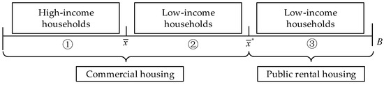
Figure 1.
Urban residential formation one: “High + Low + Low”.
(2) When , the urban residential formation is shown in Figure 2.
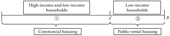
Figure 2.
Urban residential formation two: “High and Low mixing + Low”.
(3) When , the urban residential formation is shown in Figure 3.
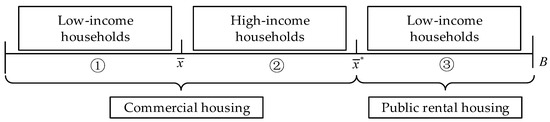
Figure 3.
Urban residential formation three: “Low + High + Low”.
Figure 1 shows the residential formation that high-income households with commercial housing are in the urban central areas, but low-income households with commercial housing are far from the urban central areas. It is consistent with the residential formation of some cities in developing country (e.g., Beijing, Shanghai in China). Because in these cities residential densities of households are higher and per capita public resources are less, high-income households prefer to live in the urban central areas to enjoy convenient traffic conditions. Figure 3 shows the residential formation that low-income households with commercial housing are in the urban central areas, but high-income households with commercial housing are far from the urban central areas. It is consistent with the residential formation of some cities in developed country (e.g., Detroit in America, Sydney in Australia). Because in these cities residential densities of households are lower and per capita public resources are higher, high-income households prefer to live in the suburbs to enjoy bigger housing space and leisure life.
It can be seen that the urban residential formation mainly depends on the relative size of and . It means the urban residential formation will change with travel cost. Let represent critical average operating speed of rail that makes urban residential formation change. When satisfies , we can obtain .
For the urban residential formation one (“High + Low + Low”), if the rail speed is raised and satisfies , the urban residential formation will still not change; if the rail speed satisfies , it will become the urban residential formation two (“High and Low mixing + Low”); if the rail speed satisfies , it will become the urban residence formation three (“Low + High + Low”). For the urban residential formation two (“High and Low mixing + Low”), if the rail speed is raised and satisfies , it will become the residence formation three (“Low + High + Low”). For the urban residence formation three (“Low + High + Low”), if the rail speed is raised, the urban residential formation will not change. It is because the increasing rail speed saves the travel time for households. High-income households will tend to move towards the suburbs to enjoy bigger floor space. As a result, the bid-rent becomes more intense in the middle of the city, and less intense in the urban central areas. In this way, low-income households will tend to move towards the city center to avoid the intense bid. Therefore, we can know that the change in average operating speed of rail will lead to the mutual transformation among urban residential formations.
2.6. Housing Equilibrium
When the housing choice of heterogeneous households reaches equilibrium, the whole urban system should meet three conditions.
(1) The housing supply equals the demand, i.e.,
where represents residential density of the household class choosing commercial housing.
Therefore, residential density of the low-income household choosing public rental housing can be calculated by
where .
When there is residential segregation between heterogeneous households choosing commercial housing, residential density of the household class choosing commercial housing can be calculated by
When there is mixed residence between heterogeneous households choosing commercial housing, we assume [10], and residential density of the household class choosing commercial housing can be calculated by
(2) All households fit inside the urban area, i.e.,
where is the number of low-income households choosing public rental housing; is the number of the household class choosing commercial housing. And , represents the total number of households in the city.
Combined Equations (42) and (46), we can obtain
Thus, urban boundary B can be calculated by
(3) The annual rental price of per unit floor space which the household class is willing to pay for commercial housing is the same at the residential demarcation separating heterogeneous households choosing the commercial housing. The land rent is equal to the agricultural land rent for at the demarcation separating urban and suburban areas, i.e.,
Combined with the housing equilibrium conditions, the equilibrium solutions of three urban residential formations are respectively given as follows.
Here, we take the urban residential formation one as an example to account for the exact meaning in detail. Equations (51) and (52) respectively stand for the annual rental price of per unit floor space which heterogeneous households are willing to pay for commercial housing in the CBD. The demarcation of heterogeneous households choosing commercial housing can be represented by the Equation (53). The demarcation between urban and suburban areas can be obtained from the Equation (54), so that the location of public rental housing can be known. Equations (53) and (54) determine the size of the residential area for heterogeneous households. All of these are related to the number of heterogeneous households, the number of public rental housing, the income level of the household and travel cost. Equations (55)–(57) indicate the equilibrium utilities of heterogeneous households choosing different housing. The first term on the right-hand side of Equation (55) denotes annual consumption quantity of non-housing goods for the low-income household choosing public rental housing. Besides this, equilibrium utility of the low-income household choosing public rental housing is related to floor space of public rental housing and demarcation of residential area. Equilibrium utility of the low-income household choosing commercial housing is related to the demarcation of heterogeneous households choosing commercial housing. While equilibrium utility of the high-income household choosing commercial housing is irrelevant to the demarcation of residential area. Similarly, when the urban residential formation changes, the results can also be found in other urban residential formations.
(1) Urban residential formation one: “High + Low + Low”.
Substituting Equations (51)–(54) into equilibrium utilities of heterogeneous households defined in Equations (13) and (20), the equilibrium utilities of heterogeneous households choosing different housing can be expressed as
(2) Urban residential formation two: “High and Low mixing + Low”.
Substituting Equations (58)–(60) into equilibrium utilities of heterogeneous households defined in Equations (13) and (20), the equilibrium utilities of heterogeneous households choosing different housing can be expressed as
(3) Urban residential formation three: “Low + High + Low”.
Substituting Equations (64)–(67) into equilibrium utilities of heterogeneous households defined in Equations (13) and (20), the equilibrium utilities of heterogeneous households choosing different housing can be expressed as
3. Numerical Study
In this section, a numerical example is provided to illustrate the properties of the proposed model and its applications. In this section, under the assumption that the number of households in the whole city is exogenously given and determined, we mainly analyze the impact of the number of public rental housing and the average operating speed of rail on the utilities of heterogeneous households. The baseline values for the parameters in this model are given in Table 1.

Table 1.
The input parameters in the numerical example.
It can easily be shown that holds for the base case. The urban residential formation for the base case is thus the “High + Low + Low” formation. In the following analysis, unless specifically stated otherwise, the input data are identical to those of the base case.
3.1. The Impact of the Number of Public Rental Housing on the Utilities of Heterogeneous Households
According to Equations (55)–(57), the impact of the number of public rental housing on the utilities of heterogeneous households can be shown as Figure 4. It means that the utilities of heterogeneous households are positively correlated with the number of public rental housing. It is because in a city with the determined population, the more public rental housing is, the fewer low-income households choosing commercial housing are. It will alleviate the bid for commercial housing for heterogeneous households, making commercial housing rental price reduce, as show in Figure 5. Thus, utilities of households choosing commercial housing will increase. Meanwhile, when the number of public rental housing is less than 1.6 × 10⁴, the utility of the low-income household choosing public rental housing is greater than that choosing commercial housing, and vice versa. It means too much public rental housing is bad for low-income households. It is because compared with low-income households choosing public rental housing, low-income households choosing commercial housing live closer to the CBD, and their travel cost is lower. When commercial housing rental price reduces to a certain extent, their total living cost (travel cost and housing cost) will be lower than households choosing public rental housing. As a result, the utility of the household choosing commercial housing grows faster. Similarly, when the average operating speed of rail changes, the results can also be found in other urban residential formations.
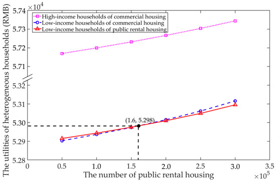
Figure 4.
The utilities of heterogeneous households with the number of public rental housing.
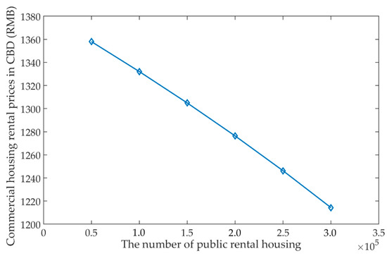
Figure 5.
Commercial housing rental prices in the central business district (CBD) with the number of public rental housing.
In order to illustrate the problem further, Figure 6 shows the total living cost and travel cost for low-income households with the same floor space but different housing with the different number of public rental housing, respectively. When the number of public rental housing exceeds 300,000, the minimum floor space of low-income households choosing commercial housing has exceeded 15 m2, so it is not considered. Figure 6a shows that the travel cost of the low-income household choosing commercial housing is far less than that choosing public rental housing. With the increasing of the number of public rental housing, the change rate of travel cost is greater when low-income households choose commercial housing. Figure 6b shows that total living cost of low-income households choosing different housing. We can know that total living cost of the low-income household choosing commercial housing is lower than that choosing public rental housing when the number of public rental housing exceeds the critical value, which is consists with our results. Anyhow, although the rental price of public rental housing is lower than commercial housing, the total living cost of the low-income household choosing public rental housing is not low when too much public rental housing was built. It is mainly caused by the remote location of public rental housing. Hence, large-scale public rental housing may be not beneficial for low-income households.
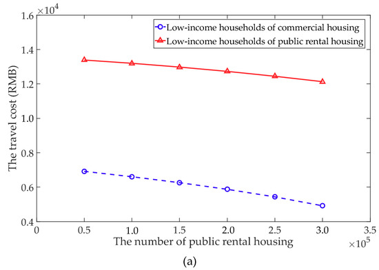
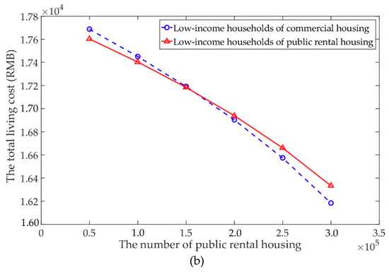
Figure 6.
(a,b) represent the travel cost and total living cost of low-income households with the number of public rental housing.
3.2. The Impact of the Rail Average Operating Speed on the Utilities of Low-Income Households Choosing Public Rental Housing
Figure 7 indicates the impact of the average operating speed of rail on the utility of the low-income household choosing public rental housing. It shows that when the average operating speed of rail changes from 40 km/h to 61 km/h, the utility of the low-income household choosing public rental housing will increase. However, when it changes from 61 km/h to 80 km/h, the utility will reduce. This is because although the increase of the rail average operating speed shortens the households’ travel time in the unit distance, it makes the boundary of the city expand outwards, which extends the households’ travel distance. Once the change of the travel distance is bigger than travel time, the total travel cost of households will increase, and the utility will reduce. Hence, the increased average operating speed of the rail may not be able to eliminate the location disadvantage of public rental housing.
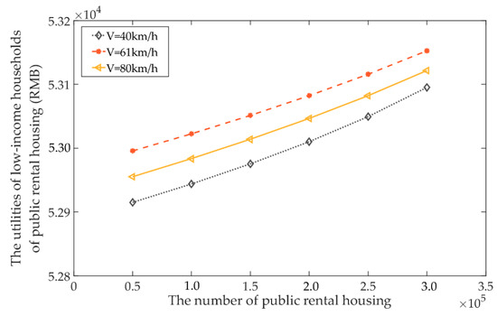
Figure 7.
The utilities of low-income households choosing public rental housing with the number of public rental housing for the rail average operating speed of 40, 61, 80 km/h.
Our results rest on the study of transportation and housing (see, e.g., Li et al. [8]; Li and Peng [10]; Li et al. [18]; Li and Guo [25]; Chen et al. [26]; Li et al. [30]), but these scholars did not analyze the public rental housing policy. Other scholars who study public rental housing policy think that the large-scale public rental housing construction is essential (see, e.g., Li et al. [3]; Shan et al. [4]; Li et al. [31]; Gan and Zhang [37]; Zheng et al. [38]); however, our results are the opposite when we consider the traffic factors. As a result, more specific and significant experiences and instructions can be referenced in this study and the model we construct could as an instruction for the joint future sustainable development of public rental housing and urban rail transit system.
4. Conclusions and Further Studies
In order to achieve stable, healthy, and sustainable development of the housing market, the public rental housing policy has been adopted by the government. As the indemnification housing policy, the public rental housing policy plays an important role in alleviating the housing pressure of low-income households and promote the sustainable development of the housing market. However, the excessive number of public rental housing will aggravate the spatial mismatch of workplace and residence, affecting the steady progress of the housing market. In order to meet the sustainable development of the housing market, we construct an equilibrium model of housing choice for heterogeneous households under the public rental housing policy. In this paper, we assume that the whole urban households are composed of high-income households and low-income households, and low-income households account for the majority of city. Once the average operating speed of rail is determined, the urban residential formation and the utilities of heterogeneous households can be determined by this equilibrium model. Based on the above study, we have found some important conclusions.
(1) We define the critical conditions for the change of urban residential formation. When the average operating speed of rail changes, it will make urban residential formation change. Low-income households will move to the CBD, and high-income households will move away from CBD.
(2) The utilities of heterogeneous households are positively correlated with the number of public rental housing, but there will be a critical value, making the utility of the low-income household choosing public rental housing lower than that choosing commercial housing. It means that ultra-limit public rental housing with a remote location is bad for low-income households.
(3) The increased average operating speed of rail does not necessarily increase the utility of the low-income household choosing public rental housing. It means that the increased speed of rail may not be able to eliminate the location disadvantage in public rental housing.
Although the proposed model in this paper provides a new avenue for exploring the effects of the public rental housing policy and the average operating speed of rail on the urban system with two income classes, some further extensions should be made.
(1) Urban population size was assumed to be fixed. However, with the advance of urbanization, a large number of migrant workers go into the cities. They are also highly concerned about public rental housing. Thus, there is a need to extend the proposed model to consider the increase of the external population.
(2) Public rental housing is assumed to be built in the suburbs. In fact, public rental housing in many cities of China is required to jointly construct with commercial housing in a certain proportion. Therefore, there is a need to extend the proposed model to consider joint construction of public rental housing and commercial housing.
Author Contributions
All authors were involved in preparing the manuscript. Conceptualization, S.Z. and H.S.; Funding acquisition, H.S.; Methodology, S.Z.; Project administration, H.S.; Resources, S.Z., H.S., T.G., and T.L.; Supervision, H.S.; Validation, S.Z.; Visualization, S.Z.; Writing–original draft, S.Z.; Writing–review & editing, S.Z., H.S., T.G., and T.L.
Funding
The work described in this paper was supported by the National Natural Science Foundation of China (71771018, 71621001).
Conflicts of Interest
The authors declare no conflict of interest.
References
- China Association of Metros. Statistics and Analysis of Urban Rail Transit in 2017. Available online: http://www.camet.org.cn/index.php?m=content&c=index&a=show&catid=18&id=13532 (accessed on 19 April 2018).
- Numbeo. Property Prices Index. Available online: https://www.numbeo.com/property-investment/rankings.jsp?title=2017 (accessed on 6 April 2018).
- Li, D.Z.; Chen, Y.C.; Chen, H.X.; Hui, E.C.M.; Guo, K. Evaluation and optimization of the financial sustainability of public rental housing projects: A case study in Nanjing, China. Sustainability 2016, 8, 330. [Google Scholar] [CrossRef]
- Shan, X.Q.; Wang, X.Q.; Ma, Y.Z.; Wu, C.M. The operation framework mechanism design of public-private partnership model of public rental housing. Adv. Inform. Sci. Serv. Sci. 2013, 5, 1210–1219. [Google Scholar]
- Ma, J.H.; Zhou, J.J.; Liu, D.D. Study on public rental housing’s maintenance in Beijing. J. Beijing Univ. Civil Eng. Architect. 2016, 32, 84–88. [Google Scholar]
- Li, X.G.; Qiu, D.C.; Li, F.; Zhen, Z. Matching analysis of the job and residence space of households in the public rental housing community in Chongqing. Geogr. Res. 2013, 32, 1457–1466. [Google Scholar]
- Ding, C.R. Urban spatial theory—Static monocentric model. Urban Stud. 2006, 13, 121–126. [Google Scholar]
- Li, Z.C.; Lam, W.H.K.; Wong, S.C.; Choi, K. Modeling the effects of integrated rail and property development on the design of rail line services in a linear monocentric city. Trans. Res. Part B 2012, 46, 710–728. [Google Scholar] [CrossRef]
- Sasaki, K. Income class, modal choice, and urban spatial structure. J. Urban Econ. 1990, 27, 322–343. [Google Scholar] [CrossRef]
- Li, Z.C.; Peng, Y.T. Modeling the effects of vehicle emission taxes on residential location choices of different-income households. Trans. Res. Part D 2016, 48, 248–266. [Google Scholar] [CrossRef]
- Jonsson, D. Sustainable Urban Development Forecasting and Appraisal. Ph.D. Thesis, KTH Royal Institute of Technology, Stockholm, Sweden, November 2003. [Google Scholar]
- Ma, X.S.; Lo, H.K. Modeling transport management and land use over time. Trans. Res. Part B 2012, 46, 687–709. [Google Scholar] [CrossRef]
- Ma, X.S.; Lo, H.K. On joint railway and housing development strategy. Trans. Res. Part B 2013, 57, 451–467. [Google Scholar] [CrossRef]
- Alonso, W. Location and Land Use: Toward a General Theory of Land Rent; Harvard University Press: Cambridge, UK, 1964. [Google Scholar]
- Kantor, Y.; Rietveld, P.; Ommeren, J.V. Towards a general theory of mixed zones: The role of congestion. J. Urban Econ. 2014, 83, 50–58. [Google Scholar] [CrossRef]
- Ng, K.F.; Lo, H.K. Optimal housing supply in a bid-rent equilibrium framework. Trans. Res. Part B 2015, 74, 62–78. [Google Scholar] [CrossRef]
- Levinson, D.M.; Xie, F.; Zhu, S. The co-evolution of land use and road networks. In Transportation and Traffic Theory 2007; Allsop, R.E., Bell, M.G.H., Heydecker, B., Eds.; Emerald Group: Bingley, UK, 2007; pp. 839–859. [Google Scholar]
- Li, T.F.; Wu, J.J.; Sun, H.J.; Gao, Z.Y. Integrated co-evolution model of land use and traffic network design. Netw. Spat. Econ. 2016, 16, 1–25. [Google Scholar] [CrossRef]
- Li, T.F.; Sun, H.J.; Wu, J.J.; Ge, Y.E. Optimal toll of new highway in the equilibrium framework of heterogeneous households’ residential location choice. Trans. Res. Part A 2017, 105, 123–137. [Google Scholar] [CrossRef]
- Muth, R.F. Cities and Housing; University of Chicago Press: Chicago, IL, USA, 1969. [Google Scholar]
- Mills, E.S. Urban Economics; Scott Foresman: Glenview, IL, USA, 1972. [Google Scholar]
- Fujita, M. Urban Economic Theory; Cambridge University Press: Cambridge, UK, 1989. [Google Scholar]
- O’Sullivan, A. Urban Economics; Irwin/McGraw-Hill: Boston, MA, USA, 2000. [Google Scholar]
- Arnott, R.J.; McMillan, D.P. A Companion to Urban Economics; Blackwell Publishing: Oxford, UK, 2006; pp. 96–108. [Google Scholar]
- Li, Z.C.; Guo, Q.W. Optimal time for implementing cordon toll pricing scheme in a monocentric city. Papers Reg. Sci. 2015, 722, 140–146. [Google Scholar] [CrossRef]
- Chen, Y.J.; Li, Z.C.; Lam, W.H.K. Modeling transit technology selection in a linear transportation corridor. J. Adv. Trans. 2015, 49, 48–72. [Google Scholar] [CrossRef]
- Gao, G.; Sun, H.J.; Wu, J.J.; Liu, X.M.; Chen, W.Y. Park-and-ride service design under a price-based tradable credits scheme in a linear monocentric city. Transp. Policy 2018, 68, 1–12. [Google Scholar] [CrossRef]
- Beckmann, M.J. Spatial equilibrium in housing market. J. Urban Econ. 1974, 1, 99–107. [Google Scholar] [CrossRef]
- Quigley, J.M. The production of housing services and the derived demand for residential energy. Rand J. Econ. 1984, 15, 555–567. [Google Scholar] [CrossRef]
- Li, Z.C.; Guo, Q.W.; Lam, W.H.K.; Wong, S.C. Transit technology investment and selection under urban population volatility: A real option perspective. Trans. Res. Part B 2015, 78, 318–340. [Google Scholar] [CrossRef]
- Li, X.; Gu, X.; Teng, Y.; Li, P. Sustainable supply model design of public rental housing—Case study of Chongqing. Front. Eng. Manag. 2014, 1, 410. [Google Scholar] [CrossRef]
- Gao, G.; Sun, H.J.; Wu, J.J.; Zhao, H. Tradable credit scheme and transit investment optimization for a two-mode traffic network. J. Adv. Trans. 2016, 50, 1616–1629. [Google Scholar] [CrossRef]
- Wheaton, W.C. On the optimal distribution of income among cities. J. Urban Econ. 1976, 3, 31–44. [Google Scholar] [CrossRef]
- Hartwick, J.; Schweizer, U.; Varaiya, P. Comparative statics of a residential economy with several classes. J. Econ. Theor. 1976, 13, 396–413. [Google Scholar] [CrossRef]
- Kwon, Y. The effect of a change in wages on welfare in a two-class monocentric city. J. Reg. Sci. 2003, 43, 63–72. [Google Scholar] [CrossRef]
- Borck, R.; Wrede, M. Political economy of commuting subsidies. J. Urban Econ. 2004, 57, 478–499. [Google Scholar] [CrossRef]
- Gan, S.Y.; Zhang, W. The exterior space design of public rental housing in mountainous city of Chongqing. Appl. Mech. Mater. 2012, 193–194, 72–76. [Google Scholar] [CrossRef]
- Zheng, C.G.; Yuan, D.X.; Yang, Q.Y.; Zhang, X.C.; Li, S.C. Management mode of super large scale project —Case as Chongqing public rental housing. Adv. Mater. Res. 2012, 594–597, 2998–3001. [Google Scholar] [CrossRef]


© 2018 by the authors. Licensee MDPI, Basel, Switzerland. This article is an open access article distributed under the terms and conditions of the Creative Commons Attribution (CC BY) license (http://creativecommons.org/licenses/by/4.0/).