Sustainability in Material Purchasing: A Multi-Objective Economic Order Quantity Model under Carbon Trading

Abstract

Sustainability in material purchasing is a growing area of research. Goods purchasing decisions strongly affect transportation path flows, vehicle consolidation, inventory levels, and related obsolescence costs. These choices have an economic impact on the supply chain, in terms of different logistic costs, and an environmental impact, in terms of the carbon emissions produced during goods transportation, storage and final recovery. In this paper, we initially analyze and compare the environmental economic policies established by the International Governments in relation to the carbon trading systems adopted. Then, we overcome a traditional single objective formulation, by developing a bi-objective lot-sizing model in which costs and emissions are kept separated and analyzed by using a Pareto frontier subject to a Cap and Trade mitigation policy. The model is useful in practice to support managers in understanding the Pareto frontier shape linked to a specific purchasing problem, defining the cost-optimal and emission-optimal solutions and identifying a sustainable quantity to purchase when a Cap and Trade mitigation policy is present. We further analyze the model behavior according to variation in market carbon price and we finally analytically demonstrate that today carbon prices are still far too low to motivate managers towards sustainable purchasing choices: there is still a gap of about 79%.

1. Introduction and Background

The international increasing concern on environmental problems stresses the need to treat inventory management and goods purchasing decisions by integrating economic, environmental and social objectives. Sustainable Purchasing [1] means taking social, environmental and financial factors into consideration in making goods procurement decisions. Several managers are now looking beyond the traditional economic parameters and are starting to make decisions based on the whole life cost, the associated risks, measures of success and impacts on society and environment. Making decisions in this way requires taking into account a number of factors linked with goods procurement:

• economic measures (such as product price, inventory costs, ordering and transportation costs),
• the entire product life cycle (i.e., [2,3,4]),
• environmental aspects (i.e., [5]),
• social aspects, as the effects on issues such as poverty eradication, inequality in the distribution of resources, labor conditions, human rights, fair-trade, as well as social consequences of air pollution due to goods transportation (i.e., [6,7]),
• use of recycled materials and product remanufacturing (i.e., [8]).

Recently, Andriolo et al. [9] claimed that the international increasing concern on sustainable purchasing policies stresses the need to treat inventory management decisions as a whole by integrating economic, environmental, and social objectives. As described by Andriolo et al. [9], an increasing number of works have been published from 2011 with the aim of incorporating sustainability criteria in the traditional Economic Order Quantity (EOQ) theory.

In the research agenda proposed by Bonney and Jaber [5], the authors briefly present an illustrative model that includes vehicle emissions cost into the traditional EOQ formulation. Hua et al. [10] extend the EOQ model to take carbon emissions into account under the cap and trade system. Analytical and numerical results are presented, and managerial insights are derived. Benjaafar et al. [11] incorporate carbon emission constraints on single and multi-stage lot-sizing models with a cost minimization objective. Four regulatory policy settings are considered, based respectively on a strict carbon cap, a tax on the amount of emissions, the cap-and-trade system and the possibility to invest in carbon offsets to mitigate carbon caps. Insights are derived from an extensive numerical study. An interactive procedure that allows the company to quickly identify the most preferred option is proposed by the authors, while Jaber et al. [2] include emissions from manufacturing processes into a two-echelon supply chain model. Arslan and Turkay [12] propose EOQ models for a number of different policies in order to show how the triple bottom line considerations of sustainability can be appended to traditional cost accounting in EOQ model. Toptal et al. [13] extend the traditional EOQ model to consider total cost and emission reduction investment under three emission regulation policies. He et al. [14] examine the production lot-sizing issues of a firm under the Cap and Trade and Carbon Tax regulations, respectively. Recently, Shu et al. [15] extend the classical EOQ model, considering carbon emissions in (re)manufacturing activities and product transportation and provide an inventory cost model with carbon constraints, while Lee et al. [16] examine a sustainable economic order quantity (S-EOQ) problem with a stochastic lead-time and multi-modal transportation options. By applying the model to various numerical scenarios, they show the effects of incorporating sustainability considerations into the traditional inventory model on operational decisions.

However, all these works apply a direct-accounting method with a single cost objective function by transforming CO₂ emissions or social effects in economic measures. Since in most cases the cost and the emission functions yield different optimal solutions, the cost trade-offs are different from the emission trade-offs ([9]). The limits of a direct accounting method when externalities need to be quantified are becoming evident in the recent literature (as also discussed by Battini et al. and Bouchery et al. [4,17]), asking for future efforts in keeping separated cost and emission functions, for instance according to a multi-objective optimisation approach.

A different way to include sustainability criteria into inventory models is proposed for the first time in the paper developed by Bouchery et al. [17], in which the authors apply a multi-objective formulation of the EOQ model abandoning the traditional approach of using a single objective function. However, in this work the authors simplify the reality by considering continuous transportation costs. Then, Andriolo et al. [18] focus the attention on the lot sizing theory when horizontal cooperation is established by supply chain partners, developing the sustainable EOQ model when two partners are cooperating in sharing transportation paths and handling units, by a multi-objective approach.

In order to follow the research agenda described by Andriolo et al. [9] and to make a step forward respect to the literature just described, the present work provides a new multi-objective Economic Order Quantity model for supporting managers in taking sustainable purchasing decisions. The model is the conceptual evolution of the previous ([4]) in which the authors provide a “sustainable EOQ model” that from an economic point of view incorporates the environmental impact of transportation and inventory holding in the total cost function, by a direct accounting approach. Here, as a second step of the research, the authors investigate the material purchasing strategy by applying a multi-objective optimization approach ([19]) in which the optimal lot-sizing decision depends on a bi-objective model with two different objective functions (costs and emissions) and transportation capacity constraints. Costs and emissions are kept separated to better reflect the effect of the lot sizing problem under analysis by also providing managers with a new decision-support tool: the Pareto frontier associated to a specific material purchasing choice. The shape of the frontier (that could be flat or steep around the cost-optimal solution) reflects the real cost and emission increments, which a manager who decides to move from a cost-optimal lot sizing solution to a more sustainable solution has to face, by better consolidating transportations.

Moreover, the Cap and Trade system approach is integrated in the multi-objective model in order to understand the impact of economic incentives (the so-called carbon allowances) on taking sustainable-oriented purchasing decisions. The Trading system used here is inspired to the current EU ETS (Emission Trading System) system (www.ec.europa.eu) and on the carbon cap evolution forecasted in the medium term. In particular, the multi-objective model here presented differs from the one developed by Bouchery et al. [17]. In this case, the transportation cost function and transportation emission function are modelled according to their real nature: piecewise convex function of the ordering levels with discontinuities at the cost breaks (the transportation vehicles’ saturation points), unlike the traditional model where the total cost is convex over the entire range of ordering levels ([17]). This formulation is essential to better understand and quantify the benefit of transportation consolidation when deciding goods purchasing lot sizes. Finally, the model behavior is investigated according to variation in market carbon price, analytically demonstrating that current carbon prices are still far too low to motivate managers towards sustainable purchasing choices: there is still a gap of about 79%.

This paper is organised as follows. In Section 2 we present a brief overview of the Cap and Trade mitigation policy and the effects of the carbon trading market. In Section 3 the multi-objective EOQ model formulation is presented and the interactive decision making approach is explained. A parametric analysis is provided in Section 4 to better discuss the effect of Cap and Trade mechanism on buyers’ decisions, according to variation in the carbon market price. Finally, Section 5 discusses the conclusions.

2. Cap-and-Trade System and EU Carbon Price Value Trend

Cap-and-trade (C&T) and carbon tax are two emission regulations widely used to curb the carbon emissions generated from firms and air-transportations in EU, US States, and New Zealand ([20]). Reference [21] argues that C&T has a number of important advantages compared to carbon tax, such as political feasibility, cost effectiveness, broad participation, equity in the international context, and control on the cumulative quantity of emissions.

The Emission Trading System (ETS) is a cost-effective way of the European Union’s policy to combat climate change and to reduce industrial greenhouse gas emissions (GHG). It has been launched in 2005 and it works on the “cap and trade” principle ([2]): a cap is set on the total amount of a certain GHG that can be emitted by factories, power plants, and other installations. The cap is reduced over time, in this way the total emissions decrease. The target for 2020 is a reduction of 20% of GHG emissions compared to 1990 levels. The EU ETS regards, in particular, power plants, a wide range of energy-intensive industry sectors and operators of flights to and from the EU, Iceland, Liechtenstein, and Norway. The companies involved into this system sell or buy emission allowances, which they can trade with one another as needed. Each allowance corresponds to the right to emit 1 tonne of CO₂. Businesses must report their EU ETS emissions every year and provide enough allowances to cover them by 30 April of the following year. If a business does not surrender enough allowances to cover its emissions, it must buy allowances to make up the shortfall; its name is published, and has to pay a fine for each excess tonne of greenhouse gas emitted (www.ec.europa.eu). This policy, by putting a price on carbon, implies some interesting consequences: each tonne of emissions saved has a financial and commercial value and a sufficiently high carbon price can promote investment in clean, low-carbon technologies. The price of carbon allowances (the so-called carbon price) is determined by supply and demand according to a market-oriented mechanism. During the first phase of EU ETS (2005–2007), the price of allowances increased up to a peak level of about €30/tCO2e in April 2006 (www.publications.parliament.uk). Nevertheless, the excess of allowances led to a trading price of €0.10 in September 2007. The estimated needs were excessive; in this way, the allowances price fell to zero (www.ec.europa.eu). During the Phase II (2008–2012) the carbon price increased to over €20/tCO2e in the first half of 2008, but the 2012 closed with a price of around 6.67 €/tCO2e. One main reasons for this fall in prices was that the economic downturn led to a reduced output in energy-intensive sectors; therefore, less abatement has been required to respect the cap and the market has been oversupplied with permits, leading to the downfall of the price. For Phase III (2013–2020) the European Commission has proposed some changes that during the first three quarters of 2015 conducted the allowances price trend to rise. The allowances average price from the third quarter of 2015 until the first quarter of 2017 was between €7.90 (EEX-DE platform) and €7.92 (EU t-CAP platform). From March 2017 a positive trend is present and at the end of April 2018 the carbon price was around 13.4 €/tCO2e and then it grew again for the entire month of August 2018 to about 21 €/tCO2e (on 27 August 2018): this trend is considered from some major analysts an indicator for a long-term growing trend (www.gse.it).

The International Emissions Trading Association (IETA, www.ieta.org) describes some of the emissions trading advantages:

• Cap-and-trade is designed to fulfil an environmental outcome, in that the cap must be met
• This trading scheme will deliver its environmental objective at lowest cost to the economy.
• It can be fundamental for setting a global agreement to reduce emissions: national trading systems can be linked with other similar systems, driving to a global carbon market.
• Cap-and-Trade offers to business both compliance and policy flexibility, it delivers an economic incentive to the companies able to innovate and find more effective ways of reducing emissions.
• Cap-and-trade has proven effectiveness: for example, in the US acid rain program it quickly reduced pollution levels at a lower cost than expected.

3. Theoretical Formulation

The mathematical formulation that follows tries to capture economic and environmental trade-offs in material purchasing lot sizing. It is considered the single-product replenishment problem and applied a bi-objective optimization approach by modelling the EOQ problem for incoming goods to be purchased by a company, in accordance with two distinctive objective functions: the total annual cost function and the total emission cost function. It is supposed that the product demand is deterministic, the product price is exogenous and the buyer decides only the order size.

First, we introduce the notations used in the model as follows:

Indices

$i$ container/vehicle type

$j$ transportation mode

Decision Variables and Cost Functions

$Q$ decision variable [units/purchasing order]

$C\left(Q\right)$ total average annual cost of replenishment [€/year]

$E\left(Q\right)$ total annual emission generated by the replenishment [CO2e/year]

$Q_c^{\ast }$ optimal order quantity for the cost function [units/purchasing order]

$Q_e^{\ast }$ optimal order quantity for the emission function [units/purchasing order]

Input Parameters

$D$ annual demand [units/year]

$p$ unit purchase cost [€/unit]

$p’$ unitary scrap price [€/unit]

$b$ space occupied by a product unit with sale packaging [m³/unit]

$a$ weight of a unit stored in the warehouse [ton/unit]

$O$ fixed ordering cost per order [€/order]

$h$ holding cost [€/unit]

$\beta$ average inventory obsolescence annual rate [%]

$y$ full load-vehicle/container capacity [units or m³]

$v$ average freight vehicle speed [km/year]

$d_j$ distance travelled by transportation mode $j$[km]

$c_{f,j}$ fixed transportation cost coefficient for transportation mode $j$ [€/km]

$c_{v,j}$ variable transportation cost coefficient for transportation mode $j$ [€/km m³]

$c_{ef,j}$ fixed transportation emission coefficient for transportation mode $j$ [kgCO2e/km]

$c_{ev,j}$ variable transportation emission coefficient for transportation mode $j$ [kgCO2e/km m³]

$c_{eh}$ warehouse emission coefficient [kgCO2e/m³]

$c_{eo}$ waste collection and recycling emission coefficient [kgCO2e/ton]

$n_i$ number of full load-vehicle/container $i$ [units]

$y_i$ full load-vehicle/container $i$ capacity [units]

$k$ range of order quantity $Q_s$ between the two discontinuity points $D{P}_k$ and $D{P}_{k+1}$

$D{P}_k$ Discontinuity Point for range $k$, defined as ${\sum }_i{n}_i·y_i$

$S_j$ freight vehicle $j$ utilization ratio in %

$C$ value of carbon price quoted in the market [€/tCO2e]

$cap$ carbon cap according to a cap and trade system [tCO2e]f

cap% emission reduction by reaching the cap value respect to the maximum emission value

$\mathsf{\Delta }{E}_{cap}$ emission reduction by reaching the cap value [tCO2e]

$\mathsf{\Delta }{C}_{cap}$ cost increment by reaching the cap value [€]

Unlike prior models already discussed in Section 1, transportation costs are here considered explicitly and modeled according to their true discontinuity nature.

Let us introduce the first objective function $f_1\left(Q\right)$ that quantifies the average annual cost of replenishment and it is expressed as follows:

$$f_1\left(Q\right)=C\left(Q\right)=p·D+C_o\left(Q\right)+C_h\left(Q\right)+C_{obs}\left(Q\right)+C_t\left(Q\right)$$

(1)

In detail, the terms included in this formulation are defined as follows (from [4]). The ordering cost $C_o\left(Q\right)$, associated only to the buyer fixed cost of processing the order, and the holding cost $C_h\left(Q\right)$ are calculated according to the traditional models:

$$C_o\left(Q\right)=\frac{D}{Q}·O$$

(2)

Holding cost now considers both the traditional holding cost of carrying inventory in the warehouse and the cost associated to hold inventory during the transportation activity that is not as function of $Q$, as expressed by the following formula (derived from [22]):

$$C_h\left(Q\right)=\frac{Q}{2}·h+Q·\frac{d}{v}·\frac{D}{Q}·h$$

(3)

where $v$ is the freight vehicle speed expressed in km/year.

To make the application of this formulation less time-consuming, a simple but plausible formulation for obsolescence cost $C_{obs}\left(Q\right)$ is here applied:

$$C_{obs}\left(Q\right)=\frac{Q}{2}·\left(p-p^{\prime }\right)·\beta$$

(4)

An obsolete event comes from a specific cause (i.e., a change in the product design or in product technical specification) and makes immediately unusable the inventory on hand. We here apply the obsolescence annual risk rate $\beta$ according to [4]. At the end of each year, the remaining stocks are sold by the buyer to a specific waste treatment company for disposal at the unitary scrap price $p’$, lower than $p$. In some cases, $p’$ could also become negative, for example if the owner has to pay the waste treatment company for the disposal service.

Due to the relevance of transportation cost $C_t\left(Q\right)$ on the optimization of the order quantity [23], its formulation includes both fixed and variable costs and it presents Discontinuity Points $D{P}_k$ when the vehicle capacity is saturated. Thus, we express the transportation costs with the sum of a fixed portion (expressed in €/km since it does not increase with the order quantity but only with the travelled distance) and a variable portion, which depends on the quantity transported and on the vehicle saturation.

The vehicle saturation $S_j$ depends on the quantity transported, on vehicle capacity $y_i$ and on the number of vehicles used in the order cycle $n_i$:

$$S_j=\frac{Q}{{\sum }_i{n}_i·y_i}$$

(5)

under the following constraint:

$${\sum }_i{n}_i·y_i\ge Q$$

(6)

As discussed in previous studies [4,23], the transportation cost is not a continuous function and it cannot be differentiated during the whole interval. Moreover, the value $n$ depends on the number of different vehicle types used in the transportation (for example different containers with different capacities). In practice, in a global supply chain scenario, more types of vehicle are available with different capacities and different costs. Hence, it is necessary to accurately evaluate all the discontinuity points and ranges between them and apply a step-by-step approach, as already adopted in literature. To simplify the problem, when $D{P}_k$ is the Discontinuity Point $k$, obtained after the accurate evaluation of all capacity saturation ranges of different kinds of container i that are applied in the same purchasing cycle, we can assert that, in general:

$$S_j=\frac{Q}{{\sum }_i{n}_i·y_i}=\frac{Q}{D{P}_k}$$

(7)

and, then, express the transportation cost $C_t\left(Q\right)$ for each kind of transportation mode $j$ used, as follows [4]:

$$C_t{}_j\left(Q,d_j,S_j\right)=\left(c_{f,j}·d_j·{\sum }_i{n}_i+c_{v,j}·d_j·D{P}_k\right)·\frac{D}{Q}$$

(8)

Concluding, the first function to optimize is expressed as follows (considering the whole mix of transportation modes used in the material supply from vendor to buyer):

$$f_1\left(Q\right)=C\left(Q\right)=p·D+\frac{D}{Q}·O+\frac{Q}{2}·h+\frac{d}{v}·D·h+\frac{Q}{2}·\left(p-p^{\prime }\right)·\beta +{\sum }_j\left(c_{f,j}·d_j·{\sum }_i{n}_i+c_{v,j}·d_j·D{P}_k\right)·\frac{D}{Q}$$

(9)

The second objective function $f_2\left(Q\right)$ is the average total quantity of emissions generated during the annual purchasing activity and it can be expressed by the sum of the emissions generated in the following three steps: material order transportation, warehousing, and waste collection and treatment of the obsolete items. Thus, by an environmental point of view, only three terms must be considered and homogeneously expressed in tons of CO2e:

$$f_2\left(Q\right)=E\left(Q\right)=E_h\left(Q\right)+E_{obs}\left(Q\right)+E_t\left(Q\right)$$

(10)

The first term computes the average quantity of equivalent carbon emissions generated by warehousing during the time unit of one year:

$$E_h\left(Q\right)=c_{eh}·\frac{Q}{2}·b$$

(11)

Here, $c_{eh}$ is the average emission cost coefficient of a warehouse expressed in € per cube meter of warehouse space occupied by inventory (this coefficient differs in case we use or not a temperature controlled warehouse), and $b$ measures the cube meters occupied by a product unit stored in the warehouse (considering also packaging materials).

The inventory stored in the warehouse presents a risk of obsolescence at the end of the year, expressed by the obsolescence annual risk rate $\beta$. Obsolescence goods at the end of the year are sold by the buyer to a specific waste treatment company for recycling at the disposal price $p’$, lower then $p$. Anyway, in this case we only consider the emissions generated during the waste collection and treatment process. Therefore:

$$E_{obs}\left(Q\right)=\frac{Q}{2}·\beta ·a·c_{eo}$$

(12)

where $c_{eo}$ is the carbon emission cost coefficient for obsolete inventory waste collection and recycling, expressed in €/ton and $a$ is the weight of an obsolete unit stored in the warehouse in tons/unit. Finally, due to the reasons described above and to the discontinuity nature of the transportation cost function, also the emission function linked to the transportation activity is described by a discontinuous function, as follows:

$$E_t{}_j\left(Q,d_j,S_j\right)=(c_{ef,j}·d_j·{\sum }_i{n}_i+c_{ev,j}·d_j·D{P}_k)·\frac{D}{Q}$$

(13)

Thus, the second objective function to optimize is finally expressed as follows (considering the whole mix of transportation modes used in the material supply from vendor to buyer):

$$f_2\left(Q\right)=E\left(Q\right)=c_{eh}·\frac{Q}{2}·b+\frac{Q}{2}·\beta ·a·c_{eo}+{\sum }_j\left(c_{ef,j}·d_j·{\sum }_i{n}_i+c_{ev,j}·d_j·D{P}_k\right)·\frac{D}{Q}$$

(14)

According to a generic Pareto design optimization problem [19] involving the two conflicting objective functions introduced above, it can be concisely stated:

$$Minimize\left\{f_1\left(Q\right),f_2\left(Q\right)\right\}$$

(15)

A Pareto-optimal solution is also defined “Pareto-efficient solution”, and the set of all efficient points is called the Pareto Frontier. It is generally impossible to come up with an analytical expression of the Pareto Frontier; however, a basic requirement for Pareto optimality is expressed in the following:

“$Q^{\ast }$ is a Pareto-optimal solution to the problem posed by Equations (9) and (14), if there does not exist any other design $Q$ such that $f_1\left(Q\right)\le f_1\left(Q^{\ast }\right)$ and $f_2\left(Q\right)\le f_2\left(Q^{\ast }\right)$ simultaneously.”

The number of Pareto-efficient solutions $Q^{\ast }$ can be quite large, and it is yet necessary to select the best compromise design(s) among them. Thus, a sustainable purchasing choice normally increases $f_1\left(Q\right)$, while decreases $f_2\left(Q\right)$, since the two objective functions are competitive in nature.

If $Q{Q}_c^{\ast }$ is the single optimal solution of the objective function $f_1\left(Q\right)$ and $Q{Q}_e^{\ast }$ is the single optimal solution of $f_2\left(Q\right)$, we can call $EF$ the Efficient Frontier of the lot sizing problem here proposed and $E{F}^c$ its image in the criterion space, then:

$$EF=\lfloor Q{Q}_c^{\ast },Q{Q}_e^{\ast }\rfloor$$

(16)

$EF{Q}_{+}^c$ is convex and there exists $Q_{min}<Q_{max}$ such that $Q^{\ast }\in \left[Q_{min},Q_{max}\right]$.

As a consequence, the shape of the $EF$ strongly affects the possibility to move from a cost-optimal solution to an emission-optimal one.

We can now define the following three measures, all related to the $EF$ shape:

$$\mathsf{\Delta }Q=Q_{max}-Q_{min}=\left|Q{Q}_c^{\ast }-Q{Q}_e^{\ast }\right|$$

(17)

$$\mathsf{\Delta }C=f_1\left(Q_{max}\right)-f_1\left(Q_{min}\right)$$

(18)

$$\mathsf{\Delta }E=f_2\left(Q_{max}\right)-f_2\left(Q_{min}\right)$$

(19)

The first one expresses by a quantitative point of view the extension of the efficient frontier curve in the space, that is, the distance between the emission-optimal solution and the cost-optimal solution in term of purchasing units. By computing the rate $\mathsf{\Delta }C/\mathsf{\Delta }E$ we can express the expected marginal increment in annual logistic cost per ton CO2e, in order to move towards an emission optimal solution instead of a cost optimal solution. The solution of the multi-objective problem under consideration can be achieved using the concept of indifference band [24]. An indifferent band is the area on the Cartesian coordinate plane where the feasible solutions are all equally desirable to the decision maker. Between any two solutions in the indifference curve there is a trade-off, so that a decrement in the value of one objective function $f_i$ inevitably determines an increment in the other objective function $f_j$.

When a carbon cap is set according to a Cap and Trade regulatory policy, a company can decide to reduce the total emissions below the cap in order to respect the governmental constraint; on the contrary, the company has to buy carbon allowances on the carbon market.

By a traditional cost-oriented optimization approach, a company prefers to apply a cost-optimal solution in order to minimize the total annual purchasing cost, so that the costs are at minimum but, consequently, the emissions are maximized ($Q{Q}_c^{\ast }$).

In order to reduce the total annual emissions below the cap value, the company has to move in the Pareto Frontier from right to left until it is possible to define a transportation quantity that is applicable as a purchasing lot size.

In doing this, the company will inevitably increase its annual costs. We here define this marginal increment in total annual costs as the Marginal Logistic Cost ($MLC$), defined as follows:

$$MLC=\frac{\mathsf{\Delta }{C}_{cap}}{\mathsf{\Delta }{E}_{cap}}$$

(20)

The concept of $MLC$ is shown in Figure 1.

The $MLC$ value varies according to the different shapes of the Pareto Frontier, which in some industrial sectors could be steep or on the contrary more flat. When a carbon cap is coupled with a carbon allowance in a cap and trade system, the market carbon price $C$ represents the allowance that helps the company to fit and go under the defined carbon limit (the cap).

By introducing the parameter φ defined as follows:

$$\phi =\frac{MLC}{C}$$

(21)

Three different situations could be identified in practice:

• $\phi >1$: the $MLC$ is major than the carbon price and the company has two options:
  • buy carbon allowances in the carbon market instead of investing in reducing emissions by transportation consolidation
  • autonomously sustain an extra cost in order to reduce its emissions under the cap value equal to $MLC-C$
• $0<\phi \le 1$: the $MLC$ is lower or at least equal to $C$ and the company could earn by the reduction of emissions an extra saving equal to $C-MLC$. For this reason, the company is fully economically supported and the company decision maker is motivated in increasing the purchasing quantity of incoming materials while saturating vehicles.
• There is no feasible solution to better consolidate transportation since the cost-optimal solution is equal to the emission-optimal solution: the company could only change the supplier or the transportation modality.

In the next paragraph a numerical application of the model with a parametrical analysis is reported in order to understand how the Pareto Frontier shape specifically built for each industrial case could affect the value of the parameter $\phi$ and the consequent emission reduction. The proposed bi-objective model does not aim at finding a single optimal solution at once. The problem could be solved only by an interactive approach during the decision-making [25]. The decision makers (as managers and buyers) by yielding all of the potentially optimal solutions and by understanding the shape of the Pareto Frontier in each specific case, can understand the trade-offs between extra-logistic costs and economic incentives (carbon allowances) and finally define how to improve their purchasing strategy.

4. Parametric Analysis and Discussion

In this section we present a parametric analysis, directly inspired by real industrial cases, to illustrate the above analytical model and provide some observations of the Cap and Trade system applied to the material purchasing and transportation setting.

Let us consider a set of different goods purchased and transported inside logistic load units (i.e., stock keeping unit, box, etc.), each of them with a different weight and volume. The product purchasing price changes in order to provide results suitable for a wide range of real situations. The products considered in the following example can be easily assimilated to different industrial sectors (from small electrical equipment, cellular phones, computers to fashion items and metal parts etc.). The buyer’s company is located in the North-East part of Italy and closed to intermodal terminals, while the vendor is located overseas (e.g., in Hong Kong). Transportations are made by adopting a rail-ship intermodal transport with only a final short handling by truck.

Constant input data and fixed transportation costs values reported in

Table 1. Constant Input data.

Constant Input Data	Value	Constant Input Data	Value
$D$	40,000	$c_{v,road}$[€/km∙m3]	0.01
$O$[€/order]	400	$c_{f,rail}$[€/km]	0.6
$d$[km on road]	100	$c_{v,rail}$[€/km∙m3]	0.007
$d$[km by train]	500	$c_{f,ship}$[€/km]	0.48
$d$[km by ship]	14,000	$c_{v,ship}$[€/km∙m3]	0.003
Inner volume container1 [m3]	33.2	$c_{eh}$[kgCO2e/m3∙year]	24
Load Capacity container1 [tons]	21.75	$c_{eo}$[kgCO2e/ton]	77.004
Inner volume container2 [m3]	67.2	$c_{ef,road}$[kgCO2e/km]	2.20017
Load Capacity container2 [tons]	26.70	$c_{ev,road}$[kgCO2e/ton∙km]	0.154398
$v_{road}$[km/year]	525,600	$c_{ef,rail}$[kgCO2e/km]	1.28017
$v_{rail}$[km/year]	788,400	$c_{ev,rail}$[kgCO2e/ton∙km]	0.0392892
$v_{ship}$[km/year]	219,000	$c_{ef,ship}$[kgCO2e/km]	0.06443
$c_{f,road}$[€/km]	0.8	$c_{ev,ship}$[kgCO2e/ton∙km]	0.0088875
$\rho$[kg/m3]	300	$\beta$[%]	15

are derived from [4], while carbon footprint coefficients are calculated using the Ecoinvent database in SimaPro Software (www.simapro.co.uk). The cost and emission functions reported in Formulas (9) and (14) are computed in relation to the set of discontinuity points $D{P}_i$ identified according to the different handling units used in the purchasing network (container 1: ISO 20 feet and container 2: ISO 40 feet). The input parameters subject to variations are reported in

Table 2. Variable Input data.

Variable Input Data	Set of Values
$p$ [€/unit]	[1; 10; 20; 40; 70; 110; 160; 220; 290; 370]
$a$ [kg/unit]	[0.5; 1; 5; 10; 20]

.

Table 3. Dependent Variables.

Dependent Variables	Relation with Variable Input Data
$b$ [m3/unit]	$a/\left(\rho ·1000\right)$
$p’$ [€/unit]	0.5∙$p$
$h$ [€/unit]	0.25∙$p$
$y_1$ [units/container1]	Min (Inner volume container1/$b$; Load Capacity container1/$a$)
$y_2$ [units/container2]	Min (Inner volume container2/$b$; Load Capacity container2/$a$)

lists all the dependent variables in the model, with relation to the input data. The saturation of the two types of containers can be achieved by volume or by weight, depending on the characteristics of the product (see Table 3). From Table 1, it can be noticed that the Apparent Density $\rho$ has been introduced and in the present numerical application it is fixed to 300 kg/m³, in order to generate plausible situations for the type of products under consideration. The risk of obsolescence of the inventory is supposed fixed and equal to $\beta$ = 0.15.

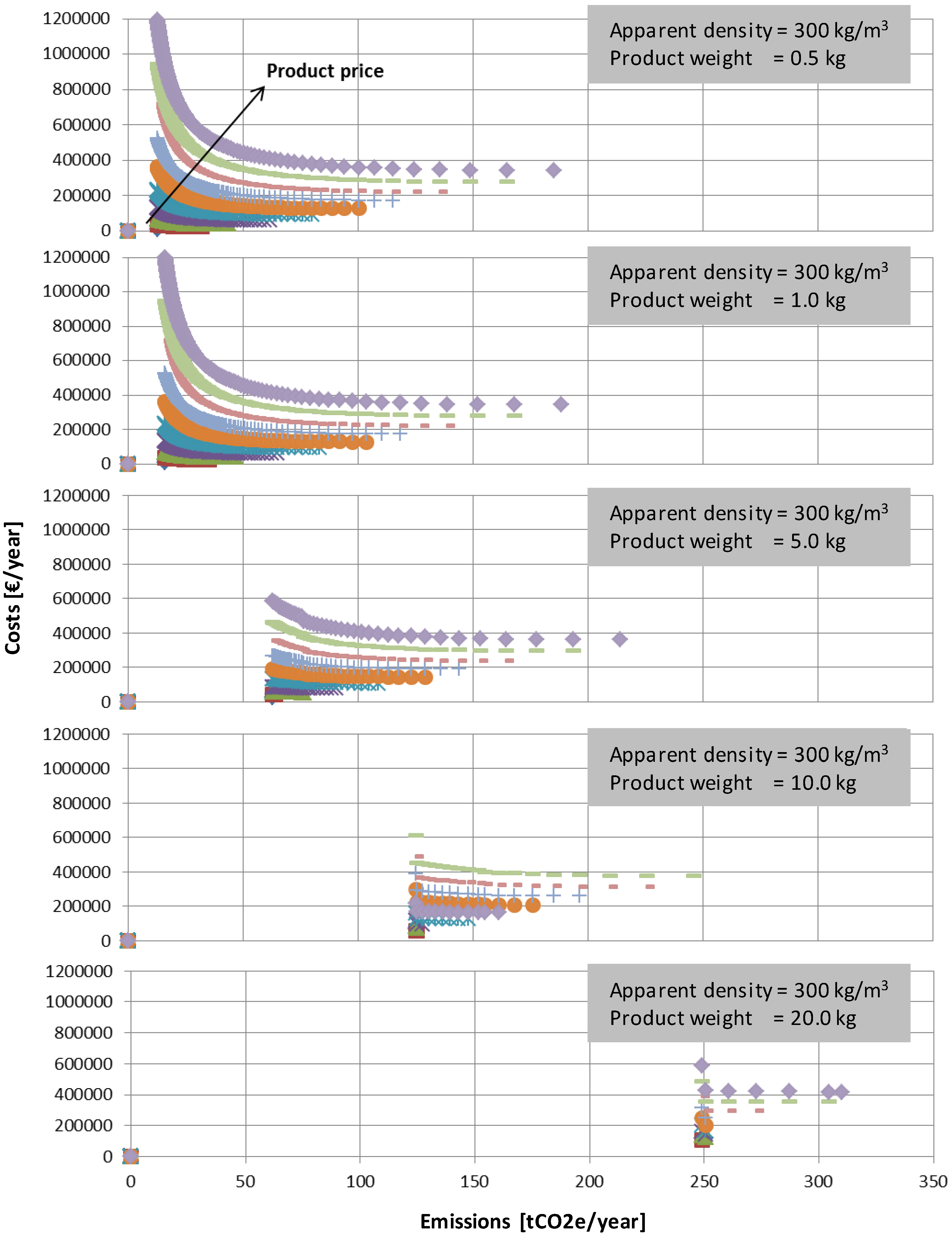
Figure 2 shows the trend of the Pareto Frontiers for the 5 different values of product weight reported in Table 2. Note that the scales are the same for all the graphs, in order to facilitate a visual comparison. At a first glance, we immediately notice that as the product weight increases, the width of the frontiers decreases, then the number of Pareto optimal solutions belonging to the Frontier decreases. Moreover, the frontiers move from lower to higher values of the total emissions, but at the same time, the total annual costs decrease. Consequently, they move towards the right lower part of the Cartesian plane. At equal weight instead, as the product price increases, the efficient solutions move towards higher values for both costs and emissions.

By comparing the different Pareto Frontier shapes in Figure 2 we can summarize the following:

• each material purchasing decision has a specific Pareto Frontier associated, which is capable to drive the decision maker to the final choice according to an interactive approach;
• the more the frontier is large and flat around the cost-optimal solution, the more possibilities exist to increase the purchasing lot sizing quantity with a consistent reduction in emission and a limited increment in total costs;
• when the product weight is low and the product purchasing price is high, the Frontier is large and flat around the cost-optimal solution, leaving possibilities to managers to increase the purchasing lot size, saturate vehicles and reduce emissions;
• when the product weight is higher and product price is lower, $\mathsf{\Delta }C$ and $\mathsf{\Delta }E$ are reduced, and the frontier is shorter and constituted only by some few points. This happens since the vehicles are saturated faster;
• the trend of the outputs in relation to the price $p$ is also evident: for the same value of the product weight, lower values of the product price $p$ determine lower values of $\mathsf{\Delta }C$ and $\mathsf{\Delta }E$; when it increases, also the gap between the two optimal lot sizing solution $Q{Q}_c^{\ast }$ and $Q{Q}_e^{\ast }$ increases and, thus, both $\mathsf{\Delta }C$ and $\mathsf{\Delta }E$ become higher.

Finally, a sensitivity analysis of the parameter $\phi$ introduced in the previous paragraph is performed, according to variations in product price (from 5 to 1000 €/item) and product weight (from 0.5 to 5 kg/item), in order to understand the incidence of the marginal logistic cost with respect to the market carbon price applied under a Cap and Trade approach. The results are reported in Figure 3 and Figure 4. 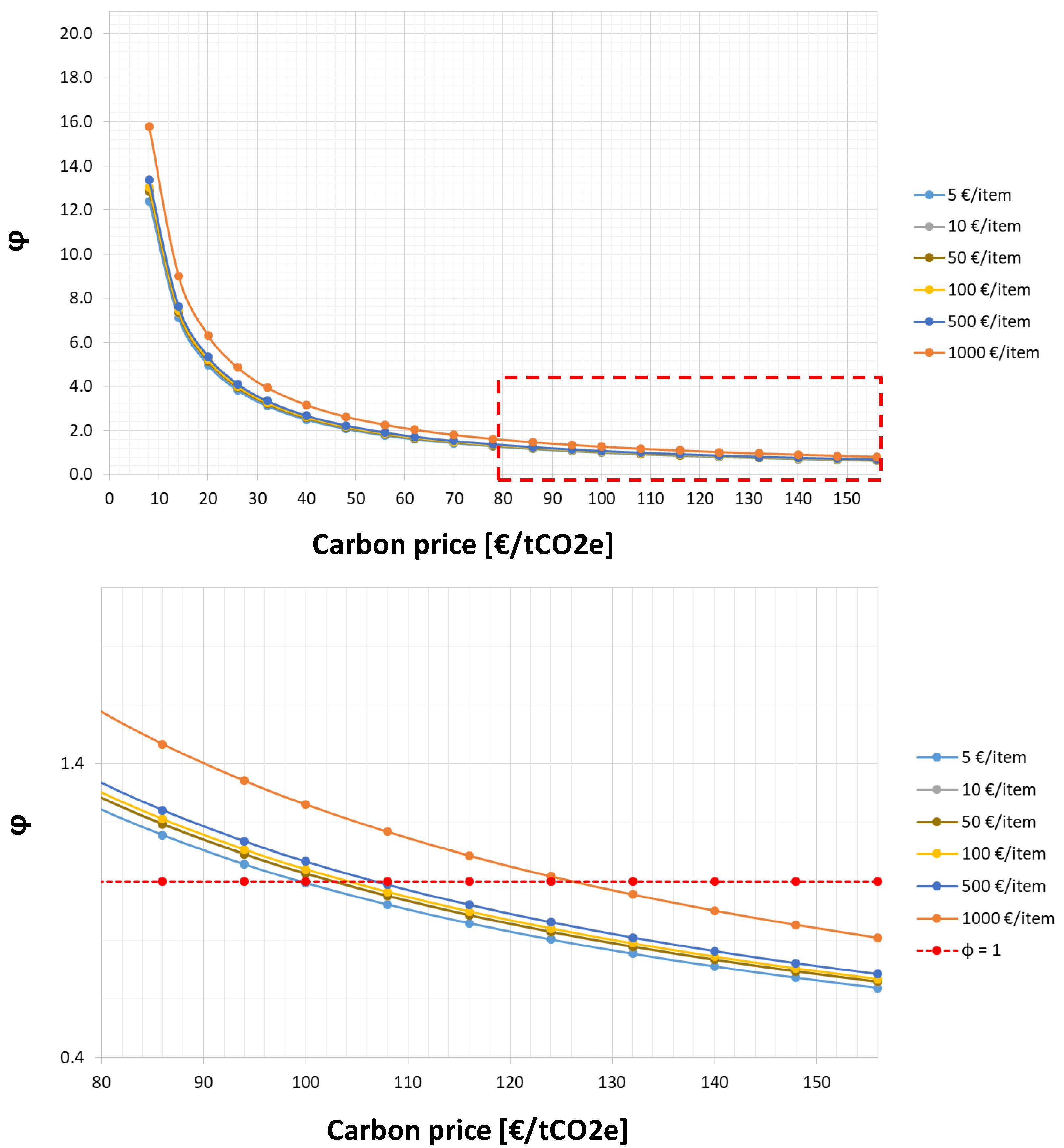Figure 3 shows the trend of the parameter φ in relation to the product price. In the case illustrated in the Figure 3, the product weight is set at 0.5 kg/item and it is required an emission reduction to reach the cap of 10% (cap%) It is shown that the higher the product price, the higher is the φ value. This means that for a higher product price, larger extra costs and profit sacrifices are required to the company in order to reduce its annual emissions below the cap and to perform an efficient transportation vehicle saturation. Therefore, more expensive products reach φ values equal or lower than 1 for higher carbon price values: the φ value starts to be equal to 1 only with a carbon price major than 100 €/tCO2e when the product price is equal to 5 €/item. By considering the current carbon price of 21 €/tCO2e (28 August 2018), the φ value is close to 5 when the product price is 5 €/item, which means that the company needs to invest 5 times the carbon allowance value in order to reduce emissions of 1 tCO2e.

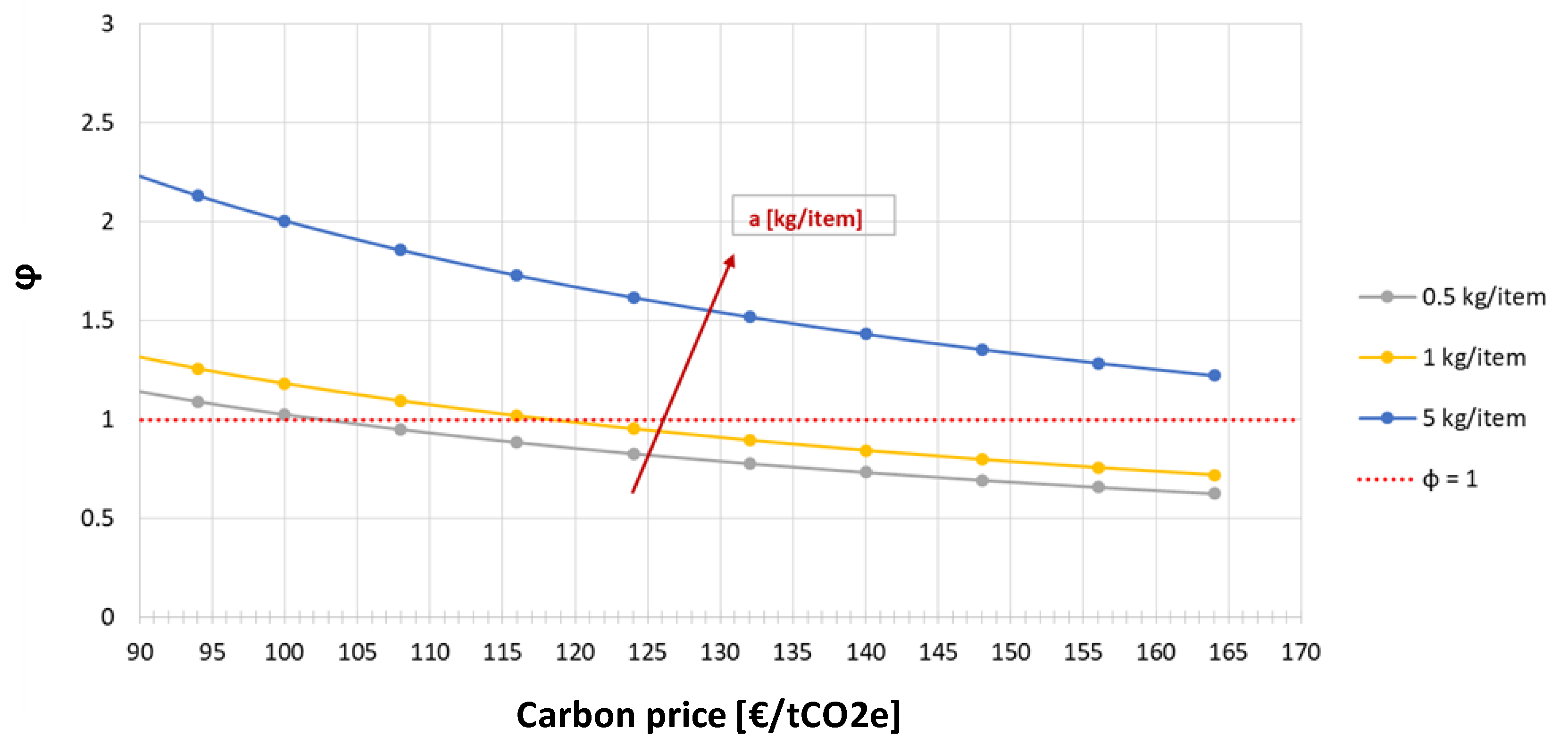
The same situation is also evident in Figure 4, showing the trend of the parameter φ in relation to the product weight. In the case illustrated the product price is set at 50 €/item and it is required also in this case an emission reduction to reach the cap of 10% (cap%) for an item purchasing. It is shown that the higher the product weight, the higher is the φ value. This means that for a higher product weight, bigger extra costs are required to the company in order to reduce its annual emissions under the cap. Therefore, heavier products reach φ values equal or lower than 1 for higher carbon price values, and always with a carbon price major than 100 €/tCO2e. This means that with the current carbon price values (21 €/tCO2e in the ETS system in 27 August 2018) significant extra costs and profit sacrifices are necessary for the company in order to reduce its annual emissions under the cap and there is still a gap of 79% in order to reach a φ value equal to 1.

Thus, a cap-and-trade system if applied to the material purchasing and transportation sector should be carefully adapted to each industrial sector and should also provide a higher value of the carbon price value in order to really incentive companies towards sustainable choices. We demonstrate for the first time, by a mathematical point of view, that current carbon price values are still far too low to motivate managers towards sustainable purchasing choices.

However, managers highly oriented to sustainable choices could always decide to reduce emissions instead of buying carbon allowances by accepting to increase the total purchasing cost and reducing their profit margins.

5. Conclusions

The paper develops a multi-objective EOQ model that considers a typical global supply-chain purchasing problem with long-distance freight transportation, but it could be also applied to a domestic transportation case. Total purchasing costs and total CO₂ equivalent emissions are taken into account to build the Pareto Frontier as a tool to support managers’ decision making in an interactive way. The model is applied to a simple set of numerical scenarios, where a number of input data are fixed and inspired to a real case, while other product features (weight and product purchase price) assume various values. The parametric analysis here developed permits to analyze the different shapes of the Pareto Frontiers according to the variations in these key parameters. Moreover, the model introduces for the first time the parameter φ in order to better support managers in understanding the economical convenience in reducing carbon emissions by taking a sustainable purchasing choice. The parameter is the rate between the marginal increment in total annual costs, the Marginal Logistic Cost ($MLC$), and the market carbon price $C$, that represents the allowance that helps the company to fit and go under the defined carbon limit (the carbon cap). Only with φ < 1, the company is economically motivated to reduce emissions by consolidating transportations and increasing purchasing lot size; otherwise, until the φ parameter is higher than 1, the company needs to autonomously sustain an extra cost in order to reduce its emissions under the cap value.

The graphical results provided in Figure 3 and Figure 4 permit to summarize the following main conclusions:

(a)

A bi-objective approach to material purchasing overcomes the limits of a direct cost accounting approach in which emissions are transformed in costs and only a single objective function is considered, as previously highlighted also in [4,9].

(b)

By a practical point of view, the analysis of the Pareto frontier is useful to address managers towards the correct comprehension of the sustainable purchasing problem, by identifying the cost-optimal and the emission-optimal solutions, while having an immediate comprehensive visualisation of Pareto frontier shape (Figure 1).

(c)

The purchasing manager can be driven to decide the material purchasing quantity to order when a cap and trade mitigation policy is present, with an immediate comprehension of the effects of his/her choice in terms of emissions and costs (Figure 1).

(d)

The Carbon Trading systems currently applied by Governments in order to mitigate the emission production in some critical sectors, is a promising tool to be applied also in the field of freight transportation and material purchasing when ship/train/road transportation modes are considered.

(e)

In this paper, we analytically demonstrate that the current carbon prices (i.e., 21 €/tCO2e at the end of August 2018 in the ETS trading system) are still too low to sustain and economically motivate a feasible extension of the cap-and-trade policy to the freight transportation sector and to the sustainable purchasing problem under analysis. In fact, Figure 3 and Figure 4 show that, by considering the current carbon price of 21 €/tCO2e (28 August 2018), there is still a gap of 79% in order to reach a φ value equal to 1.

(f)

The current positive trend in worldwide carbon price values (especially in Australia and Japan) is quite encouraging: if the carbon price will reach in the near future the threshold of 100 €/tCO2e, the cap and trade mechanism will start acting as an economic incentive for company managers and buyers towards more sustainable purchasing choices.

(g)

However, even without the presence of effective carbon mitigation policies, a purchasing manager can always decide to apply a sustainable purchasing quantity to better consolidate transportation, by accepting a profit sacrifice in order to be more sustainable. The higher the profit margin of the item purchased is and the lower the sacrifice asked to the purchasing company will be in order to be more sustainable.