The Impact of Micro-Level Influencing Factors on Home Value: A Housing Price-Rent Comparison

Abstract

The housing sales market in China has flourished and gained considerable interest, while the housing rental market has lagged behind and been ignored over the past two decades. With the acceleration of urbanization, the housing rental demand is rising rapidly. Exploring and comparing the influencing factors on housing sale prices and rental prices has significance for sustainable urban planning and management. Using house purchase transaction and rent transaction data in 2017, as well as the average housing price and rent data in 2016 in Beijing, China, this paper compares the spatial distribution and it employs the hedonic price model and quantile regression model to quantify the average and distributional effects of micro-level influencing factors on housing prices and housing rents. Results show that housing prices and housing rents both have a decentralized distribution with multiple centers, but rents of residential communities with high housing prices may not necessarily be high. Both homeowners and renters prefer properties with good structural, locational, and neighborhood characteristics, as well as a good school attendance zone, whereas they still differ in terms of preferences. Homeowners prefer a higher-quality living environment. Renters are more concerned with proximity to an employment center and public transit convenience. Moreover, the price premium of school quality for homeowners exceeds the premium for renters. Higher-priced homeowners or renters differ in the preferences from lower-priced homeowners or renters. Higher-priced homeowners and higher-priced renters are more willing to live in property with a larger number of bedrooms, proximity to a major employment center, park, or school, as well as a location in a school attendance zone with higher school quality.

1. Introduction

The development of a healthy real estate market can indicate the economic conditions of a nation, which is critical to the well-being of the general public, the construction of a harmonious society, and the sustainability of urbanization [1]. Since the reform of the urban housing system led by the Chinese government in 1998, the development of the housing sales market and housing rental market has been uneven. The housing sales market has flourished and experienced an unprecedented “golden” period over the past two decades, while the development of the housing rental market has lagged behind. According to data from the National Bureau of Statistics, the housing sales income was 6586 billion yuan in 2015, while the housing rental income was as low as 160 billion yuan, accounting for only 2.43% of the former [2]. The long-term imbalance between the housing sales market and the housing rental market has constrained the healthy development of the real estate market. As urbanization is accelerating, the policies for home purchase restrictions in first-tier cities are formulating, and the flowing population (such as college graduates, migrant workers, and white-collar workers) is gradually increasing, the housing rental market has been strongly supported by policies. Real estate developers have begun to adjust their tactics and have turned towards developing the housing rental market. Thus, exploring and comparing the spatial patterns and determinants of housing prices and housing rent is a topic worthy of study.

With reference to housing prices, a myriad of papers has focused on spatial differentiation [3,4], house price determinants [5,6], house price-to-rent ratio [7,8], house price-to-income ratio [9,10], and the relationship between house prices and rents [11]. When compared to research on housing prices, there has been relatively less research on housing rent. With regard to the latter, the previous literature has mainly dealt with the effect of rent control [12,13,14], spatial variation in housing rent [15,16,17], housing rent-price ratio [18], vacancy rate [19], rent index [20], as well as the impact of determinants on housing rent [21], such as amenities [22,23], environmental elements [24], and housing allowances [25]. However, few comparative analyses have been performed to investigate the factors that influence the housing prices (meaning housing purchase price) and housing rent. For example, Li et al. [26] studied the impact of public service capitalization on house prices and rent from the micro level and found considerable differences in the influence of a house’s physical properties on housing sales prices and housing rental prices. Overall, there is a lack of comparative studies on the mechanism of influence on housing sale prices and rental prices across distributional effects.

While housing purchase and rent prices are fundamentally linked, homeowners and renters likely differ in terms of preferences. Understanding and comparing how homeowners and renters evaluate every factor and make a trade-off between locations and facilities (or between living cost and commuting cost) is of crucial importance for sustainable urban planning and management. This involves a number of questions. For example, in cities where the housing prices are higher, is the housing rent always higher? Is the spatial distribution pattern of the two the same? How are micro-level influencing factors such as living area, accessibility to public transportation, and proximity to parks and schools affecting the housing prices and housing rent? What are the differences between the impact of micro-level influencing factors on housing prices and housing rent? Based on observed housing price and housing rental data, we expect to infer and reveal homeowners’ and renters’ preferences in the variables of interest when they make their residential decisions.

Using house purchase transaction and rent transaction data in 2017 and the average housing price and housing rent data of residential communities in 2016 in Beijing, this study provides a comparative analysis of the spatial patterns and determinants of housing prices and housing rent in Beijing. Firstly, this study uses the housing sales market and housing rental market data in December 2016 in Beijing, and compares the spatial patterns using the methods of spatial Kriging interpolation. Secondly, the study employs the hedonic price model and quantile regression model to compare the micro influencing mechanisms of housing prices and housing rent, respectively. The results of the study offer insights into the urban housing sales market and urban housing rental market, which have important reference values for urban management, residential choices, and housing investment.

This study is different from the majority of existing studies in that we compare and take into account the impact of micro-level influencing factors rather than macroscopic factors, like government policies, across the full distribution of housing prices and housing rent. This study contributes to this research area in three ways. Firstly, this study acquired the housing price and rent transaction data on a public authoritative website themed by Chinese housing. Therefore, the sample size is large enough, so that we can accurately describe the home value in Beijing, China. Secondly, we compared the spatial distributions of housing price and housing rent, as well as price-to-rent ratio, which are seldom discussed in previous literatures. Thirdly, we compared and investigated the average and distributional impact of micro-level influencing factors across the complete distribution of housing prices and housing rent, and found out the ways that homeowners and renters value each factor.

This paper proceeds as follows for the remainder. A literature review is performed in Section 2 on the determinants of housing prices and housing rent, respectively. Section 3 introduces theoretical framework, data sources, variable description, housing market structures in Beijing and the empirical models. Section 4 investigates the spatial patterns of the distribution of housing prices, housing rents as well as price-to-rent ratio in Beijing. Section 5 compares and discusses the estimation results of housing prices and housing rent using the hedonic price model and quantile regression model, respectively. The conclusions and discussion are presented in Section 6.

2. Literature Review: Micro-level Determinants in Housing Prices and Housing Rent

There are various determinants influencing housing prices or housing rent, including both macro determinants and micro determinants. Macro determinants, such as economic development, land supply, and migrant population, have an important impact on housing prices or housing rent. However, in the short term, within the city, the main factors affecting the spatial differentiation of housing prices or housing rent are micro determinants. The study area of this article is within the sixth ring road of Beijing, China. Therefore, we will focus on reviewing the impact of micro-level influencing factors on housing prices or rental price.

The hedonic price model is extensively adopted to explain the factors that influence the price of housing [27,28,29]. Many studies have used this model to estimate the amount that a person is willing to pay for a given property, which act as a function of several characteristics of the house [30]. It is generally recognized that location and accessibility to transportation are the most important determinants in housing prices [31,32]. However, proximity to transportation infrastructure may have an either positive or negative effect on housing prices. Efthymiou et al. [33] found that metro, tram, bus stops, and suburban rail stations have a positive impact on prices, but national rail stations, ports, and airports show a negative impact, as a result of negative external factors, such as noise. In addition, much of the empirical literature has tried to evaluate the benefits of urban amenities on land price or housing price using the hedonic pricing model [34,35]. Proximity to particular types of service has been examined in plenty of research, such as green spaces or parks [36,37], schools [38], and public traffic [39,40]. For example, Chen et al. [41] investigated the impact of the amenity and disamenity arising from urban landscape on housing prices while using the hedonic price model, finding that people valued residential gardens most, with housing prices exhibiting a mean rise of 17.2%. Alongside the above factors, other scholars have studied the effects of structural characteristics on housing prices, such as the building age, the number of bedrooms or bathrooms, floor area, garage, and kitchen area [42,43,44].

When it comes to housing rent, it is widely accepted that the location of the house and its closeness to transit stations are two of the important factors that must be considered [45]. Benjamin et al. [46] investigated the influence of public transportation on the rent of an apartment and it was found that there was a negative relationship between housing prices and distance to a subway station. Each 0.1 mile rise in the distance led to a decline in the rent of around 2.50%. Structural characteristics, such as building age, floor area, and furniture, will directly affect the housing rental price. Mark [47] studied the influencing factors on rent using the hedonic price model according to 3385 residential units in Vancouver, revealing that a garage, number of bedrooms, and building age have a significant impact on the rent price. Sirmans et al. [48] conducted a study of renters’ demand for housing equipment and found that some renters were willing to make positive payments for fireplaces, washing machines, dryers, bathtubs, microwave ovens, and electric fans. In addition to the location and structural characteristics, the impact of neighborhood characteristics, i.e., the natural living environment and the social environment, on housing rental price has been widely explored, including parks [22], air pollutants [49], and neighborhood quality [50]. However, similar studies on housing rent in China have been extremely limited because of the undeveloped housing rental market as compared to western developed countries. Only a few scholars have focused on the influencing factors of housing rent in China. For example, Wang [51] and Zhang [52] investigated the influencing factors of housing rent using the hedonic price model for Hangzhou and Guangzhou, respectively.

By comparing the micro-level influencing factors of housing prices and housing rent, respectively, we can see that they are very similar and they mostly include three types of characteristics: structural characteristics, locational characteristics, and neighborhood characteristics. The main difference is that homeowners rarely pay attention to indoor facilities, while renters value home-accommodated facilities, such as furniture, refrigerators, televisions, air conditioners, and microwave ovens. In terms of methodology, the hedonic price model has been extensively adopted to determine housing prices or housing rent. The advantages of this model lie in that it utilizes the actual data and can thus reveal the homeowners’ or renters’ preferences, even if their preferences are likely to be different. We aim to identify the difference between the preferences of homeowners and home renters in an in-depth manner. However, because the hedonic price model fails to explore distributional effects, quantile regression can be used to solve this problem. Based on hedonic price model and quantile regression model, this paper attempts to explore and quantify the average and distributional effects of micro-level influencing factors on housing prices and housing rents, so that we can infer the preferences of homeowners and renters.

3. Theoretical Framework, Data, Market Structures, and Empirical Specification

3.1. Theoretical Framework

According to the hedonic price theory [28], housing goods are jointly determined by the characteristics of the property itself and the characteristics of its surrounding environment. Each characteristic is a bundle of varying housing attributes, each of which owns an implicit price, like a product. Consumers, like homeowners or renters, pay for the implicit price by evaluating the utility-bearing characteristics. Of course, they will make a trade-off among varying amounts of attributes, and the bid price indicates the maximum amount that homeowners or renters would be willing to pay for these attributes.

However, homeowners and renters may make different trade-offs because of their differences in preferences. The revealed preference theory, pioneered by American economist Paul Samuelson in 1938, is a method of analyzing choices that are made by consumers. It assumes that the preferences of consumers can be revealed by their purchasing behavior under different circumstances, particularly under different price circumstances. In real life, we cannot observe the preferences of homeowners or renters. However, “it is what you do that reveals what you want”. Thus, we can infer homeowners’ and renters’ preferences, given their budget constraints.

Here, we use a vector model that has been typically used to represent preference data [53]. In a two-dimensional space, a vector product scaling model represents the consumers as vectors and the products as points. As illustrated in Figure 1, there are two consumers (represented by two vectors I and II) and five products (represented by the letters A–E). The orthogonal projection of the five products onto the two vectors representing the two consumers represents the utility or preference order. For example, for consumer I, the order of preference (from the highest or lowest) is B, E, A, D, C. Consumer II prefers product A most, then B, then C, then D, and finally E. In this paper, we regard consumer I as a homeowner and consumer II as a renter. We regard each of the housing attributes as a product. As we can see, homeowners and renters may have a different evaluation of housing attributes, and we make several hypotheses.

Hypothesis 1.

Homeowners may tend to pursue a higher-quality living environment (e.g., good accessibility to a park, away from noise disturbance), as they have higher living standards than renters.

Hypothesis 2.

Renters who probably have no cars are more concerned with proximity to employment centers and good public transit convenience than homeowners.

Hypothesis 3.

School quality can be capitalized into both housing prices and housing rent, but the price premium of school quality for homeowners exceeds the premium for renters.

Hypothesis 4.

The impact of characteristics varies differently across the different quantiles of housing prices and housing rent; that is to say, higher-priced homeowners or renters differ in preferences from lower-priced homeowners or renters.

3.2. Data Sources and Variable Description

Beijing, the capital of China, is now one of the most prosperous cities on Earth. Beijing currently has 16 administrative districts, six of which belong to urban districts. This study selected the area that is located within Beijing’s 6th Ring Road, which covers Beijing’s urbanized area, comprising the six administrative districts (i.e., Dongcheng, Xicheng, Haidian, Chaoyang, Fengtai, and Shijingshan) and part of the administrative districts of Shunyi, Daxing, Tongzhou, Fangshan, Changping, and Mentougou. Beijing witnessed a booming population, from only 10.86 million in 1990 to an amazing 21.71 million in 2017, exerting an increasingly great pressure on housing. The transactions analyzed are from a leading Chinese website, which specializes in real estate service databases. Observations that have missing values or were located outside the 6th ring road of Beijing were deleted. We obtained 16,475 house purchase transactions and 7129 rent transactions that took place in 2017. Each transaction contains a housing purchase price or a transaction rent as well as its location and physical property characteristics, such as the living area, the number of bedrooms, and the building age. Using the Geographic Information Software (GIS), we identified the exact geographic coordinates of each property and calculated the distance from each property to amenities (e.g., subway station, park, hospital, school, and so on). In order to investigate the spatial distribution of price-to-rent ratio, we also obtained 5196 observations of average housing prices and average housing rents of residential communities in December 2016.

According to the hedonic price model, we used the natural log of the purchase or monthly rent price of property as the dependent variable, respectively. Independent variables, such as structural characteristics (e.g., living area, age of building), locational characteristics (e.g., proximity to employment center), neighborhood characteristics (e.g., proximity to parks), and school attendance zone dummy were selected. With the expansion of the city, Beijing has transformed from a monocentric to a polycentric city, and the importance of proximity to the major employment center CBD (Central Business Center) has decreased, while new major employment centers or subordinate employment centers have started to develop. The three major employment centers that were selected are CBD, Zhongguancun, and Financial Street, and the three subordinate employment centers are Shangdi-Xierqi, Yizhuang, and Wangjing and Fengtai Science and Technology. Moreover, a variety of studies have indicated that the education provided in a residential area exhibits a conspicuous influence on the price of housing [55,56]. Therefore, we added school dummy variables to explore the influence of education quality on housing prices and housing rent. The school dummy variables included whether the property is located in a city-level key school (meaning high-quality education) or by a district-level key school (meaning medium-quality education) attendance zone. All of the variables included in our model and their summary statistics are reported in

Table 1. Variables used in model.

Variable Types	Variable	Definition
Dependent variable	Housing price (HP)	Transaction housing purchase price (yuan/m2) of a house, in logarithm form
	Rent price (RP)	Monthly transaction housing rental price (yuan/(m2*month)) of a house, in logarithm form
Structural characteristics	Living area (Area)	The size of the living area in square meters (m2)
	Construction year (Age)	Years since the property was built
	Bedrooms (Bedroom)	Number of bedrooms
Locational characteristics	Major employment center (Mjob)	Distance from the property to the nearest major employment center (m), in logarithm form
	Sub employment center (Subjob)	Distance from the property to the nearest subordinate employment center (m), in logarithm form
	Bus stop (Bus)	Distance from the property to the nearest bus station (m), in logarithm form
	Subway station (Subway)	Distance from the property to the nearest subway station (m), in logarithm form
Neighborhood characteristics	Park (Park)	Distance from the property to the nearest park (m), in logarithm form
	Hospital (Hospital)	Distance from the property to the nearest grade-3A hospital (m), in logarithm form
	Key primary school (School)	Distance from the property to the nearest key primary school (m), in logarithm form
School dummy variables	City-level key school (Cschool)	1, if the complex is located in the city-level key school attendance zone; 0, otherwise
	District-level key school (Dschool)	1, if the complex is located in the district-level key school attendance zone; 0, otherwise

and

Table 2. Summary statistics of variables.

Variable	Homeowner		Renter
	Avg.	Std. Dev.	Avg.	Std. Dev.
Price (yuan)	69075	22561	5982	3205
Area (m2)	81.67	35.22	74.71	35.77
Age (years)	17.82	8.42	23.37	13.43
Bedroom	2.00	0.76	1.98	0.82
Mjob (m)	8179.79	5288.24	8711.67	5804.85
Subjob (m)	6660.31	4106.77	7767.06	4395.85
Bus (m)	281.13	229.15	260.77	219.93
Subway (m)	1060.11	882.45	1078.01	957.24
Park (m)	1165.48	879.09	1086.46	905.78
Hospital (m)	3293.30	2712.72	2757.57	2747.99
School (m)	5038.63	4862.12	5793.32	5631.38
Cschool	0.03	0.18	0.04	0.19
Dschool	0.18	0.38	0.18	0.39
Observations	16,475		7129

, respectively. We can see that the average housing sales price is 69,075 yuan/m², while the monthly rent averages 5982 yuan/month (or 90 yuan/(m²* month ))month in 2017.

3.3. Property Structures of Housing Market in Beijing

In order to check if the differences in preferences result from the behaviors of homeowners and renters or simply form the different structures of these markets, we investigated the types of properties sold in the housing sales market and rented in the housing rental market. Firstly, we classified the properties into three types, which are small dwelling-size property, medium dwelling-size property, and large dwelling-size property, according to the living area. In general, a house in China with a living area of less than 90 square meters is defined as a small dwelling-size property, with a living area of 90 to 140 square meters as a medium dwelling-size property, and with a living area of more than 140 square meters as a large dwelling-size property. As shown in

Table 3. The structure of properties according to the living area.

Living Area (m2)	Housing Sales Market			Housing Rental Market
	Frequency	Percent (%)	Cum. (%)	Frequency	Percent (%)	Cum. (%)
Small dwelling size (<90)	11175	67.8	67.8	5240	73.5	73.5
Medium dwelling size (90–140)	4242	25.7	93.6	1562	21.9	95.4
Large dwelling size (>140)	1058	6.4	100.0	327	4.6	100.0
Total	16,475	100		7129	100

, in the housing sales market, properties of small dwelling size, medium dwelling-size, and large dwelling-size in 16,475 house purchase transactions accounted for 67.8%, 25.7%, and 6.4%, respectively. Meanwhile, in the housing rental market, small, medium, and large dwelling-size properties in 7129 rent transactions accounted for 73.5%, 21.9%, and 4.6%, respectively. This indicates that the living area structure of properties sold in the housing sales market is very similar to that rented in the housing rental market. Additionally, we used the Pearson’s Chi-square test to examine whether there are different types of dwelling sizes of properties sold in the housing sales market and rented in the housing rental market. In this case, the P value is 0.199, meaning that we should accept the null hypothesis. Therefore, there was no significant difference between the frequency of small, medium, and large dwelling size in the housing sales market and that in the housing rental market.

Secondly, we divided the properties sold and rented into six types according to the number of bedrooms. As we can see from

Table 4. The structure of properties according to the number of bedrooms.

Number of Bedrooms	Housing Sales Market			Housing Rental Market
	Frequency	Percent (%)	Cum. (%)	Frequency	Percent (%)	Cum. (%)
1	4237	25.72	25.72	1997	28.01	28.01
2	8540	51.84	77.55	3653	51.24	79.25
3	3310	20.09	97.64	1200	16.83	96.09
4	329	2	99.64	211	2.96	99.05
5	48	0.29	99.93	47	0.66	99.71
6	11	0.07	100	21	0.29	100
Total	16,475	100		7129	100

, properties with three bedrooms and below accounted for more than 95% in both the housing sales market and housing rental market, indicating that these types of properties are very popular among homeowners and tenants. In detail, the frequency of properties with one, two, three, four, five, and six bedrooms is 25.72%, 51.84%, 20.09%, 2%, 0.29%, and 0.07%, respectively, in the housing sales market, which is very similar to the frequency of their counterparts in the housing rental market. The P value is 0.224 in Pearson’s Chi-square test, indicating there is no significant difference between the structure of properties in the housing sales market, according to the number of bedrooms and that in the housing rental market. Through the above discussion, we can conclude that the types of properties sold in the housing sales market are similar to those rented in the housing rental market, indicating that the structures of the two markets are similar.

3.4. Empirical Models

(1) Hedonic Price Model

The hedonic price model is proposed by previous researchers for evaluating the values of specific goods for utility-bearing characteristics. The goods embody varying amounts of attributes and they are differentiated by the specific attribute composition that they own. The estimation of hedonic price is to attribute the value of multidimensional commodities to their component parts [28]. Each characteristic owns an implicit price. Therefore, the hedonic price model enables us to construct a relationship between the price of goods’ prices and their characteristics.

The model conducts a statistical analysis where housing prices act as a dependent variable, while a variety of structure, neighborhood, and location characteristics are used as independent variables [57]. Housing prices or housing rent can be determined by structural characteristics, locational characteristics, and neighborhood characteristics. We added the school dummy variables to the above three types of characteristics. The hedonic price model estimated by the ordinary least squares (OLS) is defined, as follows:

$$\ln P_i={\alpha }_0+{\alpha }_i{X}_i+{\epsilon }_i$$

(1)

where $P_i$ is the housing purchase price or monthly housing rent price of property $i$($i$ = 1,……,N,N being the number of properties). $X_i$ is the set of independent variables, ${\alpha }_0$ is constant, ${\alpha }_i$ denotes coefficient matrix of $X_i$, and ${\epsilon }_i$ is the error term.

(2) Quantile Regression Model

The hedonic price model based on OLS introduced above has its inherent limitations. When compared with traditional OLS, the quantile regression model proposed by Koenker and Basset [58] has exhibited more advantages, by which we can investigate the influences of covariates on the whole distribution of the dependent variable. It has the potential to generate a different coefficient value estimate for each independent variable at the different quantiles of a dependent variable. The quantile regression model is given in the form of

$$\ln P_i=X_i{\beta }_{\theta }+{\epsilon }_{\theta i}$$

(2)

$$\mathrm{with} Q_{\theta }\left(\ln P_i|X_i\right)=X_i{\beta }_{\theta }$$

(3)

where $P_i$ is the housing purchase price or monthly housing rent price of property. $X_i$ is set of independent variables. $\theta$ ($0<\theta <1$) denotes the estimated regression quantile. ${\beta }_{\theta }$ denotes the estimated value of the independent variables of the dependent variable’s $\theta$th quantile and ${\epsilon }_{\theta i}$ denotes the random error. $Q_{\theta }\left(y_i|x\right)$ represents the $\theta$th quantile of a dependent variable $\ln P_i$ given $X_i$. The quantile regression model considers minimizing a weighted sum of the absolute deviations to estimate conditional quantile functions [58,59].

$$\underset{\beta \in R^k}{\min }({\displaystyle \sum _{i:\ln P_i\ge X_i\beta }\theta |\ln P_i-X_i{\beta }_{\theta }|}+{\displaystyle \sum _{i:\ln P_i<X_i\beta }(1-\theta )|\ln P_i-X_i{\beta }_{\theta }|})$$

(4)

The quantile regression objective function sums the absolute deviations in a weighted form; thus, the estimated coefficient vector shows no sensitivity to extreme values and outlier observation on the dependent variable. If the error term of the model is abnormal, then the estimation of quantile regression may be more efficient than that of OLS [60].

4. Spatial Patterns of Housing Prices and Housing Rent in Beijing

4.1. Spatial Distribution of Housing Prices and Housing Rent

Spatial interpolation was performed on housing prices and housing rent using the ordinary Kriging interpolation, as shown in Figure 2. As can be seen, housing prices and rents both show a decentralized distribution with multiple centers, as well as obvious north–south differences. In general, the housing prices and housing rents north of Chang’an Avenue are significantly higher than those south of Chang’an Avenue in the corresponding region. Urban rail transit and urban expressway have obviously contributed a great deal to the increase of housing prices and housing rents. Rents along the urban rail transit (such as subway Line 1, Line 4, Line 13, and Line 15) have risen considerably. The gradient of housing rent is much slower than that of the housing prices. For example, the rental price in the red circle region is significantly lower and very scattered.

4.2. Spatial Distribution of Price-To-Rent Ratio

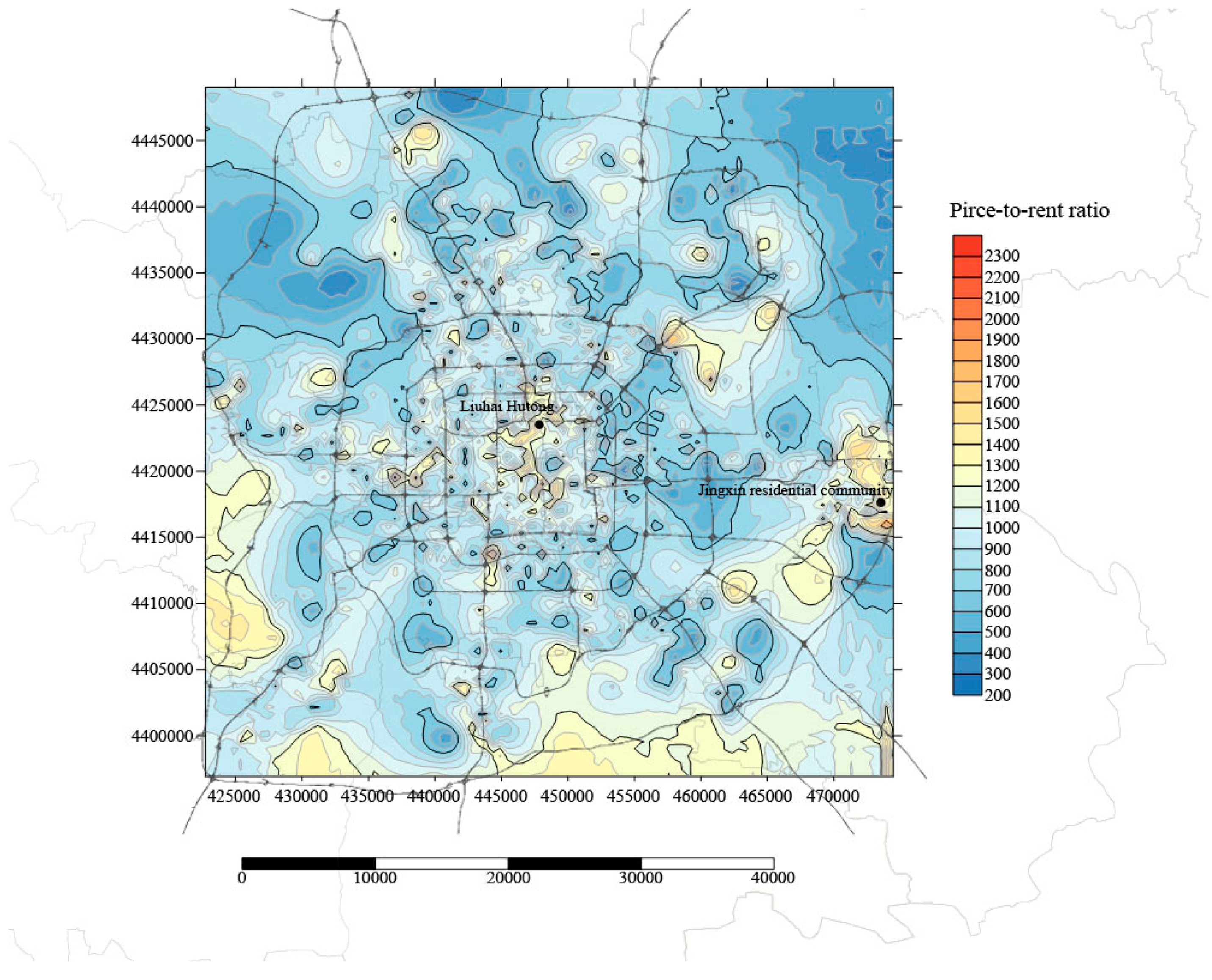
The price-to-rent ratio reflects the relative affordability of purchasing and renting a house in a given housing market. It is calculated as the ratio of the housing price per square meter of floor area to monthly housing rent per square meter, which is useful for housing tenure choice. It is usually used to measure the health of the real estate market in a region. Generally speaking, a lower value of price-to-rent ratio suggests that a place is more favorable to homeowners, and a high value of this ratio suggests a beneficial environment for renters. Thus, a higher price-rent ratio indicates a greater possibility of bubble in the price of a house. Internationally, it is generally believed that a price-to-rent ratio ranging from 200–300 indicates that the real estate market in a certain region is in good condition. If the price-to-rent ratio in a certain region is higher than 300, then it means that real estate bubble begins to appear; when this ratio is below 200, this region is favorable to homeowners. The price-to-rent ratio in Beijing averages 917, indicating a big real estate bubble in Beijing, and it is less favorable to housing purchasers. The spatial trend (Figure 3), contour map (Figure 4), and its three-dimensional (3D) display (Figure 5) of price-rent ratio are presented below. The price-to-rent ratio exhibits the following spatial pattern:

(1)

The price-to-rent ratio generally displays a disordered, homogenous, and flat spatial distribution. In Figure 3, the east–west direction (green line) and the north–south direction (blue line) are almost linearly distributed, indicating that the price-to-rent ratio within the sixth ring in Beijing presents a relatively homogeneous distribution in space. As we can see from the contour map (Figure 4) and 3D map (Figure 5), the high-value area and the low-value area are staggered with each other, further showing a chaotic mottled spatial distribution of price-to-rent ratio. This can be easily understood. Since both the housing prices and housing rent show a polycentric declining distribution, the price-to-rent ratio calculated by the ratio of housing prices to housing rent shows a relatively flat distribution.

(2)

The peak of price-to-rent ratio not only appears in the inner city, but also in the outer area. Areas with a price-to-rent ratio that is higher than 1000 are scattered not only in inner city areas (such as the alley of Xicheng District), but also in areas, such as the Southern sixth ring road (such as Daxing District), Western sixth ring road (such as Shijingshan District), and Eastern sixth ring road (such as Tongzhou District). However, the reasons leading to this situation are quite different. The reason for the high price-to-rent ratio in some residential communities in the inner city is that the housing prices of these residential communities are relatively high. For example, the housing prices in the LiuHai hutong (meaning “alley”) residential community, located in the Xicheng District in the inner city, are as high as 151,000 yuan/m², with a housing rent of 90 yuan/(m²*month), thus leading to a price-to-rent ratio of up to 1678. Meanwhile, the housing price of the Jingxin residential community, located in the Tongzhou District, is 54,790 yuan/m², with a housing rent of 30 yuan/(m²*month) and a price-to-rent ratio up to 1826. Therefore, the peak of price-to-rent ratio might not always appear in high-priced areas, and rent is also a very important factor affecting the sales ratio. For Beijing’s Daxing, Fangshan, Tongzhou, and other outer suburbs, as compared to the inner city, there is not enough industrial support and employment, resulting in lower housing rent.

5. Results

After a comparative analysis of the spatial distribution of housing prices and housing rent, the differences among the influencing factors on the two prices are further discussed in this section. The hedonic price model and quantile regression were employed, respectively, for comparing and investigating the impact of microlevel influencing factors across the complete distribution of housing prices and housing rent, and further determine how homeowners and renters value each factor in Beijing. Firstly, we started from a traditional hedonic price model based on OLS estimation through the Stata software (

Table 5. Estimation of housing prices and housing rent in the hedonic price model.

Rent Price	Housing Price	Housing Rent
Area	−0.2532 ***	−0.4774 ***
	(−37.32)	(−100.66)
Age	−0.1131 ***	−0.1057 ***
	(−30.84)	(−21.99)
Bedroom	0.0392 ***	0.0983 ***
	(12.06)	(32.05)
Mjob	−0.0556 ***	−0.0650 ***
	(−31.16)	(−24.45)
Subjob	−0.0177 ***	−0.0366 ***
	(−18.04)	(−13.93)
Bus	0.0208 ***	−0.0142 ***
	(10.52)	(−4.65)
Subway	−0.0286 ***	−0.0505 ***
	(−12.65)	(−13.57)
Park	−0.0251 ***	−0.0008
	(−10.76)	(−0.2)
Hospital	−0.0471 ***	−0.0574 ***
	(−21.46)	(−15.43)
School	−0.1124 ***	−0.1101 ***
	(−51.76)	(−34.11)
Cschool	0.3122 ***	0.1180 ***
	(35.05)	(8.72)
Dschool	0.0998 ***	0.0546 ***
	(23.68)	(8.18)
Constant	14.5372 ***	9.1242 ***
	(384.52)	(187.5)
Adjusted R2	0.6163	0.7665

Note: *** denotes significance at the 1% level.

). Then, we analyzed conditional housing prices and housing rent at the following quantiles: 0.1, 0.2, 0.3, 0.4, 0.5, 0.6, 0.7, 0.8, and 0.9, which are correspondingly denoted by Q10–Q90. The quantile regression results of housing prices and housing rent are also reported in

Table 6. Estimation of house price using the quantile model.

House Price	Q10	Q20	Q30	Q40	Q50	Q60	Q70	Q80	Q90
Area	−0.2624 ***	−0.2494 ***	−0.2494 ***	−0.2428 ***	−0.2498 ***	−0.2604 ***	−0.2667 ***	−0.2537 ***	−0.2401 ***
	(−25.01)	(−28.79)	(−33.19)	(−34.42)	(−32.47)	(−32.03)	(−30.34)	(−24.29)	(−18.67)
Age	−0.0719 ***	−0.0799 ***	−0.0955 ***	−0.1052 ***	−0.1121 ***	−0.1241 ***	−0.1319 ***	−0.1301 ***	−0.1528 ***
	(−12.81)	(−16.56)	(−23.07)	(−27.35)	(−26.94)	(−28.6)	(−28.3)	(−23.57)	(−22.37)
Bedroom	0.0090 *	0.0134 ***	0.0211 ***	0.0238 ***	0.0336 ***	0.0424 ***	0.0529 ***	0.0554 ***	0.0610 ***
	(1.77)	(3.19)	(5.82)	(7.04)	(9.11)	(10.94)	(12.73)	(11.15)	(10.03)
Mjob	−0.0509 ***	−0.0545 ***	−0.0601 ***	−0.0620 ***	−0.0651 ***	−0.0692 ***	−0.0725 ***	−0.0748 ***	−0.0710 ***
	(−12.54)	(−17.77)	(−24.82)	(−30.15)	(−32.16)	(−36.09)	(−38.79)	(−38.17)	(−32.36)
Subjob	−0.0241 ***	−0.0210 ***	−0.0193 ***	−0.0173 ***	−0.0166 ***	−0.0157 ***	−0.0149 ***	−0.0143 ***	−0.0080 ***
	(−15.24)	(−15.97)	(−17.13)	(−16.73)	(−14.92)	(−13.68)	(−12.57)	(−10.82)	(−5.55)
Bus	0.0168 ***	0.0194 ***	0.0209 ***	0.0189 ***	0.0198 ***	0.0212 ***	0.0207 ***	0.0216 ***	0.0132 ***
	(5.8)	(7.79)	(9.55)	(9.17)	(8.81)	(8.97)	(8.06)	(6.98)	(3.58)
Subway	−0.0329 ***	−0.0307 ***	−0.0320 ***	−0.0320 ***	−0.0313 ***	−0.0298 ***	−0.0286 ***	−0.0274 ***	−0.0224 ***
	(−9.02)	(−10.15)	(−12.22)	(−13.29)	(−12.23)	(−11.34)	(−10.41)	(−8.52)	(−5.62)
Park	−0.0170 ***	−0.0166 ***	−0.0200 ***	−0.0184 ***	−0.0180 ***	−0.0252 ***	−0.0300 ***	−0.0332 ***	−0.0284 ***
	(−4.45)	(−5.22)	(−7.42)	(−7.42)	(−6.8)	(−9.22)	(−10.34)	(−9.93)	(−7.64)
Hospital	−0.0410 ***	−0.0373 ***	−0.0384 ***	−0.0408 ***	−0.0442 ***	−0.0441 ***	−0.0464 ***	−0.0511 ***	−0.049 ***
	(−12.04)	(−13)	(−15.31)	(−17.56)	(−17.78)	(−17.35)	(−17.61)	(−16.82)	(−13.81)
School	−0.0900 ***	−0.096 ***	−0.0978 ***	−0.1031 ***	−0.1071 ***	−0.1100 ***	−0.1126 ***	−0.1173 ***	−0.1500 ***
	(−20.88)	(−28.85)	(−35.95)	(−42.95)	(−43.47)	(−45.35)	(−46.01)	(−43.78)	(−50.22)
Cschool	0.2947 ***	0.2912 ***	0.2989 ***	0.2967 ***	0.2928 ***	0.3083 ***	0.3362 ***	0.3452 ***	0.3747 ***
	(22.59)	(26.03)	(30.3)	(32)	(29)	(29.14)	(29.62)	(25.55)	(22.77)
Dschool	0.0693 ***	0.0953 ***	0.1032 ***	0.1091 ***	0.1138 ***	0.1160 ***	0.1122 ***	0.1030 ***	0.0780 ***
	(11.69)	(18.25)	(22.28)	(24.94)	(23.81)	(23.14)	(20.85)	(16.04)	(9.91)
Constant	14.0783 ***	14.0988 ***	14.2611 ***	14.3609 ***	14.5043 ***	14.6952 ***	14.8610 ***	14.9546 ***	15.1857 ***
	(226.49)	(276.57)	(328.86)	(358.92)	(338.31)	(330.84)	(314.57)	(271.8)	(229.47)
Pseudo R2	0.3958	0.4004	0.4036	0.4068	0.4087	0.4085	0.4073	0.396	0.3686

Note: *, *** denote significance at the 10% and 1% levels, respectively.

and

Table 7. The rental estimated using the quantile model.

Rent Price	Q10	Q20	Q30	Q40	Q50	Q60	Q70	Q80	Q90
Area	−0.4935 ***	−0.5014 ***	−0.5073 ***	−0.5063 ***	−0.5000 ***	−0.4919 ***	−0.4885 ***	−0.4822 ***	−0.4670 ***
	(−79.15)	(−101.14)	(−106.66)	(−126.00)	(−105.12)	(−79.40)	(−74.99)	(−72.57)	(−38.04)
Age	−0.0869 ***	−0.0856 ***	−0.0968 ***	−0.1012 ***	−0.1036 ***	−0.1069 ***	−0.1059 ***	−0.1130 ***	−0.1234 ***
	(−13.43)	(−15.92)	(−19.18)	(−24.3)	(−21.49)	(−17.34)	(−16.96)	(−18.64)	(−12.44)
Bedroom	0.0639 ***	0.0709 ***	0.0760 ***	0.0826 ***	0.0912 ***	0.1025 ***	0.1117 ***	0.1256 ***	0.1464 ***
	(14.1)	(19.93)	(23.06)	(30.89)	(29.64)	(26.13)	(27.95)	(31.9)	(21.09)
Mjob	−0.0424 ***	−0.0524 ***	−0.0537 ***	−0.0581 ***	−0.0673 ***	−0.0770 ***	−0.0882 ***	−0.0941 ***	−0.1096 ***
	(−8.78)	(−14.66)	(−16.81)	(−23.44)	(−25.3)	(−24.7)	(−31.12)	(−40.68)	(−33.08)
Subjob	−0.0227 ***	−0.0262 ***	−0.0284 ***	−0.0322 ***	−0.0320 ***	−0.0350 ***	−0.0360 ***	−0.0370 ***	−0.0476 ***
	(−6.19)	(−8.81)	(−10.29)	(−14.11)	(−12.13)	(−10.44)	(−10.76)	(−12.06)	(−8.93)
Bus	−0.0057	−0.0131 ***	−0.0153 ***	−0.0144 ***	−0.0150 ***	−0.0187 ***	−0.0205 ***	−0.0222 ***	−0.0219 ***
	(−1.21)	(−3.63)	(−4.62)	(−5.34)	(−4.89)	(−4.88)	(−5.42)	(−6.49)	(−3.78)
Subway	−0.0545 ***	−0.0496 ***	−0.0508 ***	−0.0533 ***	−0.0498 ***	−0.0489 ***	−0.0508 ***	−0.0458 ***	−0.0491 ***
	(−8.98)	(−10.59)	(−12.02)	(−15.87)	(−13.32)	(−10.69)	(−11.33)	(−10.71)	(−6.77)
Park	0.0202 ***	0.0138 ***	0.0117 ***	0.0105 ***	0.0064*	0.001	−0.004	−0.0128 ***	−0.0255 ***
	(3.78)	(3.22)	(2.91)	(3.19)	(1.68)	(0.2)	(–0.83)	(–2.75)	(–3.13)
Hospital	−0.0570 ***	−0.0529 ***	−0.0549 ***	−0.0534 ***	−0.0501 ***	−0.0435 ***	−0.0404 ***	−0.0435 ***	−0.0406 ***
	(−9.31)	(−11.35)	(−13.1)	(−16.05)	(−13.4)	(−9.35)	(−8.71)	(−9.58)	(−5.14)
School	−0.1041 ***	−0.1038 ***	−0.1064 ***	−0.1078 ***	−0.1085 ***	−0.1088 ***	−0.1088 ***	−0.1148 ***	−0.1144 ***
	(−18.12)	(−24.72)	(−28.44)	(−36.66)	(−33.52)	(−27.9)	(−29.27)	(−34.65)	(−23.02)
Cschool	0.1212 ***	0.0941 ***	0.0992 ***	0.1144 ***	0.1249 ***	0.1561 ***	0.1695 ***	0.1648 ***	0.1251 ***
	(6.97)	(6.37)	(7.08)	(9.81)	(9.22)	(9.03)	(9.7)	(9.88)	(4.47)
Dschool	0.0487 ***	0.0566 ***	0.0650 ***	0.0680 ***	0.0673 ***	0.0680 ***	0.0608 ***	0.0511 ***	0.0414 ***
	(5.53)	(7.88)	(9.42)	(11.82)	(10.05)	(7.96)	(7.07)	(6.3)	(3.07)
Constant	8.4511 ***	8.6683 ***	8.8698 ***	9.0015 ***	9.0706 ***	9.1863 ***	9.3433 ***	9.5477 ***	9.8820 ***
	(119.99)	(154.84)	(171.91)	(212.78)	(185.75)	(147.72)	(148.59)	(160.09)	(97.98)
Pseudo R2	0.4951	0.5276	0.5445	0.5532	0.5557	0.5554	0.5508	0.5446	0.5407

Note: *** denotes significance at the 1% level.

.

5.1. Hedonic Price Model of Housing Prices and Housing Rent

In the hedonic price model of housing prices (Table 5), all of the estimated coefficients are statistically significant at the 1% level. R² suggests that the hedonic price model accounts for 61.63% of the variability of the log of housing prices, which is reasonably high for micro data. Coefficients of structural characteristics, locational characteristics, neighborhood characteristics, and school dummies all have the expected signs. The larger the living area is, the lower the housing price per square meters. A higher building age indicates an older house; thus, the coefficient for age is expected to be negative in the hedonic price model of housing prices. An additional bedroom increases the house value by approximately 3.92%. Holding everything constant, housing prices decrease by approximately 0.056%, 0.018%, and 0.029%, respectively, as the distance from the house to the nearest major employment center, subordinate employment center, and subway station increases by 1%. However, distance to the nearest bus stop has a positive influence on housing prices, possibly because of noise disturbance. Similarly, housing prices decrease by 0.025%, 0.047%, and 0.112%, respectively, as the distance from the house to the nearest park, hospital, and school decreases, which offers benefits and conveniences to families and their children. There is a 31.22% increase in the housing prices of residential communities located in the school attendance zones of city-level key elementary schools (meaning high-quality education), higher than the 9.98% increase in housing prices if a house is located in the school attendance zones of district-level key elementary schools (meaning medium-quality education).

In the hedonic price model of housing rent (Table 5), all of the estimated coefficients except Park are significant at the 1% level. R² suggests that the hedonic price model accounts for 76.65% of the variability of housing rent in log form. The larger the living area is, the lower the housing rent per square meters. The building age is negative, indicating that the older the house is, the lower the housing rent. The number of bedrooms has a positive effect on housing rent. Other estimated coefficients of variables, like proximity to employment center and public facilities except bus and park, follow a pattern similar to those in the hedonic price model of housing prices. When compared to homeowners, proximity to a bus stop is still important to renters. Park, representing enjoyable green views, is not significant in the hedonic model of housing rent, suggesting that renters are not so concerned about whether the rented house is close to a park. Interestingly, high school quality and medium school quality can also be capitalized into housing rent to some extent, even though renters’ children cannot be admitted to school if they do not buy a house in school attendance zones.

There are some similarities and differences in the impact of microlevel influencing factors on housing prices and housing rent, from which we can infer the preferences of homeowners and renters. They both prefer properties with a good structure, such as a larger living area, newer house, more bedrooms, a good location, good neighborhood facilities, as well as a good school attendance zone. Interestingly, even though renters’ children in Beijing cannot get enrolled in public school, school quality is still capitalized into the rental price. But, the price premium of school quality for homeowners exceeds the premium for renters, indicating that homeowners are willing to pay for more price premiums of school quality than renters because homeowners have lower expectation for mobility and renters have higher expectation for mobility, which will affect their tenure choice. Moreover, what is different is that proximity to a park has a positive effect on housing prices, but it has no positive effect on housing rent on average. A park is a type of green space with ecological, recreational, and cultural functionality, which can maintain moderate humidity and reduce noise. Thus, proximity to a park increases housing prices. However, renters who are always under greater pressure to survive in Beijing hope that renting a house can meet their basic needs, thus paying little attention to and showing less strong demand for closeness to a park as compared to homeowners. However, OLS estimation fails to identify the differential effect of the independent variables across the conditional distribution of housing prices and housing rent. Moreover, OLS assumes homoscedasticity, which means that the conditional variance of the disturbance terms is constant. We conducted a Breusch–Pagan test and a White test on Equation (1) and the test result showed that we should reject the null hypothesis of homoscedasticity. Last, OLS estimation is sensitive to extreme values and outliers. Therefore, we needed to use the quantile regression model to further our estimation.

5.2. Quantile Regression Model of Housing Prices and Housing Rent

Quantile regression analyzes the characteristics across the complete distribution of housing prices and housing rent. Quantile regression has allowance for heteroskedasticity in the disturbances [61] and it is robust to outliers. Therefore, we used quantile regressions and display estimates of coefficients at different deciles in Table 6 and Table 7. The results in Figure 6 and Figure 7 show coincidence with those in Table 6 and Table 7, respectively. As can be seen from the tables and figures, most of the variables have different coefficients from the estimation of OLS and change greatly across quantiles. In order to describe the regression coefficients of the variables under different quantiles more accurately, the variation of regression coefficients and the confidence interval are presented. The influence of each variable on housing prices and housing rent is analyzed in detail below.

(1) Quantile Regression of Housing Prices

We first examined the regression coefficients of locational characteristics. The results (Table 6) showed that higher-priced homeowners value the building age and number of bedrooms more than lower-priced homeowners. The living area shows a significant negative impact on housing prices across all the quantiles, with no obvious trend in the coefficients. Obviously, there is a decreasing trend in the coefficients of building age and an increasing trend in the coefficients of the number of bedrooms. For every increase of one year in building age, the home value will decrease by approximately 7.19% at the 0.1 quantile and 15.28% at the 0.9 quantile. An additional number of bedrooms add home value by approximately 0.9% at the 0.1 quantile and 6.1% at the 0.9 quantile. The result showed that higher-priced homeowner consumers are more inclined to live in a newly built house or a house with more bedrooms.

As to locational characteristics, the regression coefficients of a major employment center, subordinate employment center, and subway station are all significantly negative at all quantiles, while the regression coefficients of a bus station are significantly positive at all quantiles. Location near a major employment center contributes more value to the price of housing at higher quantiles, while house prices at lower quantiles are more sensitive to subordinate employment centers and subway stations. This is reasonable because higher-priced homeowners prefer a good location and are more likely to own private cars, lowering the demand for the convenience of public traffic. The regression coefficients of bus are statistically significant and positive, indicating that the proximity to a bus stop may have negative effects on housing prices because of noise.

When it comes to neighborhood characteristics, we can see that higher-priced homeowners are more concerned with neighborhood characteristics. The regression coefficients of distance from house to the nearest park, hospital, and key elementary school are statistically significant and negative at all quantiles, all with an obvious downward trend. Obviously, the capitalization of park, hospital, and key elementary school accessibility is larger in higher-priced homeowners.

The impact of school dummy variables on housing prices is different, with a upward trend in the coefficients of a city-level key elementary school (meaning high-quality education) and an inverted U shape in the coefficients of a district-level key elementary school (meaning medium -quality education). For instance, high-quality education raises the value of houses by about 29.47% at the 0.1 quantile and approximately 37.47% at the 0.9 quantile, while medium-quality education adds to the value of houses by 6.93% at the 0.1 quantile, 11.38% at the 0.5 quantile, and 7.8% at the 0.9 quantile. Therefore, higher-priced homeowners that have a strong demand for good school quality have a greater willingness to pay a purchase price premium of high-quality education than of medium-quality education.

(2) Quantile Regression of Housing Rent

Housing attributes that a renter prefers may be different from those of a homeowner. Renters or homeowners with different housing purchasing ability may have different preferences. Therefore, we needed to further explore this difference. The estimation result of quantile regression of housing rent is presented in Table 7. The results indicate that higher-priced renters prefer living in newly built houses with a larger living area, more bedrooms, in a higher school quality attendance zone, which is closer to an employment center, park, and school than lower-priced renters.

The regression coefficients of the living area and building age are negatively significant at all quantiles, and the number of bedrooms shows a significantly positive effect across all quantiles. There is an obvious upward trend in the coefficients of both the living area and the number of bedrooms, while there is an obvious downward trend in the coefficient of the number of bedrooms. From the absolute value of the coefficients, it can be deduced that lower-priced renters are more concerned with the living area, while higher-priced renters care more about the building age and number of bedrooms.

Renters usually hope to travel a short distance to work. Therefore, they are eager to live close to an employment center. The longer the distance from the house to the employment center is, the lower the rental price. Higher-priced renters have a stronger demand for proximity to a major employment center than lower-priced renters. For instance, for every 1% increase in the distance to the major employment center, the average monthly housing rent will drop by about 0.042% at the 0.1 quantile and approximately 0.11% at the 0.9 quantile, respectively. Different from homeowners, renters prefer to live close to bus stops that provide good public transit convenience. The closer to the bus stop a house is, the higher the housing rent. Proximity to a subway station also shows an advantageous effect on housing rent at all quantiles with no obvious trend indicating whether lower-priced renters or higher-priced renters all show a great demand for good accessibility to subway stations.

Quantile effects are obvious for the neighborhood characteristics. The coefficients of a park and school both show a steady decreasing trend, while the coefficient of a hospital shows an increasing trend as the quantile of the housing price increases, indicating that distance to the nearest hospital has more of an effect on lower-priced renters. The beneficial effect of park and school is much more obvious at higher quantiles of housing rent, indicating that higher-priced renters are more concerned with the living environment and proximity to school than lower-priced renters. What is more interesting is that the regression coefficients of a city-level key elementary school and district-level key elementary school are also statistically significant and positive at all quantiles. The results show that school quality may also be capitalized into rent price to some extent, even though tenants’ children are not eligible to be admitted to school. The fact that some of homeowners who have already obtained school qualifications for their children may rent out their own private house and choose to rent another house near the school in recent years has led to an increase in rent price in school attendance zones, because renting a house near school can save parents a lot of time of getting their children to school. Medium school quality has more of an impact on medium-priced renters, while higher-priced renters value higher-quality education than other renters.

5.3. Comparative Analysis

By comparing the above estimation results of housing prices and housing rent, we can find some interesting similarities and differences (

Table 8. Comparative analysis of factors influencing housing and rent prices.

Variables	Housing Price				Housing Rent
	OLS	Lower	Medium	Higher	OLS	Lower	Medium	Higher
Area	–	no obvious difference			–			●
Age	–	●			–			●
Bedroom	+			●	+			●
Mjob	–			●	–			●
Subjob	–	●			–			●
Bus	+			●	–			●
Subway	–	●			–	no obvious difference
Park	–			●	Insignificant			●
Hospital	–			●	–	●
School	–			●	–			●
Cschool	+			●	+			●
Dschool	+		●		+		●

Note: “+” denotes positive significant influence; “–” denotes negative significant influence; “•” denotes the variable has a stronger effect on corresponding quantiles of housing price or housing rent. If there is no “•”, the impact of variables on housing prices or housing rent at different quantiles shows no obvious difference.

). On average, both homeowners and renters prefer properties with a good structure, such as a larger living area, newer house, more bedrooms, a good location, good neighborhood facilities, as well as a good school attendance zone. What is different is that the park and school quality coefficients for homeowners are higher in magnitude than the coefficients for renters, while the coefficients of the living area, number of bedrooms, and proximity to employment centers, public transportation (bus, subway), and hospital are higher in magnitude than the coefficients for homeowners. Moreover, proximity to a bus stop has the opposite impact on housing prices and housing rent. Proximity to a park has no impact on housing rent. When compared to homeowners, renters prefer to live close to bus stops that provide good public transit convenience and show almost no demand for proximity to a park, while homeowners, who probably have private cars, prefer to live away from bus stops, probably because of noise disturbance and a tendency to live near a park.

If we compare the estimation results across quantiles, we can find that both higher-priced homeowners and higher-priced renters are more willing to live in property with a larger number of bedrooms, proximity to a major employment center, park, or school, as well as being located in a school attendance zone with higher school quality. Lower-priced homeowners are more sensitive to the building age of house and the proximity to the subordinate employment center and subway station, while lower-priced renters value closeness to a hospital. Both medium-priced homeowners and medium-priced renters are concerned more about medium school quality than others.

6. Conclusions and Discussion

The long-term unbalanced development between the housing sales market and housing rental market has constrained the healthy development of the real estate market since the reform of the residential allotment system. For a long time, the housing sales market has gained considerable interest and concern, while the housing rental market has often been ignored in China. With the acceleration of urbanization, more and more migrants are pouring into Beijing to seek employment opportunities, thus generating a growing demand for renting houses. However, homeowners in the housing sales market and renters in the housing rental market likely differ in terms of preferences. Exploring and comparing how the microlevel influencing factors impact housing prices and housing rent is of crucial importance for sustainable urban planning and management, so that we can investigate how homeowners and renters value each factor.

This study makes contributions to this research field by comparing and examining the spatial distributions of housing prices and housing rent, as well as the price-to-rent ratio, and comparing the impact of microlevel influencing factors across the complete distribution of housing prices and housing rent using a comprehensive public large sample data. Using 16,475 house purchase transaction and 7129 rent transaction data, as well as the average housing price and rent price data of 5196 residential communities in Beijing, China, this study first explores the spatial patterns of housing prices and housing rent employing the methods of Kriging spatial interpolation and spatial trend analysis, and it then compares the impact of determinants on housing prices and housing rent using the hedonic price model and quantile regression. Three main findings stand out in our paper. Firstly, the spatial patterns of housing prices and housing rent both exhibit a decentralized distribution with multiple centers and show obvious north–south differences between south and north Chang’an Avenue. However, the gradient of housing rent is much slower than that of housing prices. Urban rail transit and urban expressway have obviously contributed a great deal to the increase in housing prices and housing rent. The residential communities with high housing prices do not necessarily have high housing rent. The price-to-rent ratio in Beijing displays a disordered, homogenous, and flat spatial distribution. Secondly, microlevel influencing factors have a different impact on housing prices and housing rent. That is to say, homeowners and renters differ in terms of some preferences. Homeowners prefer a higher-quality living environment (e.g., good accessibility to park, away from noise disturbance), as they have higher living standards than renters, while renters are not interested in closeness to a park, but more concerned with proximity to employment centers and good public transit convenience than homeowners. Moreover, school quality can be capitalized both into housing prices and housing rent, but the price premium of school quality for homeowners exceeds the premium for renters. Thirdly, the impact of characteristics varies differently across the conditional distribution of housing prices and housing rent, suggesting that it is very useful to perform the estimation of conditional quantile functions apart from OLS (the conditional mean). For example, when compared to lower-priced homeowners and lower-priced renters, both higher-priced homeowners and higher-priced renters are more willing to live in properties with a larger number of bedrooms, proximity to a major employment center, park, or school, as well as located in a school attendance zone with higher school quality.

The reasons can be summarized, as follows. There is a strong speculation in the housing sales market in Beijing, while there is almost no speculation in the rental market. Thus, price-to-rent is very high, with a big bubble in the housing sales market. According to the 2016 National Real Estate Investment Rate of Return Survey Report, in the second half of 2016, the return on one-year leases of ordinary residential buildings in Beijing was only 1.6% and the return on long-term lease rate of ordinary residential buildings in Beijing was 5.4%. However, the return on resale after a five-year lease of ordinary residential buildings in Beijing was as high as 11.4%. Lower rental income expectations and higher transaction costs have reduced economic incentives of property owners for renting, which have increased house vacancies and thus limited the flow of houses from the sales market to the rental market. Moreover, homeowners and renters have different housing affordability, which has determined differences in terms of their housing preferences. Homeowners in Beijing are mainly medium or higher income groups of society who prefer a higher quality of life and education resources, while renters are mainly low-income groups, such as graduate college students and migrant workers, who have to care more about the living and commuting cost. For example, in Beijing, school attendance zoning is a dominant factor fueling the housing market. Parents have a greater willingness to pay a purchase price premium of high-quality education, creating educational and economic segregation. Even though renters’ children in Beijing cannot get enrolled in public school, school quality is still capitalized into the rent price, because homeowners may choose to rent a house near the school to save time for getting children to school.

The findings of this study are beneficial for sustainable urban planning and management. On the one hand, the government should make housing decisions according to the different housing preferences of homeowners and renters. For instance, renters prefer the convenience of transportation to proximity to parks. Therefore, the government should make site selection decisions for public rental housing on the basis of good accessibility of transit rather than closeness to a park. On the other hand, to cool the fueling price of school district houses and eliminate speculation in the housing sales market, we suggest adjusting and optimizing the “nearby enrollment” policy to promote the equalization of educational opportunities. Policies such as multiple school attendance zones with the enrollment lottery system should be implemented to strengthen the uncertainty of school attendance zones and reduce the psychological expectation of being enrolled in a high-quality school just through buying a house in the “school attendance zone”. At the same time, we should improve the rights and interests of renters. With a pilot scheme of “people who rent houses should have equal rights to people who buy houses” in Guangzhou, China, the housing rental market is expected to grow, but that means there will be a reallocation of public resources between property owners and renters, especially in the reallocation of education. This is a challenge facing the Chinese government.