Ancient Use of Natural Geothermal Resources: Analysis of Natural Cooling of 16th Century Villas in Costozza (Italy) as a Reference for Modern Buildings

Abstract

The geothermal cooling system of six 16th century villas in Costozza (Vicenza, Italy) is analysed and modelled using computational fluid dynamics and referring to in-field monitoring data. The system passively cools the villas in summertime by means of underground ducts connected to the caves present in the nearby hills. It still perfectly works in Villa Aeolia, which is analysed here in more detail. The outcomes permit us to better understand the functioning conditions and to improve the conservation of the villas as a whole. Furthermore, the ancient cooling system can be used as a reference for how geothermal renewable resources can be used to improve indoor comfort and limit energy consumption in modern buildings in a temperate climate. A macroscopic analysis of the global airflow system as well as a detailed analysis of Villa Aeolia are developed. All results are validated with analytical methods, numerical methods, and with past experimental records. The system can provide fresh airflow rates that cool the walls of the room and maintain the temperature below 20 ${}^{°}$C even on hot summer days. An advantage is that the system works in a self-adaptive way, the airflow increases when the outdoor temperature increases. This self-adjustment allows us to compare the cooling system to a modern environmental control system.

1. Introduction

The growing need to reduce energy consumption in buildings has promoted interest in passive geothermal cooling and natural ventilation techniques to improve indoor comfort. Earth air heat exchangers (EAHEs) can capture heat from and/or dissipate heat to the ground, preheating the air in winter and cooling it in summer. The technique uses the high heat capacity of earth and the consequently the fact that its temperature remains fairly constant throughout the year starting from a depth of 1.5 to 2 m, falling around the mean air temperature of the site [1]. In the past two decades, a great deal of research has been done to develop analytical and numerical models for the analysis of EAHE systems and their performance, and their design is still current today [2,3].

Soltani [4] presents a comprehensive investigation of geothermal heating and cooling systems, with an overview of ground source heat pumps and ground heat exchangers. Several factors that can enhance the installation soundness and thermal performance of geothermal heating or cooling systems are discussed. Kaushal [5] gives a comprehensive review of experimental and analytical studies on geothermal heat exchangers. Bordoloi collects the latest advancements, presenting different combinations of EAHEs and their thermal performances [6]. The reviews of Ozgener [7], Sigh [8], Ascione [9], and Yusof [10] present studies conducted on EAHEs (earth to air heat exchanger systems) in Turkey, India, Italy, and Malaysia, respectively, giving some indication about performances, costs, and perspectives.

In addition, many applications have been developed showing the interest in employing these systems. As an example, Alajmi et al. [11] show that the soil has the potential to reduce cooling energy demand in a typical house in Kuwait by 30% over the peak summer season. Moreover, Dorra et al. [12] propose a design for desert Egyptian dwellings that accommodate the hot dry climate by incorporating passive elements and by using stabilised earth blocks as a local building material. In [13], the use of low-enthalpy geothermal energy that consists of converting mine galleries in Spain into underground heat exchangers is described and analysed. On the other hand, geothermal systems coupled to other natural environmental forces to cool or heat the air supplied to buildings have been known since the times of the ancients. Egyptians used the thermal difference between the day and night to ventilate the construction works of their underground tombs [14,15]. Iranians used wind towers and underground ducts for passive cooling and ventilation sometimes integrated with the “qanat” (an underground channel to collect water) already in the fourth millennium B.C. [16,17].

More recently in Sicily (Italy) during the middle age, the underground irrigation channels called qanats, brought here by Arabs, were associated with the underground structures called Scirocco Chambers, vaulted and well-ventilated underground rooms [18,19] where a cool microclimate was available for nobles during hot summer days. Moreover, another example of a natural cooling system applied to buildings in Italy came from the Renaissance. It consists of an open loop EHAE excavated in the rock that ventilates and cools some ancient villas in Costozza near Vicenza in North-East Italy. All these are examples of how natural local resources can be utilised in a smart and bioclimatic way. The system in Costozza is analysed here. Its behaviour and performances are investigated using two tools usually used for the study of natural ventilation in buildings: computational fluid dynamics and field measurements.

Considering historical buildings, we can find various applications of these tools showing their potentiality in the analysis of airflow patterns. One example is the work of Balocco [20,21]. She developed an analysis of Palazzo Pitti in Florence, modelling the interior environment contributing to tapestry preservation [22]. The same author [23] investigated the distribution and the air velocity and temperature distributions inside Palazzo Marchese in Palermo (Italy).

Ref. [24] studied by CFD the influence on frescoes conservation of HVAC adoption for the environmental control system inside the Camera Picta in the San Giorgio Castle in Mantua.

Pagliaro [25,26] used computational fluid dynamics to support archaeologists in their effort to better understand how ancient warehouses were built, managed, and used.

Authors in [27,28] studied the “hórreos”, bioclimatic structures for drying and preserving cereals used in Galicia (Spain). In these studies, the CFD techniques were used to determine the influence of the environment (humidity and solar radiation) on the functioning of the granary and also to evaluate the architecture of the floor. The analyses were coupled with a large experimental campaign done in a real Galician granary, remembering the importance of the calibration of the model.

Oetelaar in [29] explores the thermal environment of a replica Roman bath resulting from purely subcutaneous convective heating by modelling the bath using computational fluid dynamics, providing further knowledge about an alternative heating, ventilation, and cooling (HVAC) system and improving the understanding of ancient Roman baths.

Additionally, the studies of D’Agostino [30] are focused on the ventilation strategies in the microclimate of the Crypt of Lecce Cathedral (South Italy) built in 1114 by the Normans on a pre-existing underground structure. The crypt was modelled using computational fluid dynamics tools to determine how to improve the indoor conditions controlling the ventilation and to preserve the monument.

In fact, once the ventilation systems in a historic building are known, it is advisable to restore or improve these technologies as expressed in the following papers. Soltani [31] used CFD to develop, starting from a traditional wind tower, a new apparatus with a moistened pad able to optimise the cooling wind use, realising the desired comfort conditions. Laurini [32] analyses the historical Kalteyer House located in San Antonio (Texas) by using CFD. This is also an excellent example of a passive stack effect design for a residential building. Still, ref. [33] uses Thomson analyses with CFD for the natural ventilation of Royal Wanganui Opera House built in 1899 in New Zealand [34], showing that the systems with which these buildings were originally designed have the potential to meet modern-day standards of cooling and fresh air. Similarly, Käferhaus studied the reactivation of the natural ventilation in the historical building SchÃnbrunn Castle built in 1881 in Vienna (Austria) [35]. Some other research deals with the CFD simulation of heritage buildings considering different HVAC strategies and showing the potential of the CFD tools to predict air flow paths and the thermo-hygrometric fields in the indoor environment, such as the work of [36] about the indoor environment of the museum Palazzo Madama in Torino (Italy).

Moreover, Tronchin [37] studied the Malatestiana Library located in Cesena (Italy), XV century, using building energy performance simulation to find the state of conservation of the wooden desks and parchments without any HVAC system. Sciurpi [38] created a model suitable for the dynamic energy simulations of the Corridoio Vasariano (Firenze), calibrating it with environmental monitoring inside the building. In general, CFD simulations allow the study of large confined spaces, where it is difficult to predict the indoor air flows and thermo-hygrometric fields by means of simplified models and complete measurements campaigns are complex and time-consuming [39]. Knowing the real functioning of a building can contribute to preventing its damage due to inadequate thermal and hygrometric conditions. In this context, this paper analyses the geothermal cooling systems of six 16th century villas in Costozza (Italy). The passive cooling is based on the airflow generated inside the caves near the villas called “covoli”, and it still works in Villa Aeolia, which is analysed here in more detail. The understanding of the real functioning of these systems and the set-up of a numerical model is important to improve the conservation of the villas and their overall apparatus. An important task of this work is to create an easily implementable computational model of the underground cooling system, in order to compute the mass airflow available to cool the villas in the summer season. This tool can also be generalised and applied to passive cooling systems in new buildings in areas with similar characteristics in a temperate climate. As a result, the Renaissance cooling system can be used as a reference and can contribute to diffusing these kinds of system in modern buildings, increasing indoor comfort, indoor air quality, and limiting the summer energy consumption. The first part of this work presents the previous research on the villas of Costozza, and explains the physical principle on which the cooling system is based. Subsequently, we describe the set-up of the numerical models. A macroscopic analysis of the global airflow system as well as a detailed analysis of Villa Aeolia are developed. All results are validated with analytical methods, numerical methods, and with past experimental records.

2. Materials and Methods

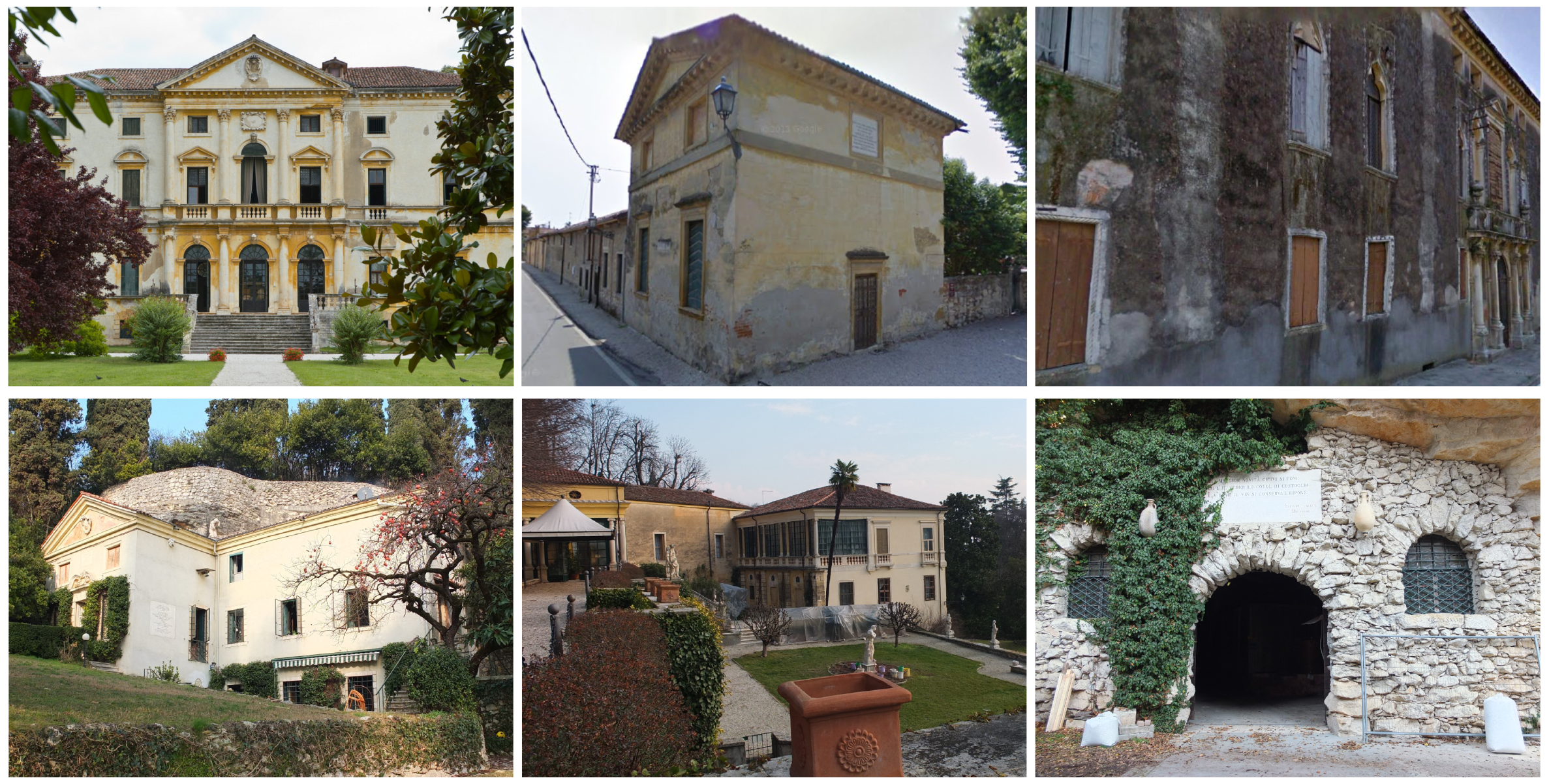
There are six villas (Figure 1) in Costozza built in the 15–17th centuries that are naturally cooled in the summertime, with the air coming from the nearby caverns and distributed by underground ducts. The villas and their underground cooling system were also known in the 16th century by Palladio [40] and Scamozzi [41]. Over the centuries, many writers became interested in the architecture of the villas and in the covoli, trying to trace back the origin of their construction and their use as evidenced by [42,43,44,45].

The villas can be divided into two groups (Figure 2 and Figure 3):

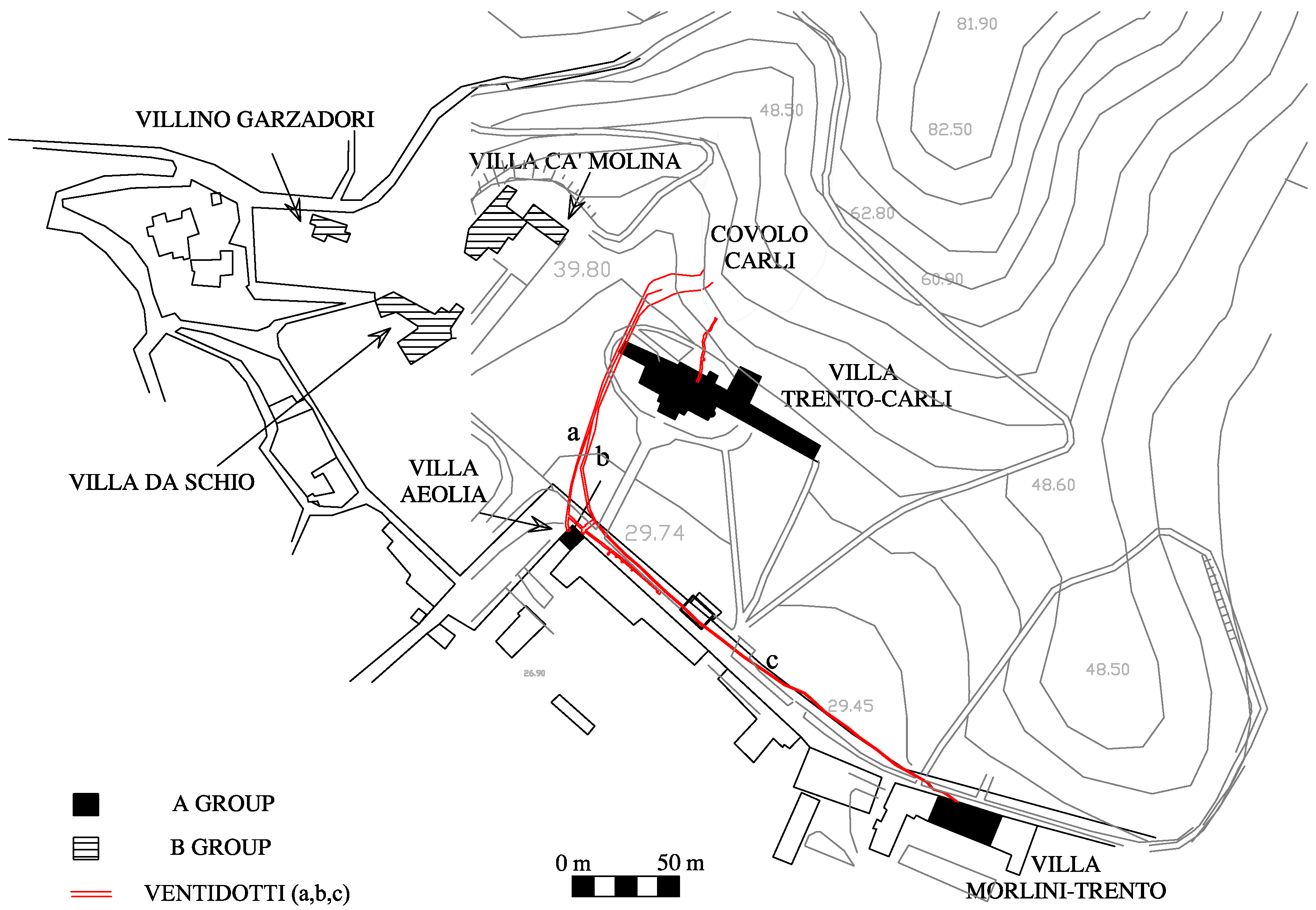
• The A group. These villas are connected to the caves with a system of underground artificial ducts with stone walls and brick vault called “ventidotti”: Villa Aeolia, Villa Morlini Trento, and Villa Trento Carli. For these buildings, fresh air comes from a cavern called Covolo Carli (or Covolo dei Venti), located at the back of the Villa Trento Carli.
• The B group. Villas leaning directly against the caves, called “covoli”: Villa Garzadori, Villa da Schio, and Villa Cà Molina. The villas are set against the mountain at different altitudes and they are directly connected by natural cracks to the Covolo del Marinali, which is located under the Da Schio park. The rooms of the villas cooled in the summer by the airflow coming from the cave are the cellars and the living room of the Villa da Schio, the cellars of the Villa Cà Molina, and the hall of Villa Garzadori.

Contrary to the notoriety of the villas, their cooling systems have not been studied in detail. Some speleological reliefs of the area were realised by the Club Speleologico Proteo of Vicenza. The first experimental campaign was performed in the summer 1981 [46,47] and the last in summer 1990 [48]. In these two experimental measurement campaigns, the thermo-hygrometric values were acquired in the artificial ducts and in some cellars of the villas of the A group, in particular Villa Aeolia and Villa Trento Carli. More recently, other works investigated the ventilation of the villas [49,50], and landscape architects and urban planners [51] highlighted that the cooling system of Costozza is a precious example for our cities, teaching us how the landscape is infrastructure for the city.

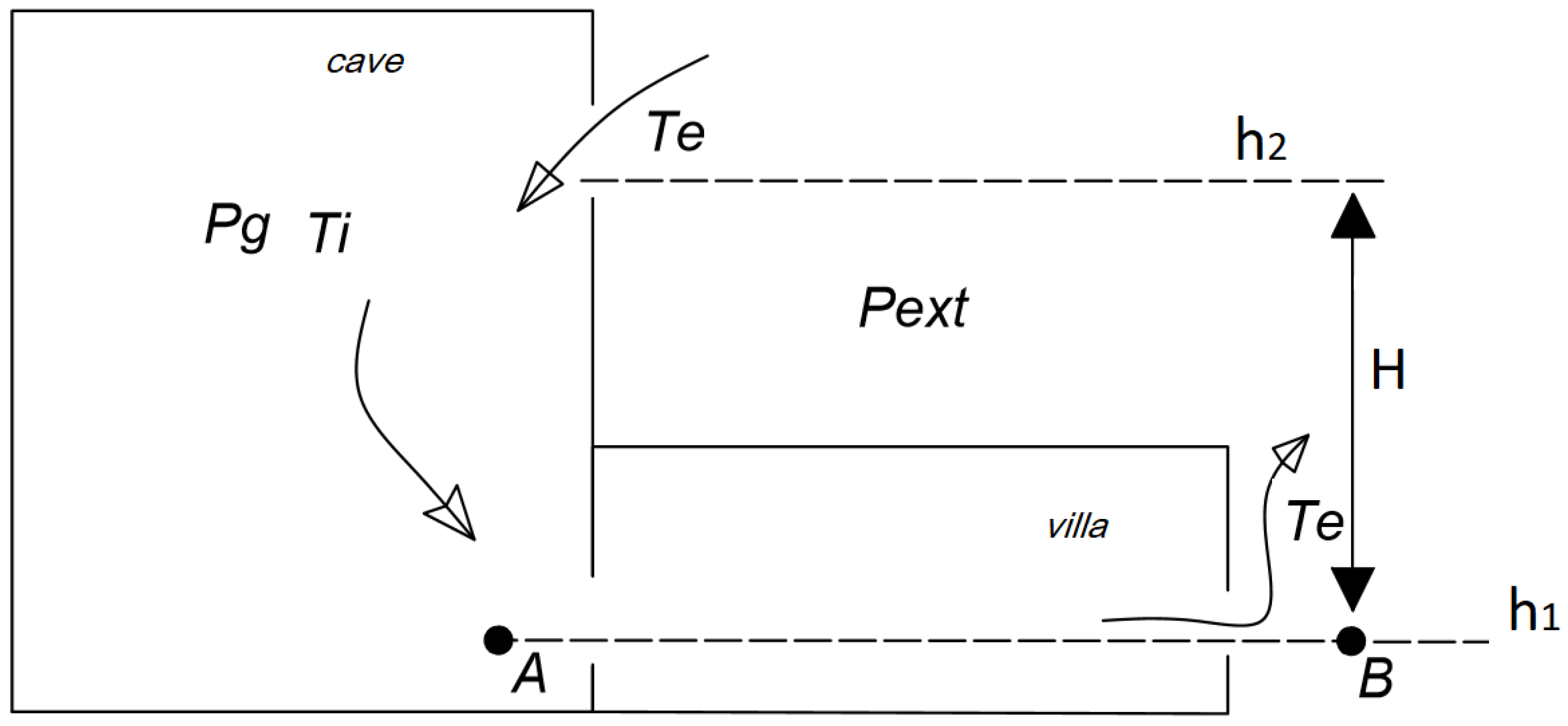
Thanks to the artificial underground ducts (i.e., ventidotti) and natural caverns (i.e., covoli), the cooled air comes from the cracks at the top of the caverns and descends to lower altitudes until it reaches the cellars of the villas. Then, the air is conveyed into different rooms to cool them. The rocks remain at a constant temperature throughout the year because of their high thermal capacity (around 11 ${}^{°}$C). By the convective thermal exchange, the air in contact with the rocks assumes the same temperature as them, and hence inside the covoli the air has a lower temperature in the hot season and higher temperature in the cold season than the outdoor air. The driving force of passive cooling is the air pressure difference inside the caverns and in the villa at the same altitude—the stack pressure. The airflow is activated by the difference of pressure between the cracks in the rock located at the top of the hills and the villa’s openings situated at their bottom with an altitude difference of H. In Figure 4, points A and B are respectively at pressure $P_g$, pressure in the cave, and $P_{ext}$, external pressure:

$$P_g={\rho }_{i}gh{P}_{ext}={\rho }_{e}gh.$$

(1)

The pressure difference due to the presence of the cracks and the villa openings allows the ventilation from the top to the bottom when $T_e>T_i$. By using the ideal gas equation of state, the Bernoulli equation, and the conservation of mass [52], we can compute the airflow rate in the villa. The crack has a height $h_2$ with a surface $A_2$, and the opening of the villa has height $h_1$ with surface $A_1$. We can compute the mass airflow rate m with the following equation (used for the validation results), where $C_D$ is the coefficient of discharge [53,54]:

$$m=C_D{A}_1{\rho }_i\sqrt{{\displaystyle \frac{2g({\rho }_i-{\rho }_e)(h_2-h_1)}{{\rho }_i}}}.$$

(2)

Numerical Modeling

The main task of this work was to create an easily implementable computational model of the underground cooling system, to compute the mass airflow available to cool the villas in the summer season. To tackle this problem, the study was split into two phases:

• Phase 1: Simulation of the underground cooling system for the villas of the A group;
• Phase 2: Simulation of the airflow in the last branch of the underground duct, the cellar and the hall of Villa Aeolia.

In the first phase, we present the macroscopic parametric CFD model of the whole cooling system for the villas of the A group until its global functioning is simulated for different environmental conditions. We modelled only the cooling system with the underground ducts concerning the villas of group A, since we had some past experimental data that was useful to calibrate the model. In particular, we modelled the underground cooling system, determining the relationship between the temperature difference, $DT$, between outdoor temperature $T_e$ and the temperature in the cave $T_i$ and the velocity v of the airflow in the underground ducts. The task was not easy, since the altitude difference between the villas’s openings and the crack (H) on the top of the hill was unknown. So, we realised a parametric model dependent on the distance between the inlet and the outlet (H). The results, compared with the experimental data, allowed us to choose a velocity–temperature law ($v-DT$), corresponding to a particular altitude (H). Once this relationship was known, we used it to simulate the thermal-fluid dynamic behaviour of one building, Villa Aeolia, in a typical summer week of July (phase 2). We chose this villa to continue the analysis because it is still cooled by the system and a more accurate measurement campaign is available for this villa. The application of the results of phase 1 to phase 2 allowed us to reconfirm the reliability of the macroscopic model, by comparing the results of the Villa Aeolia simulations with the past experimental campaigns, and gave us some indications about the indoor conditions.

3. Computational Models

For each phase, we modelled a different computational domain. The first was a very large domain: it accounted for the whole cooling system (from the top of the hill to the openings of the villas). Therefore, it was impossible to represent the whole domain without making geometric and calculation simplifications. In addition, we did not know the exact geometry of the natural caverns, their dimensions, and above all their width. For this reason we chose to reduce the domain into a 2D model, representing the longitudinal section passing over the artificial ducts.

This choice allowed lower computational costs without corrupting the accuracy of the results, that have been calibrated with the available experimental data.

In phase 2, we represented the 2D domain of a part of the artificial duct, the cellars, and the hall of Villa Aeolia. In this case, the simplifications were stronger than the previous, but the domain was large and this simplification allowed us to compute the average temperature in the hall with a low cost. Obviously, this simulation did not allow us to get the degree of detail of a 3D simulation, but it gave us a rather quick calculation of the temperature in the rooms of a villa and highlighted the parameters that influence the air temperature and air flow distribution. This strategy was developed to supply a method to compute the airflow rate in the ducts, the air velocity of the flow coming in the villas, and the average temperature in the villa’s rooms. This strategy, using “basic” computational tools (i.e., equations, models) can be implemented in other buildings in similar conditions.

The simulations of both phases were performed in steady-state. This choice made the geometrical parametric study of the model of phase 1 easier (the altitude of the inlet was unknown), and allowed us to directly compare our results with the experimental data, composed of averaged air velocities and the averages of temperature differences (i.e., indoor/outdoor). Furthermore, the previous experimental recordings show that the air velocity in the ventidotti varies almost instantaneously as the outdoor environmental temperature changes. Therefore, setting some external environmental conditions, it seems reasonable to use a stationary model. In each domain we simulated only the fluid matter, meanwhile the solid matter (i.e., rocks, as well as the walls and floors) was represented by a wall boundary contour.

The commercial software COMSOL Multiphysics (version 4.4) was used for the CFD simulations. In the models, the equations of conservation for mass, momentum (expressed by the Navier–Stokes equations), energy, and the turbulence models were written and solved by the PARDISO solver [55]. In particular, the partial differential equations ruling the system were discretised in terms of finite differences and solved in a given number of points of a grid overlapped to the geometrical domain. The discretisation approach adopted for the air distribution analysis was that of the finite element method [56].

In the two phases (1 and 2), the motion was modelled with the Reynolds-averaged Navier–Stokes equations coupled to a turbulence model [57]. In phase 1, representing the underground system, we used the $k-\epsilon$ turbulence model (with coefficients $C_{e1}=1.44$, $C_{e2}=1.92$, $C_{\mu }=0.09$, $\sigma \kappa =1$, $\sigma =1.3$, $\kappa \nu =0.41$, $B=5.2$). This turbulence model was chosen for its robustness. In effect, in this very large domain we expected the air velocities to be variable in intensity and direction. The contact of the flow with the solid matter of the caves was modelled by using the wall functions [58]. The flow was modelled as isothermal, assuming the same temperature of the rocks ($T_i=11$ ${}^{°}$C), and incompressible.

In phase 2, representing the airflow distribution in the hall of Villa Aeolia, we chose the modelled Reynolds-averaged Navier–Stokes (RANS) equations coupled to the low Reynolds $k-\epsilon$ turbulence model. The coefficients of the turbulence model, adapted for low-speed flows, were $C_{e1}=1.5$, $C_{e2}=1.9$, $C_{\mu }=0.09$, $\sigma \kappa =1.4$, $\sigma e=1.5$, and $\kappa \nu =0.41$. The model did not use wall functions for contact with the walls, so the equations were solved throughout the full domain. This choice implies a greater accuracy of the calculation, compared to the $k-\epsilon$ standard model, especially by considering the presence of a non-isothermal flow. The flow was non-isothermal, so the RANS equations were coupled with the heat transfer equations in the fluids. The fluid was modelled as compressible Newtonian.

The boundary conditions of the computations were set by considering the experimental data from [46,48]. For both phases, convergence criteria were reached when all the residuals were below ${10}^{-5}$. In the two phases we chose two monitor points in the computational domain and we checked that their velocities have reached a steady solution. 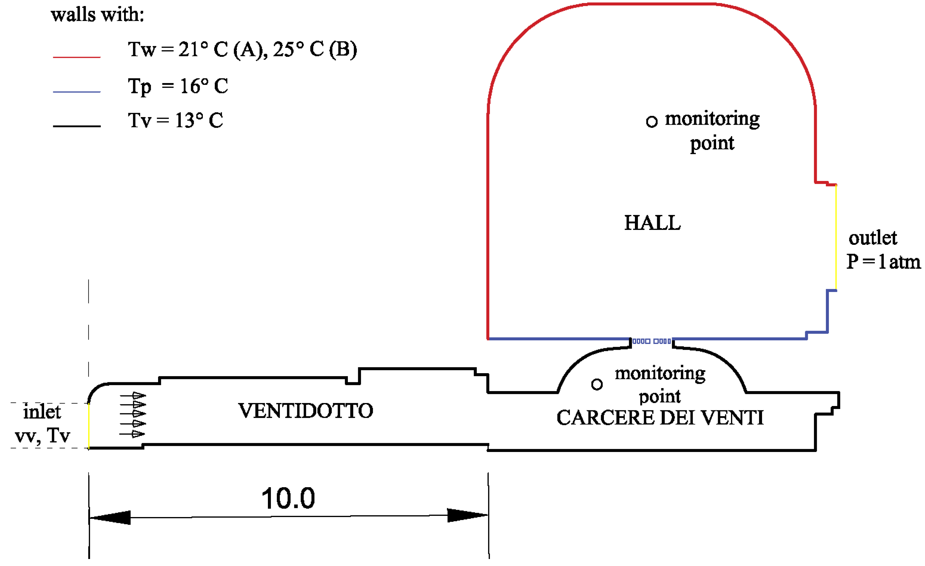In particular, two points controlling the velocity in the middle height of underground duct 10 m upstream of Villa Aeolia and 10 m upstream of villa Morlini Trento (for phase 1, see Figure 5); and two points, one in the cellar and one in the hall (for phase 2, see Figure 12).

3.1. Phase 1: The Global Cooling System

3.1.1. Studies, Geometry, and Mesh

Here, the configurations, geometry, mesh, and study cases of the whole cooling system are presented. First of all, it is important to explain another simplification of the geometric model: instead of representing all ventidotti (a, b, c) and villas (Villa Trento Carli, Villa Aeolia, and Villa Morlini Trento) in the same calculation domain, we separately represented the system that goes from Villa Trento Carli to Villa Aeolia and the one that goes from Villa Trento Carli to Villa Morlini Trento by neglecting the bifurcation of the ventidotto (a and b), as seen in Figure 5 [50]. This choice generated two independent studies:

• Studio Aeolia, analysing the cooling system of Villa Aeolia;
• Studio Morlini Trento, analysing the cooling system of Villa Morlini Trento.

The ventilation is governed by the altitude difference H. Its value was unknown since we did not have sufficient accurate speleological reliefs. So, for each study, we created four geometric models, one for each altitude ($H=65$ m, 75 m, 85 m, 95 m) chosen by following the topographic contour lines of the territory. We created an unstructured mesh composed of triangular elements. For example, for the geometry (Studio Aeolia, $H=85$ m) we had (10,550 elements, 779 boundary elements, grow rate 1.13, maximum element size 3.05 m). Its main characteristics are given in

Table 1. Characteristics of the Studio Aeolia mesh and of the Studio Morlini Trento mesh, according to height difference H. The maximum grow rate for both was 1.13 for the interior domain and 1.08 for the bounds.

		Studio Aeolia		Studio Morlini Trento
H [m]	Mesh	Maximum [m]	Minimum [m]	Maximum [m]	Minimum [m]
65	domain	2.35	0.0672	2.15	0.0305
	bound	0.874	0.0101	0.799	0.009
75	domain	2.7	0.0772	2.16	0.0309
	bound	1	0.0116	0.800	0.009
85	domain	3.05	0.0872	2.44	0.0349
	bound	1.13	0.0131	0.90	0.010
95	domain	3.4	0.0972	2.75	0.0389
	bound	1.26	0.0146	1.01	0.011

. Near the wall, a thicker quadrilateral mesh with five layers was generated, taking into account the viscous effects (boundary layer stretching factor 1.2). The grid independence test was performed for a finer mesh (27,779 elements, 1399 boundary elements, grow rate 1.1, the same boundary layer characteristic, maximum element size 2.72 m) and an extra-fine mesh (35,688 elements, maximum element size 0.651 m, grow rate 1.05, with the same boundary layer characteristic). The velocity of the monitoring point was compared at the end of the computation for the three meshes (mesh fine $v=2.41$ m/s, mesh finer $v=2.47$ m/s, mesh extra-fine $v=2.48$ m/s) in the case of $DT$ = 20 ${}^{°}$C. So, if we refer to the pivot case, the mesh extra-fine, we had a difference between the results of $2.8\%$ for the chosen mesh. We preferred to have this discrepancy, which remained very low, and a less-expensive time computational calculation.

For each model we determined the air velocity v in the ventidotti by varying the temperature difference $DT$. The simulations, identified by (Studio Aeolia, H, $DT$) and (Morlini Trento, H, $DT$), were performed for $H=65$ m, 75 m, 85 m, 95 m, and $DT=$ 5, 10, 15, 20 K. The temperature difference values $DT$ were chosen because they cover most of the system’s operating configurations in the summer period, from external temperatures $T_e=16$ ${}^{°}$C ($DT=5$ ${}^{°}$C) to temperatures of $T_e=31$ ${}^{°}$C ($DT=20$ ${}^{°}$C). For $T_e<5$ ${}^{°}$C, the system reversed its operation. In total, we had 32 CFD simulations.

3.1.2. Boundary Conditions

The characteristics of the fluid were set as: air temperature $T_i=11{}^{°}$C, reference pressure $P_{ref}=1$ atm. ${\rho }_0$ is the air density at a reference pressure $P_{ref}$ and at a temperature $T_0=(T_{ref}+DT)$. g is the acceleration due to gravity. $H=65,75,85,95$ m were the altitude difference between inlet and outlet. $DT=$ 5, 10, 15, 20 K. These values were used to assign the boundary conditions. The boundary conditions for the Studio Aeolia and the Studio Morlini Trento were as follows:

• Inlet condition on the cave opening: velocity coming in the inlet, pressure $P_{ref}$;
• Outlet condition on Villa Trento Carli opening at height $h_{TC}$: normal flow leaving the calculation domain with normal direction at the boundary and pressure $P=-g(H-h_{TC}){\rho }_0$, with $h_{TC}=18$ m;
• Outlet condition on the Villa Aeolia window of height $h_{Ae}$: normal flow leaving the calculation domain with normal direction on the boundary and pressure $P=-g(H-h_{Ae}){\rho }_0$ with $h_{Ae}=8$ m;
• Outlet condition on the Villa Morlini Trento window at height $h_{MT}$: normal flow leaving the calculation domain with normal direction on the boundary and pressure $P=-g(H-h_{MT}){\rho }_0$ with $h_{MT}=7$ m;
• Wall Functions applied to the wall boundaries (with the wall roughness $k_{eq}=0.03$ m);
• We considered a volume force in all the domain, taking into account the effect of gravity on the fluid, $F=-g{\rho }_i$ with ${\rho }_i$ the density of the air in the cave at the temperature $T_i$.

3.1.3. Results

The average air velocity (see

Table 2. (left) Studio Aeolia, (right) Studio Morlini Trento: average air velocity in the ventidotto to 10 m upstream of Villa Morlini Trento, depending on the altitude difference H and the temperature difference $DT$.

H [m]	DT [K]	v [m/s]
65	5	−0.74
65	10	0.004
65	15	0.76
65	20	1.77
75	5	−0.5
75	10	0.91
75	15	1.61
75	20	2.07
85	5	−0.19
85	10	1.10
85	15	1.66
85	20	2.12
95	5	−0.14
95	10	1.14
95	15	1.83
95	20	2.34
85	5	−0.08
85	10	0.03
85	15	0.18
85	20	0.30
95	5	0.60
95	10	0.085
95	15	0.24
95	20	0.39

) was calculated in the section located in the ventidotto at 10 m upstream of Villa Aeolia (in Studio Aeolia) and at 10 m upstream of Villa Morlini Trento (in Studio Morlini Trento), as indicated by the position of the red dot in Figure 5. We checked and then used the values of the velocity computed in the ventidotto at 10 m upstream of the villas, since we needed the averaged air velocity in the ventidotto, not affected by the local aerodynamics effects of the villas. Then, in phase B, we used these values. Some visualisations of results are shown in Figure 6 and Figure 7. In the cave, there can be a strong variation of speed, especially in very narrow passage areas. In fact, the air velocity increases next to the inlet (9 m/s) and in the ventidotti near the villas (3 m/s).

By observing the numerical results, we can affirm that:

• The height of the cave opening is $H>65$ m. The results of the Studio Aeolia showed that when $H=65$ m and 5 K $<DT<10$ K the flow was reversed (the velocities had negative values). For the other cases ($H=75,85,95$ m), the velocities had positive value.
• By observing the results of the Studio Morlini Trento with $H<85$ m, the system did not work because the pressure drops were too high. In fact, the ventidotto is 135 m longer than the one that feeds Villa Aeolia and the two villas are located at about the same altitude (Villa Aeolia is at 8 m and Villa Morlini Trento at 7 m above the ground). It follows that the height of the inlet is $H\ge 85$ m.
• By comparing the results of Studio Aeolia and Studio Morlini Trento for $H=85$, 95 m, we noticed that for Studio Morlini Trento the velocities were much lower (of a factor between 6 and 14 depending on the $DT$). It follows that the ventidotto (c) (which reaches Villa Morlini Trento) should not be as efficient as ventidotto (b and a). Many men of letters of the past spoke of Villa Aeolia and not of Villa Morlini Trento, praising the cooling system. Perhaps the system of Villa Morlini Trento was built after that of Villa Aeolia, trying to have the same cooling effect. However, the technicians of the past did not consider the great flow losses that were associated with the length of the ventidotto, and they obtained velocities (and consequently the air flow) much lower than those attended in the cellar of Villa Aeolia, called “Carcere dei Venti”.
• In the Studio Morlini Trento and Studio Aeolia, the cooling system worked for $H=95$ m, even in presence of a weak thermal difference ($DT=5$ K). In addition, for $H=95$ m, the air velocity average in the ventidotto of Villa Aeolia was quite close to the experimental data.

The model that best fit the real system was for $H=95$ and $H=85$. These velocity laws were used to study the fluid dynamic behaviour of Villa Aeolia.

3.1.4. Validation Case

We validated the simulation results in three steps, first controlling the mass balance, then comparing the numerical results with the analytical results and finally comparing with the experimental data of the two past experimental campaigns.

To verify the convergence of the simulation, we controlled that the mass imbalance between inlet and outlet of the computation of the phase 1 was less then 1%. Then, we compared the numerical results with the analytical solution by applying Equation (2) at the Studio Aeolia, but by considering only this villa and neglecting Villa Trento Carli (we performed the CFD simulation, changing the boundary condition on the opening of Villa Trento Carli by assigning a wall condition).

So, the airflow rate computed with Equation (2) was $m_1=18.02$ m${}^2$/s (the unit of measure takes into consideration a two-dimensional field), with $C_D=0.61$ m, ${\rho }_i=1.24$ kg/m${}^3$, ${\rho }_e=1.16$ kg/m${}^3$ ($T_e=304.55$ K, $DT=20$ K), $h_2=95$ m, $h_1=8$ m, and the Villa Aeolia opening $A_1=2.25$ m${}^2$. The airflow computation fit well with the numerical results: for the Studio Aeolia when $H=95$ m, the airflow through the opening of Villa Aeolia was 12 m${}^2$/s and the flow through the Villa Trento Carli opening was 7.2 m${}^2$/s. Their sum approached the value of the analytical solution considering the presence of only Villa Aeolia.

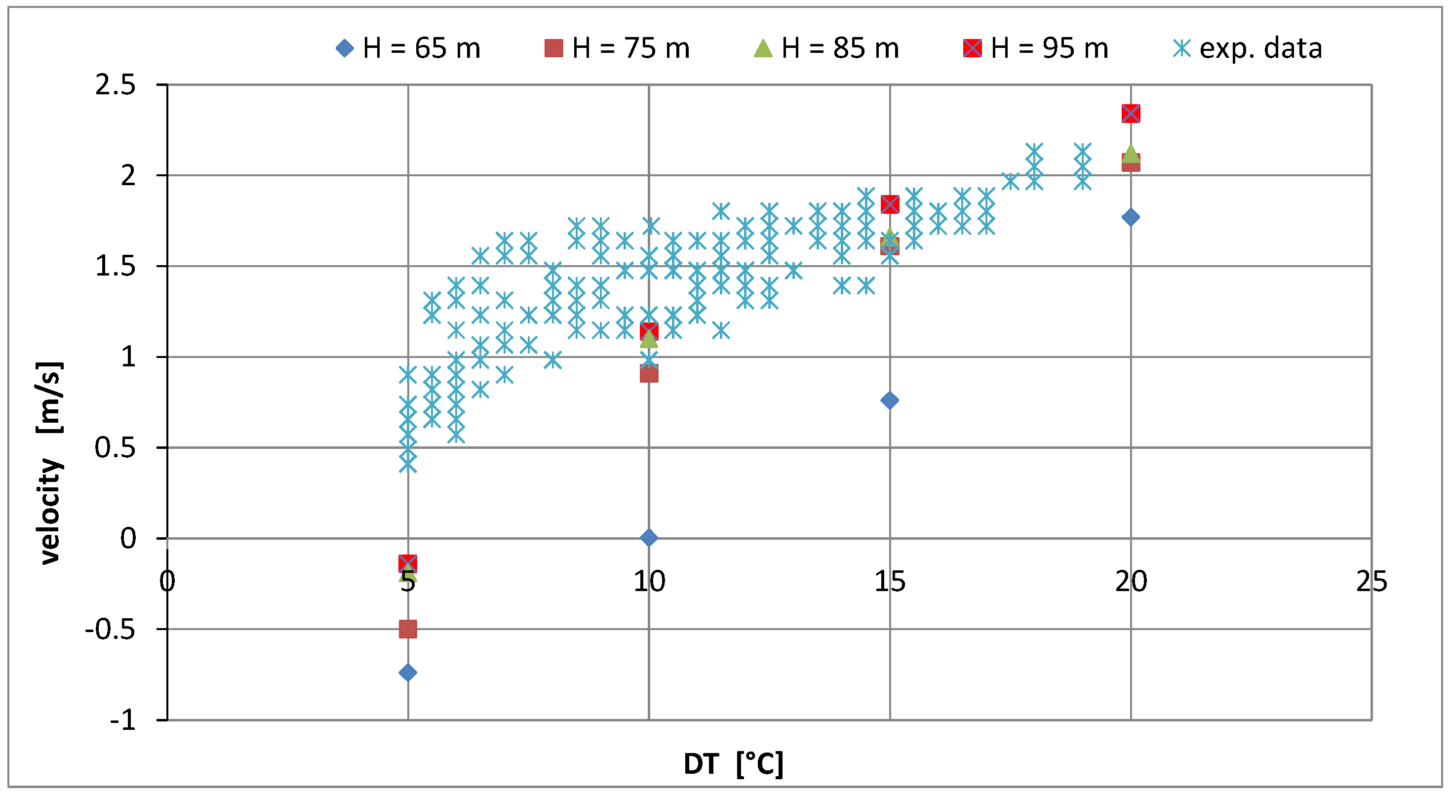
Then, we used the past experimental data to calibrate the model. In particular, [46] recorded during the period between June and November 1980 the air velocity, indoor temperature, and the outdoor temperature in the cooling system of Costozza. Their measurement campaign was particularly realised in the ventidotto (a) and (b), in Covolo Carli, and in Villa Aeolia: in the cellar, in the hall, and in the rooms next to the hall (not modelled here). Punctual measures were also carried out in the other villas affected by the cooling system. So, we used their recordings to validate our model. In detail, we used the measures (velocity and temperature difference $DT$) recorded in the Villa Aeolia across the access door of the cellar, the Carcere dei Venti. We chose to use these data, since they were the most complete. To have a suitable comparison with our velocity results in the ventidotto, we applied a discharge coefficient $Cd=1/0.61$ to these experimental data. This value was chosen from existing values for rectangular large openings in accordance with [53,54] to simulate the passage across the door). The comparison is shown in the graphic of Figure 8. Our results fit the data well, but they slightly overestimated the values for elevated $DT$.

A similar comparison was made with the experimental determinations obtained by [48] in 1990. The comparison is shown in Figure 9. These measurements were located at approximately 30 m upstream of Villa Aeolia and give the maximum air velocity incoming in the Carcere dei Venti only through ventidotto (a). In fact, during these measurements, ventidotti (b), (c), and the Covoletto Carli were closed to maximise the airflow in ventidotto (a), neglecting the presence of Villa Trento Carli. To compare our model with these mesurements, we performed new simulations (by using exactly the same model and configuration of Studio Aeolia), but applying a wall condition on the Villa Trento Carli opening (by removing the previous outlet condition). In this way, we maximised the airflow rate, as done in the experimental determinations. Finally, we compared the air velocity (depending on $DT$) at 30 m upstream to Villa Aeolia with the data. By considering the difference between the values of the two experimental campaigns and the small discrepancies with our model, which fit the system very well for $10{}^{°}\mathrm{C}\le DT\le 15{}^{°}\mathrm{C}$, we can affirm that the model is representative of the real phenomenon.

3.2. Phase 2: Villa Aeolia

After the development of the model of the cooling system, the specific cooling system of Villa Aeolia, on a larger scale, was studied with 2D CFD simulations. The data obtained from the macroscopic analysis were used as input. In particular, we used the air velocity law (depending on the outdoor temperature $T_e$ or $DT$) determined by the previous simulations to study the effect of the cooling in the main hall of Villa Aeolia.

3.2.1. Geometry and Mesh

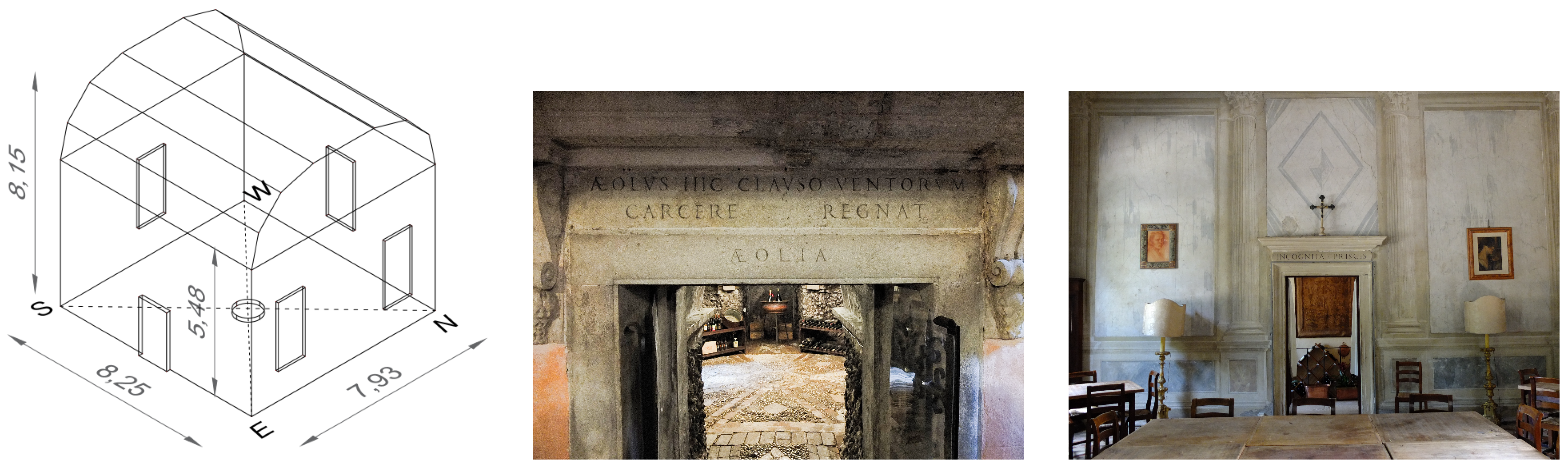
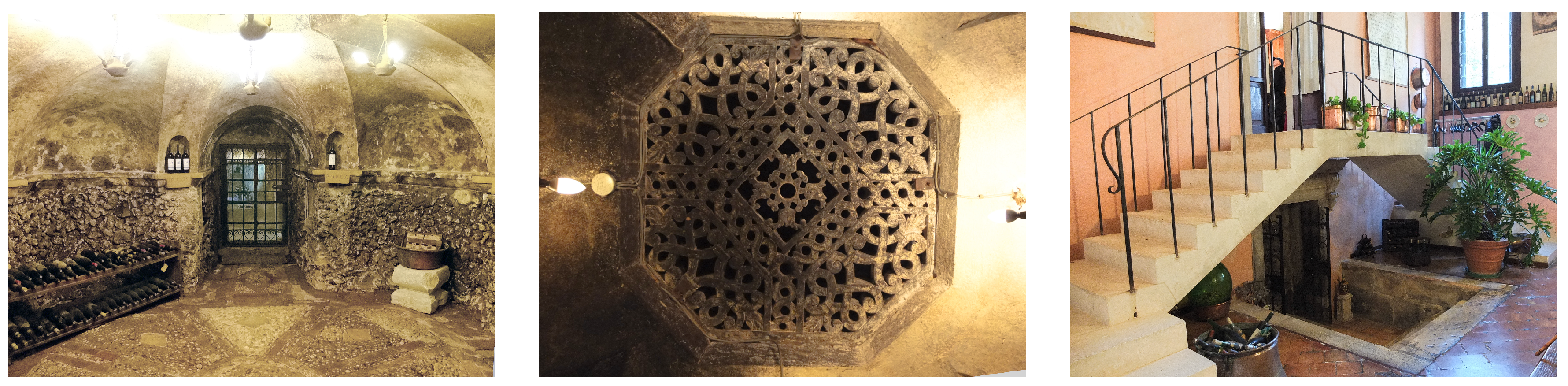
Villa Aeolia is a small pavilion with a square plan composed of a room (interior size in plan 8 m × 8 m and height of the roof 8 m) named Apollinea hall, and a cellar (Carcere dei Venti). The ventidotto (a), connected on the north-east wall of the cellar, takes the cooled airflow in the Carcere dei Venti. Thanks to a marble grating situated on the ceiling of the cellar (or pavement of the hall), the air flows to the Apollinea hall. Figure 10 and Figure 11 show the curious interior of the villa, composed of a cellar and an elegant superposed hall.

2D CFD simulations were performed by representing the north-east south-west section of the villa passing through the centre of Apollinea hall. The geometric model is shown in Figure 12, with the boundary conditions explained in the section below.

We created an unstructured mesh composed of triangular elements: 11,538 domain elements, 577 boundary elements, grow rate 1.15, maximum element size 0.51 m, minimum element 0.227 m. For the bounds the grow rate was 1.08, the maximum element 0.14 m, and the minimum element 0.00163 m. On the wall-type elements, a thicker quadrilateral mesh was refined to account for the viscous effects (the total thickness of the boundary layer was 0.10 m, divided in nine layers with a stretching factor of 1.15).

The grid independence test was performed for this mesh, a finer mesh (15,845 elements, maximum element size 0.33 m, grow rate 1.08, with the same boundary layer characteristic), and a coarser mesh (8369 elements, maximum element size 0.76 m, grow rate 1.2, with the same boundary layer characteristic). The velocity and temperature values of the monitoring point were compared at the end of the computation for the three meshes (coarse mesh $v=0.3475$ m/s $T=295.19$ K, chosen mesh $v=0.3153$ m/s $T=295.11$ K, fine mesh $v=0.32$ m/s $T=295.324$ K). So, if we refer to a pivot case, the finer mesh, we had a difference between the velocity results of $1.15\%$ and for the temperature a difference of $10.042\%$.

3.2.2. Boundary Conditions

In the model we assigned to bounds one condition of the inlet that takes the airflow in the ventidotto, one of the outlet, representing the access door to the hall; and wall-type conditions, having a different temperature as a function of the position (walls of the ventidotto $T_v$, of the pavement $T_p$, of the exterior walls $T_w$). In this scheme we did not consider the presence of the windows in the hall. On the other hand, the experimental data by [46] were recorded with the windows closed. The opening has vertical dimensions equal to the height of the door in the room. In order to assign the boundary conditions, we referred to past experimental measurements. On the opening is set the condition of outlet with a reference pressure of 1 atm for the CFD equations and an outflow condition for the heat equations. We performed two study cases (A, B), for two external temperatures $T_e$ = 21 ${}^{°}$C and $T_e$ = 31 ${}^{°}$C corresponding to $DT$ = 10 ${}^{°}$C and $DT$ = 20 ${}^{°}$C. As proved in the simulations of phase 1, in these conditions the air velocity $v_v$ changed. In particular, the air velocity in the ventidotto was 1.12 m/s for $DT$ = 10 ${}^{°}$C ($v_v=(1.14+1.10)/2=2.23$ m/s) and 2.23 m/s for $DT$ = 20 ${}^{°}$C ($v_v=(2.34+2.12)/2$ = 2.23 m/s). This value is calculated by using the previous results, by choosing the velocity values averaged for the altitude $H=$ 85 m and 95 m. The air temperature in the ventidotto $T_v$ was set 13 ${}^{°}$C (this temperature is slightly higher than the cave’s air temperature 11 ${}^{°}$C, but this value was set to past recordings close to Carcere dei Venti). This temperature was also assigned to the walls of the cellar and of the ventidotto. The temperature of the slab of the hall was set to $T_p$ = 16 ${}^{°}$C, considering that this was the average temperature in the hall when the cooling system was activated [46]. The temperature of the exterior walls of the hall was set in case A ($T_e$ = 21 ${}^{°}$C) to 21 ${}^{°}$C. This value was chosen because it was the average temperature in the hall when the cooling system was closed for a day with an average daily temperature of 25 ${}^{°}$C. For case B ($T_e$ = 31 ${}^{°}$C), the temperature of the exterior walls of the hall was set to 25 ${}^{°}$C.

A summary of the conditions is given in

Table 3. Boundary conditions for cases A and B.

	Case A	Case B
$T_e$	21 ${}^{°}$C	31 ${}^{°}$C
$DT$	10 ${}^{°}$C	20 ${}^{°}$C
inlet	V${}_v$ = 1.12 m/s	V${}_v$ = 2.23 ${}^{°}$C
	T${}_v$ = 13 ${}^{°}$C	T${}_v$ = 13 ${}^{°}$C
outlet	$P=1$ atm	$P=1$ atm
wall ventidotto	T${}_v$ = 13 ${}^{°}$C	T${}_v$ = 13 ${}^{°}$C
wall pavement	T${}_p$ = 16 ${}^{°}$C	T${}_p$ = 16 ${}^{°}$C
wall hall	T${}_w$ = 21 ${}^{°}$C	T${}_w$ = 25 ${}^{°}$C

.

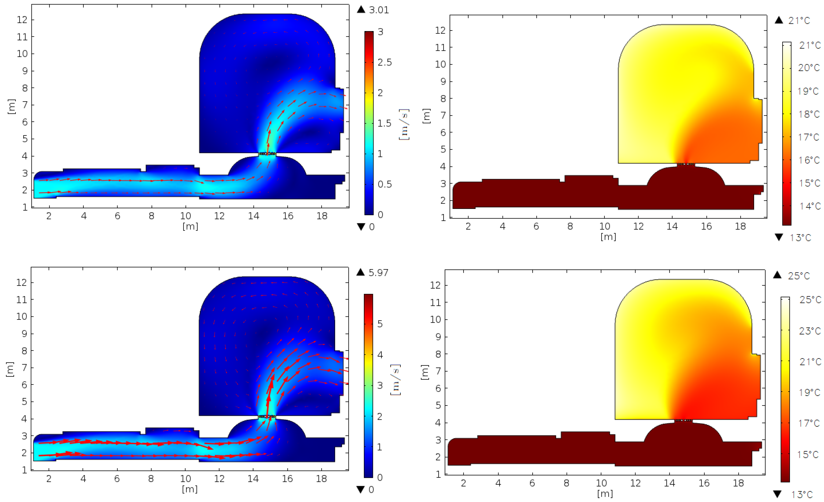
3.2.3. Discussion

The average temperature in the room was 17.5 ${}^{°}$C for an inlet velocity of 1.12 m/s and $T_{ext}$ = 25 ${}^{°}$C. When the walls had a temperature of 25 ${}^{°}$C for a maximum external temperature of ${31}^{°}$C, the average temperature in the hall did not exceed 20 ${}^{°}$C (18.93 ${}^{°}$C ), see

Table 4. Results of case studies A and B.

Case in the Hall	Inlet Velocity	Average Temperature
A	1.12 m/s	$17.86$${}^{°}$C
B	2.23 m/s	$18.93$${}^{°}$C

. The flow coming from the ventidotto goes through the marble grid, and then a part goes to the door and the rest reaches the ceiling and then falls back to the wall. Therefore, the area of the hall that is located between the marble grid and the door is the coldest and most uncomfortable: for case A $0.5$ m/s $\le v\le$ 1 m/s and the average temperature was 16.5 ${}^{°}$C, for case B $0.5$ m/s $\le v\le$ 2 m/s and the average temperature was 16 ${}^{°}$C. In other areas of the hall, instead the air velocity and the temperature remained moderate: for case A $0.0$ m/s $\le v\le$ 0.5 m/s and the temperature was 18 ${}^{°}$C $\le T\le$ 21 ${}^{°}$C, for case B $0.0$ m/s $\le v\le$ 1 m/s and temperature 21 ${}^{°}\mathrm{C}\le T\le$ 25 ${}^{°}$C. It is interesting to note how the temperature distribution relates to the flow field, and it was extremely low even on the hottest days (see Figure 13).

It follows that a 3D simulation is necessary to know the spatial thermo-hygrometric conditions, even if the average values of the study are similar to those determined experimentally in the past recordings.

From the perspective of re-establishing the cooling system in other buildings in the area of Costozza and in the other villas, the same type of modelling can be used. In fact, the simplified model gives us some general indications of the thermo-hygrometric conditions in the rooms of the villas with low computational cost.

3.2.4. Validation

A control of the mass imbalance was done. There was a difference of $1.23\%$ between the inflow rate $1.22$ m${}^2$/s and the outflow $1.235$ m${}^2$/s for case A. For case B, the inflow rate was $2.43$ m${}^2$/s and the outflow $2.45$ m${}^2$/s with a difference of $0.82\%$. The results were checked again with experimental data of [46] that recorded an average temperature during a summer day in the hall of around 16–17 ${}^{°}$C with the cooling system activated. It was not described if the windows were opened during the measurement. However, it is certain that the access door to the hall was opened. All these controls reassure us about the good quality of our results.

4. Conclusions

On-site experimental campaigns can provide a lot of data on ventilation flow rates, average velocity in the ventidotti, and the distribution of temperature flows, but they are very expensive and time-consuming. This is proved by the fact that in 38 years only two experimental campaigns have been carried out on such a fascinating ventilation system. The macroscopic model of the geothermal cooling system, despite the strong simplification, can provide a reproduction of the cooling system with good precision, not only for the analysed villa, but also for the other villas and buildings connected to the ventidotti.

Although it is based on a simplified model of the geothermal cooling system, the macroscopic analysis of the ventidotti is representative of the real phenomenon, as shown by the comparison with the experimental data. This can be used to simulate the passive cooling in villas of Costozza as developed here for Villa Aeolia.

The ventidotto can provide fresh airflow rates that cool the walls of the room and maintain the temperature below 20 ${}^{°}$C even on hot summer days. An advantage is that the system works in a self-adaptive way, the airflow increases when the outdoor temperature increases. This self-adjustment allows us to compare the cooling system to a modern environmental control system. This self-adjustment allows us to compare the cooling system to modern air conditioning.

The cooling system proves to be a work of civil engineering that thanks to its extension and capillarity in the soil of Costozza could be reused to cool many buildings. The system could be put back into operation with little action, by inserting adjustable grids to vary the air flow rates coupled to a dehumidification system. This example highlights the potential to plan together with local climatic elements and the territory.

The design of the villas of Costozza, which we can define as bioclimatic, has been almost neglected until this day, even though it is part of Italian cultural and historical heritage. In fact, the effectiveness of the passive cooling system was already known to Palladio [40] and Scamozzi [41].

Over the years, this technological wealth has not been studied. This subject opens the research to other historical and technological tracks that highlight the importance of the natural ventilation system in Costozza villas for the architects of the past that we can define as “bioclimatic architects”.