A Bi-Objective Vehicle-Routing Problem with Soft Time Windows and Multiple Depots to Minimize the Total Energy Consumption and Customer Dissatisfaction

Abstract

In recent years, the impact of the energy crisis and environment pollution on quality of life has forced industry to actively participate in the development of a sustainable society. Simultaneously, customer satisfaction improvement has always been a goal of businesses. It is recognized that efficient technologies and advanced methods can help transportation companies find a better balance between progress in energy saving and customer satisfaction. This paper investigates a bi-objective vehicle-routing problem with soft time windows and multiple depots, which aims to simultaneously minimize total energy consumption and customer dissatisfaction. To address the problem, we first develop mixed-integer programming. Then, an augmented $ϵ$-constraint method is adopted to obtain the optimal Pareto front for small problems. It is very time consuming for the augmented $ϵ$-constraint method to precisely solve even medium-sized problems. For medium- and large-sized problems, two Non-dominated Sorting Genetic Algorithm-II (NSGA-II)-based heuristics with different rules for generating initial solutions and offspring are designed. The performance of the proposed methods is evaluated by 100 randomly generated instances. Computational results show that the second NSGA-II-based heuristic is highly effective in finding approximate non-dominated solutions for small-size and medium-size instances, and the first one is performs better for the large-size instances.

1. Introduction

The vehicle-routing problem (VRP) is a NP-hard combinatorial optimization problem (c.f. Laporte [1]; Jozefowiez et al. [2]; Laporte [3]). It focuses on finding a set of routes to serve customers. There has been significant research on VRP, which mainly includes capacitated VRP (c.f. Toth and Vigo [4]; Ralphs et al. [5]; Fukasawa et al. [6]), periodic VRP (c.f. Francis and Smilowitz [7]; Gulczynski [8]; Campbell and Wilson [9]), pickup and delivery problems (c.f. Berbeglia et al. [10]; Parragh et al. [11]), VRP with time windows (c.f. Tan et al. [12]; Br$\ddot{a}$ysy and Gendreau [13]; Tang et al. [14]), and multiple-depots VRP (c.f. Montoya-Torres et al. [15]).

The vehicle-routing problem with time windows (VRPTW) has been extensively studied in the context where high-performance industries hope their commodities and materials are delivered and picked up within an expected time window. Depending on the type of time window, VRPTW can be further distinguished into VRP with hard time windows (VRPHTW) and VRP with soft time windows (VRPSTW). For VRPHTW, a route is feasible only if every customer is served within the time window (c.f. Ho and Haugland [16], Alvarenga et al. [17], Dabia et al. [18], Desaulniers et al. [19]). VRPSTW can be considered as a relaxation of VRPHTW, which has valuable practical applications (Figliozzi [20]). For the VRPSTW, time window violation is permitted but with a penalty, i.e., early or/and late services will generate an extra cost. Liberatore et al. [21] propose a branch-and-price algorithm for the VRPSTW. Lu and Yu [22] study a pickup and delivery VRPSTW and combine data envelopment analysis with a genetic algorithm (GA). Duygu et al. [23] deal with a VRPSTW with stochastic travel times and develop a tabu search method for it. Iqbal et al. [24] propose a hybrid meta-heuristic combining artificial bee colony (ABC) algorithm for a multi-objective VRPSTW, in which the objectives are to minimize total traveling distance, number of time window violations and number of required vehicles. Kumar and Panneerselvam [25] give a comprehensive survey about the various exact methods and the heuristics and meta-heuristics used to solve the VRP and its variants, especially the VRPTW and the capacitated vehicle-routing problem (CVRP). For a more recently survey, Dixit et al. [26] review some of the recent advances in the VRPTW using meta-heuristic techniques, e.g., evolutionary and swarm intelligence-based algorithms such as Particle Swarm Optimization (PSO). The authors also highlighted the research gaps and prospects in this field.

In this work, we investigate a variant of the VRPTW with energy-saving consideration, to minimize total energy consumption and customer dissatisfaction (i.e., total violation of time windows). For small-size problems, the augmented $ϵ$-constraint method is adopted to obtain the exact Pareto fronts. Two NSGA-II-based heuristics are carefully designed to tackle medium- and large-size problems. Extensive computational experiments are conducted to evaluate and compare the performance of these two algorithms.

The objective of this study is to address the bi-objective VRP with soft time windows and multiple depots from the perspectives of the construction of mathematical formulation and the design of heuristic algorithms. There are three tasks in this study, which are: (1) construct a mixed-integer linear programming model to describe the investigated problem comprehensively; (2) design a detailed procedure of the heuristic algorithms to obtain good Pareto fronts quickly; and (3) conduct the computational experiments to evaluate and validate the performance of the proposed algorithms. The main contribution of this paper is threefold:

(1)

We first consider bi-objective optimization for the energy minimization VRP with soft time windows and multiple depots.

(2)

A novel mixed-integer programming model is formulated.

(3)

An augmented $ϵ$-constraint method is adopted to obtain the optimal Pareto solutions for small-size instances. In addition, two NSGA-II-based heuristics are designed to efficiently solve medium- and large-size instances.

The remainder of the paper is organized as follows. Section 2 reviews the related literature. Section 3 presents the description of the problem and proposes a mixed-integer programming formulation. Section 4 gives details of the augmented $ϵ$-constraint method and two NSGA-II-based heuristics. Computational results on numerous instances are reported in Section 5. Conclusions and future research directions are suggested in Section 6.

2. Literature Review

Multiple depots and the energy-saving consideration are considered to be important characteristics for the investigated problem. To be more focused, we will only review the most relevant literature bellow.

In practice, there may be many depots for vehicles to depart from. Consequently, multiple-depots VRP has been investigated by many researchers. Cordeau et al. [27] investigated multiple-depots VRP with time windows (MDVRPTW) and develop a hybrid tabu search heuristic to minimize the number of vehicles. Dondo and Cerdá [28] studied the MDVRPTW with a fleet of heterogeneous vehicles. They provided a mixed-integer linear programming, and proposed a three-phase cluster-based algorithm. Goela and Gruhn [29] studied a MDVRPTW with heterogeneous vehicle fleets and pickup and delivery orders. They proposed a large neighborhood search to maximize the transportation profit. Flisberg et al. [30] considered a multi-period MDVRPTW with split pickup and delivery, and a heterogeneous truck fleet. A linear programming and tabu search algorithm is proposed. Bettinelli et al. [31] developed a branch-and-cut-and-price algorithm for MDVRPTW with heterogeneous vehicles to minimize the total costs. Luo and Chen [32] proposed an improved shuffled leapfrogging algorithm for MDVRPTW to minimize the total costs. There has been several pieces of research focusing on multi-objective MDVRPTW. Tan et al. [33] provided an evolutionary algorithm for a multi-objective MDVRPTW, which aims at minimizing total distances and number of vehicles. Ghoseiri and Ghannadpour [34] developed a GA for MDVRPTW to minimize the number of vehicles and total distances. Karakati$\check{c}$ and Podgorelec [35] focused on the MDVRP. A detailed survey of GAs designed for solving MDVRP was presented. The results of a thorough experiment are presented and discussed, which evaluate the efficiency of different existing genetic methods on standard benchmark problems. The insights into strengths and weaknesses of specific methods, operators and settings are presented. The above multi-depot VRP (MDVRP) research mainly focused on the improvement of transportation efficiency and effectiveness at minimizing travel costs or distances, but energy saving and environment concern have not been considered.

The following researches take the energy consumption and/or customer satisfaction into consideration. Hassanzadeh and Rasti-Barzoki [36] proposed a new bi-objective mathematical model to reduce the consumption of energy and decrease the tardiness penalty in supply chain scheduling and the VRP. A new Non-dominated Sorting Genetic Algorithm based on shaking and local search strategies of the Variable Neighborhood Search algorithm was developed. The performance of the proposed algorithm was demonstrated by computational experiments.

Zhang et al. [37] considered an Electric Vehicle-Routing Problem (EVRP) to minimize the energy consumption of electric vehicles. The corresponding mathematical model is formulated. An ant colony (AC) algorithm-based meta-heuristics is proposed as the solution method of the problem. The benefits of using an energy consumption-minimizing objective function rather than a distance-related one is also illustrated.

Ghannadpour and Zarrabi [38] presented a new model and solution for the multi-objective heterogeneous vehicle-routing and scheduling problem. A new mathematical formulation for the VRPTW is also presented using the proposed concept of heterogeneities. The customers’ priority for servicing is considered.

Abad et al. [39] proposed a bi-objective model for the pickup and delivery pollution-routing problem with integration and consolidation shipments in cross-docking system, to minimize total system cost, and total fuel consumption by vehicles. Three multi-objective meta-heuristic algorithms are proposed to solve this problem.

Androutsopoulos and Zografos [40] formulated and solved a bi-objective, time, load, and path-dependent vehicle-routing problem with time windows (BTL-VRPTW). The need to address simultaneous routing and path-finding decisions is considered to be a key feature. A generic solution framework is proposed to address this problem.

Recently, the trend of sustainable development has gained increased attention as a near-future business driver. Many researchers are focused on sustainable production, sustainable transportation, etc. Demartini et al. [41] introduced a Manufacturing Value Modeling Methodology (MVMM), and sustainability is investigated as a performance dimension when applying the MVMM. In their follow-up study, Demartini et al. [42] used the MVMM as a value-mapping framework to help firms in creating value propositions better suited for sustainability considering economic, environmental and social perspectives. Concerning sustainability, the setting of a catalogue that presents an overview of sustainable external and internal impact factors is constructed. A mapping between them that translates business goals into manufacturing strategy is provided. The operational performance is improved by adopting a set of sustainable industrial practices.

On the other hand, energy and environment problems have been gaining increased attention in the sustainable development context. Various variants of VRP that consider energy consumption and greenhouse gas emissions are beginning to be studied, such as Energy Minimization VRP (EMVRP) (c.f. Kara et al. [43]; Fukasawa et al. [44]), Pollution-Routing Problem (PRP) (c.f. Bektaş and Laporte [45]; Demir et al. [46]) and Green VRP (GVRP) (c.f. Erdoǧan and Miller-Hooks [47]; Lin et al. [48]). Single depot EMVRP is first introduced in Kara et al. [43]. They first defined arc cost as the product of vehicle weight and arc length and assume that the vehicles types, vehicle speed, air condition, and road condition are constant. Xiao et al. [49] proposed a simulated annealing heuristic for the EMVRP. The problem was further studied by Fukasawa et al. [44], and two formulations and a branch-and-cut algorithm are proposed. Liu et al. [50] investigated a VRP with alternative paths. The objective is also related to energy consumption, i.e., finding a route with minimal carbon footprint. The time-dependent heterogeneous-fleet vehicle is considered. A GA is designed to solve this problem. The experimental results show that the alternative path has a significant impact in terms of carbon footprint. However, in existing works, MDVRPTW with energy minimization has not been investigated.

In real applications, energy-saving and customer satisfaction are often incompatible, but a better balance between the two objectives should be achieved by efficient optimal models and methods. Little research can be found in the literature. Demir et al. [46] investigated a bi-objective PRP with single depot focusing on simultaneously minimizing the fuel consumption and total driving time. An adaptive large-neighborhood search algorithm was proposed. To the best of our knowledge, bi-objective EMVRP with soft time windows and multiple depots has not been studied.

3. Problem Description and Formulation

In this section, the problem is described in detail. Then, a mixed-integer linear programming is proposed to represent the investigated problem comprehensively.

EMVRP is defined on a complete graph $G=(V,A)$ with $V=N_0\cup N_1$, where A, $N_0$ and $N_1$ denote the set of arcs, the set of depots and the set of customer locations, respectively. Let $d_{ij}$ denote the distance between vertex i and j, and $d_{ij}=d_{ji}$. $K=\{1,2,\dots ,|K\left|\right\}$ represents the fleet of heterogeneous vehicles located at $N_0$, and vehicle k has the curb weight $w_k$ and the capacity $V_k$. A desired pickup time window of customer $i\in N_1$ is denoted by $[e_i,l_i]$. The vehicle must wait until $e_i$ to start the service if it arrives early. The customer will be dissatisfied if the service starts late, and the dissatisfaction is measured by $max\{0,a_{ik}-l_i\}$, where $a_{ik}$ denotes the arrival time of vehicle k at customer i. In this paper, we assume that the traffic condition and the speed of the vehicles are constant. The problem consists of determining a set of routes for vehicles such that (i) each customer is served exactly by a single vehicle; (ii) each vehicle starts from its departure depot with its curb weight $w_k$, and picks up $q_i$ when it visits customer i. The total load carried by any vehicle does not exceed its capacity $V_k$; and (iii) the departure depot of each vehicle is preset, and the arrival depots of vehicles should be optimized.

In this paper, energy consumption on an arc is computed by multiplying the length of arc and the total weight of the vehicle, as in Kara et al. [43] and Fukasawa et al. [44]. The customer dissatisfaction is defined as the total tardiness of vehicles (${\sum }_{i\in N_1}{\sum }_{k\in K}max\{0,a_{ik}-l_i\}$).

In the following, we give parameters and decision variables definitions. Then a novel bi-objective mixed-integer linear programming for the EMVRP is formulated. Since the investigated problem can be reduced to the VRP, which is NP-hard, then the investigated problem is also NP-hard.

3.1. Notation

Indices:

$i,j$:

index of points, including depots and customers, $i\ne j$.

k:

index of vehicles, {$k=1,\dots ,\left|K\right|$}.

Parameters:

$|N_0|$:

number of departure and arrival depots.

$|N_1|$:

number of customers.

$\left|K\right|$:

number of vehicles.

${\alpha }_{ik}$:

equal to 1 if depot $i\in N_0$ is set to be the departure depot of vehicle $k\in K$, 0 otherwise.

$d_{ij}$:

the distance between two vertexes i and j, $i,j\in N_0\cup N_1,i\ne j$.

$e_i$:

the earliest pickup time at customer i, $i\in N_1$.

$l_i$:

the latest pickup time at customer i, $i\in N_1$.

$q_i$:

pickup quantity at customer i, $i\in N_1$.

$s_i$:

service time at customer i, $i\in N_1$.

$w_k$:

curb weight of vehicle k, $k\in K$.

$V_k$:

load capacity of vehicle k, $k\in K$.

v:

the average speed of vehicles.

M:

a large enough number.

Variables:

$x_{ij}^k$:

equal to 1 if vehicle k passes arc $(i,j)$, 0 otherwise, $i,j\in N_0\cup N_1$ and $k\in K$.

$z_{ik}$:

equal to 1 if vehicle k visits vertex i, 0 otherwise, $i\in N_0\cup N_1$ and $k\in K$.

$a_{ik}$:

the arrival time of vehicle k at vertex i, $i\in N_1$ and $k\in K$.

$L_{ik}$:

tardiness of vehicle k at vertex i, $L_i^k=max\{0,a_i^k-l_i\}$, $i\in N_1$ and $k\in K$.

$Q_{ik}$:

total load of vehicle k before it loads at vertex i, $i\in N_0\cup N_1$ and $k\in K$.

$R_{ik}$:

the cumulative energy consumption of vehicle k at vertex i, $i\in N_0\cup N_1$ and $k\in K$.

3.2. The Formulation of the EMVRP

The formulation is as follows:

$$\begin{array}{c}\hfill min{f}_1=\sum _{k\in K}\sum _{i\in N_0}{R}_{ik}\end{array}$$

(1)

$$\begin{array}{c}\hfill min{f}_2=\sum _{k\in K}\sum _{i\in N_1}{L}_{ik}\end{array}$$

(2)

Objective function $f_1$ is to minimize the total energy consumption, $f_2$ aims to minimize the customer dissatisfaction.

$$\begin{array}{c}\hfill \mathrm{s}.\mathrm{t}.\sum _{k\in K}{z}_{ik}=1,i\in N_1\end{array}$$

(3)

$$\begin{array}{c}\hfill \sum _{j\in N_0\cup N_1,j\ne i}{x}_{ij}^k=z_{ik},i\in N_1,k\in K\end{array}$$

(4)

$$\begin{array}{c}\hfill \sum _{i\in N_0\cup N_1,i\ne j}{x}_{ij}^k=z_{jk},j\in N_1,k\in K\end{array}$$

(5)

Constraint (3)–(5) ensures that each customer is served exactly once by a vehicle.

$$\begin{array}{c}\hfill x_{ij}^k=0,i,j\in N_0,k\in K,i\ne j\end{array}$$

(6)

Constraint (6) ensures that vehicles do not travel between departure and arrival depots.

$$\begin{array}{c}\hfill \sum _{i\in N_1}{x}_{ij}^k=z_{jk},j\in N_0,k\in K\end{array}$$

(7)

Constraint (7) ensures that each vehicle returns back to a depot after serving customers.

$$\begin{array}{c}\hfill \sum _{j\in N_1}{x}_{ij}^k\le {\alpha }_{ik},i\in N_0,k\in K\end{array}$$

(8)

Constraint (8) ensures that vehicle k starts from its departure depot.

$$\begin{array}{c}\hfill \sum _{i\in N_1}{q}_i{z}_{ik}\le V_k,k\in K\end{array}$$

(9)

Constraint (9) ensures that the total load of vehicle k does not exceed its capacity $V_k$.

$$\begin{array}{c}\hfill Q_{jk}+(1-x_{ij}^k)M\ge w_k,i\in N_0,j\in N_1,k\in K\end{array}$$

(10)

$$\begin{array}{c}\hfill w_k+(1-x_{ij}^k)M\ge Q_{jk},i\in N_0,j\in N_1,k\in K\end{array}$$

(11)

Constraints (10) and (11) ensure that the load of vehicle k equals its curb weight $w_k$ when it departs from the depot.

$$\begin{array}{c}\hfill Q_{jk}+(1-x_{ij}^k)M\ge Q_{ik}+q_i,i\in N_1,j\in N_0\cup N_1,i\ne j,k\in K\end{array}$$

(12)

$$\begin{array}{c}\hfill Q_{ik}+q_i+(1-x_{ij}^k)M\ge Q_{jk},i\in N_1,j\in N_0\cup N_1,i\ne j,k\in K\end{array}$$

(13)

Constraints (12) and (13) detail the way of calculating the load carried by vehicle k before it loads at vertex i, which also can be used as subtour elimination.

$$\begin{array}{c}\hfill R_{jk}+(1-x_{ij}^k)M\ge Q_{jk}{d}_{ij},i\in N_0,j\in N_1,k\in K\end{array}$$

(14)

$$\begin{array}{c}\hfill R_{jk}+(1-x_{ij}^k)M\ge Q_{jk}{d}_{ij},i\in N_0,j\in N_1,k\in K\end{array}$$

(15)

$$\begin{array}{c}\hfill R_{jk}+(1-x_{ij}^k)M\ge R_{ik}+Q_{jk}{d}_{ij},i\in N_1,j\in N_0\cup N_1,i\ne j,k\in K\end{array}$$

(16)

$$\begin{array}{c}\hfill R_{ik}+Q_{jk}{d}_{ij}+(1-x_{ij}^k)M\ge R_{jk},i\in N_1,j\in N_0\cup N_1,i\ne j,k\in K\end{array}$$

(17)

Constraints (14)–(17) explain the calculation method of energy consumption of vehicle k before it loads at vertex i.

$$\begin{array}{c}\hfill a_{jk}+(1-x_{ij}^k)M\ge d_{ij}/v,i\in N_0,j\in N_1,k\in K\end{array}$$

(18)

$$\begin{array}{c}\hfill d_{ij}/v+(1-x_{ij}^k)M\ge a_{jk},i\in N_0,j\in N_1,k\in K\end{array}$$

(19)

$$\begin{array}{c}\hfill a_{jk}+(1-x_{ij}^k)M\ge a_{ik}+s_i+d_{ij}/v,i\in N_1,j\in N_0\cup N_1,i\ne j,k\in K\end{array}$$

(20)

$$\begin{array}{c}\hfill a_{jk}+(1-x_{ij}^k)M\ge e_i+s_i+d_{ij}/v,i\in N_1,j\in N_0\cup N_1,i\ne j,k\in K\end{array}$$

(21)

Constraints (18)–(21) calculates the arrival time of the vehicle k at each vertex.

$$\begin{array}{c}\hfill L_{ik}\ge a_{ik}-l_i,i\in N_1,k\in K\end{array}$$

(22)

$$\begin{array}{c}\hfill L_{ik}\ge 0,i\in N_1,k\in K\end{array}$$

(23)

Constraints (22) and (23) define the tardiness of vehicle k at vertex i.

$$\begin{array}{c}\hfill x_{ij}^k,z_{ik}\in \{0,1\},i,j\in N_0\cup N_1,i\ne j,k\in K\end{array}$$

(24)

$$\begin{array}{c}\hfill a_{ik},Q_{ik},R_{ik}\ge 0,i\in N_0\cup N_1,k\in K\end{array}$$

(25)

Constraints (24) and (25) are the restrictions on decision variables.

4. Solution Domain

There are various methods for solving multi-objective optimization problems, such as weighting method, $ϵ$-constraint method, evolutionary algorithms, etc. NSGA-II and $ϵ$-constraint method are known to be the most popular methods for bi-objective problems. In this section, we first describe bi-objective optimization and the principle of augmented $ϵ$-constraint method. Then, augmented $ϵ$-constraint method is adopted and two NSGA-II-based heuristics are designed.

4.1. Bi-Objective Optimization Problem

We consider the bi-objective optimization problem in the form as bellow, see Equations (26) and (27):

$$\begin{array}{c}\hfill \min \{f_1(\mathbf{x}),f_2(\mathbf{x})\}\end{array}$$

(26)

$$\begin{array}{c}\hfill \mathrm{s}.\mathrm{t}.\mathbf{x}\in \mathcal{X}\end{array}$$

(27)

where $f_1(\mathbf{x})$ and $f_2(\mathbf{x})$ denote total energy consumption and customer dissatisfaction respectively. Item $\mathbf{x}$ represents a decision variable vector, which belongs to the feasible solution region $\mathcal{X}$ defined by (3)–(25). A solution $\mathbf{x}$ is non-dominated only if it cannot be replaced by another solution which reduces one objective without increasing another (Tkindt and Ballaut [51]). A non-dominated solution is said to be Pareto-optimal, and the image of corresponding objective values of non-dominated solutions is called the Pareto front.

4.2. The Augmented $ϵ$-Constraint Method

The basic idea of $ϵ$-constraint method is to transform the bi-objective problem into a series of single-objective problems, which optimizes one objective with restricting another by a bound $ϵ$. The definition of the value of $ϵ$ in each iteration is one of critical factors for $ϵ$-constraint method. For our problem, the second objective is considered to be a constraint and restricted by $ϵ$. $[f_2^I,f_2^N]$, the range of $ϵ$, is obtained by following ideal point and nadir point (Bérubé et al. [52]).

-

Ideal point: ${\mathbf{f}}^I=(f_1^I,f_2^I)$, where $f_1^I=min\left\{f_1(\mathbf{x})\right\}$ and $f_2^I=min\left\{f_2(\mathbf{x})\right\}$, $\mathbf{x}\in \mathcal{X}$;

-

Nadir point: ${\mathbf{f}}^N=(f_1^N,f_2^N)$, where $f_1^N=min\{f_1(\mathbf{x}):f_2(\mathbf{x})=f_2^I\}$ and $f_2^N=min\{f_2(\mathbf{x}):f_1(\mathbf{x})=f_1^I\}$, $\mathbf{x}\in \mathcal{X}$;

Not all solutions obtained by the $ϵ$-constraint method are non-dominated (c.f. Ehrgott and Ruzika [53]). To avoid iterations that generate dominated solutions and accelerate the whole process, augmented $ϵ$-constraint method is proposed by Mavrotas [54], and further improved by Mavrotas and Florios [55]. It introduces a slack/surplus variable and a bypass coefficient. For our problem, we transform the original bi-objective problem into several single-objective problems, as shown in Equations (28)–(30):

$$\begin{array}{c}\hfill P^{\prime }(ϵ):\min \{f_1(\mathbf{x})-eps\times S\}\end{array}$$

(28)

$$\begin{array}{c}\hfill \mathrm{s}.\mathrm{t}.f_2(\mathbf{x})+S=ϵ\end{array}$$

(29)

$$\begin{array}{c}\hfill \mathbf{x}\in \mathcal{X}\end{array}$$

(30)

where

-

$eps$: a very small number, i.e., $eps={10}^{-5}$.

-

S: slack variable for $f_2$.

-

$ϵ$: $ϵ=f_2^N-i\times step$, where i denotes the iteration counter, and $step$ is the step size of $epsilon$ and set as the minimal unit value of $f_2$.

-

$\mathcal{X}$: the feasible region.

The value of $ϵ$ is also bounded by interval $[f_2^I,f_2^N]$. By varying the value of $ϵ$, a sequence of single-objective problems can be generated and solved. For each single-objective problem, $ϵ$-constraint is presented by an equality combining the slack variable S, $ϵ$ and $f_2$. To optimize the objective, $f_1$ is minimized and slack variable S is maximized with lower priority as its weight coefficient $eps$ is very small, forcing the program to obtain only non-dominated solutions (Mavrotas [54]).

As stated by Mavrotas and Florios [55], when slack variable S is larger than the $step$, then the same solution will be obtained with the slack variable being $S-step$ in the next iteration. Generation of no new non-dominated solutions makes the iteration redundant and therefore it can be skipped. Then a bypass coefficient b implying the number of consecutive iterations that can be skipped is introduced, which is calculated as the integer part of $(S/step)$. The framework of augmented $ϵ$-constraint method is shown in Algorithm 1.

Algorithm 1: The augmented $ϵ$-constraint method.

To obtain exact Pareto front is time consuming for the augmented $ϵ$-constraint method, even impossible for almost large-size NP-hard problems. In the next subsection, we focus on developing heuristics to find approximate Pareto front.

4.3. NSGA-II Based Heuristics

Non-dominated Sorting Genetic Algorithm-II (NSGA-II), proposed by Deb et al. [56], is a fast and elitist multi-objective evolutionary algorithm. NSGA-II starts with an initial set of solutions. During each generation, offspring solutions are reproduced by parent solutions using genetic operators. Then the population combining current solutions and offspring solutions is renewed. To be specific, the combined population is sorted by non-domination sort procedure into different ranks $\{F_1,F_2,\dots ,F_t,\dots \}$. Solutions of ranks in ascending order are sequentially added into the new population P, if $\left|P\right|+|F_{t-1}|\le pop$ and $\left|P\right|+|F_t|>pop$, the first $pop-\left|P\right|$ solutions in level $F_t$ are selected according to their crowding distances in descending order, where $pop$ denotes the predetermined population size. After the predefined number of generations is completed, a set of approximate Pareto solutions can be obtained.

In this section, two NSGA-II-based heuristics $H_1$ and $H_2$ with different rules of generating initial solutions and reproducing offspring are designed for our problem. The proposed heuristics are composed of (1) solution representation; (2) evaluation and feasibility check; (3) population initialization; (4) selection; (5) genetic operators; and (6) recombination.

To differentiate the two algorithms, the following statements should be noticed. $H_1$ focuses on constructing routing for each vehicle based on the customer sequence, while $H_2$ searches for available vehicles for each customer. Besides, the initialization procedure of two algorithms are various, as shown in Algorithms 2 and 3. Although these two algorithms share the same mutation operator 1, $H_1$ adopted a different crossover operator and a different mutation operator 2 compared to $H_2$. The detailed steps of $H_1$ and $H_2$ are given as follows.

4.3.1. Solution Representation

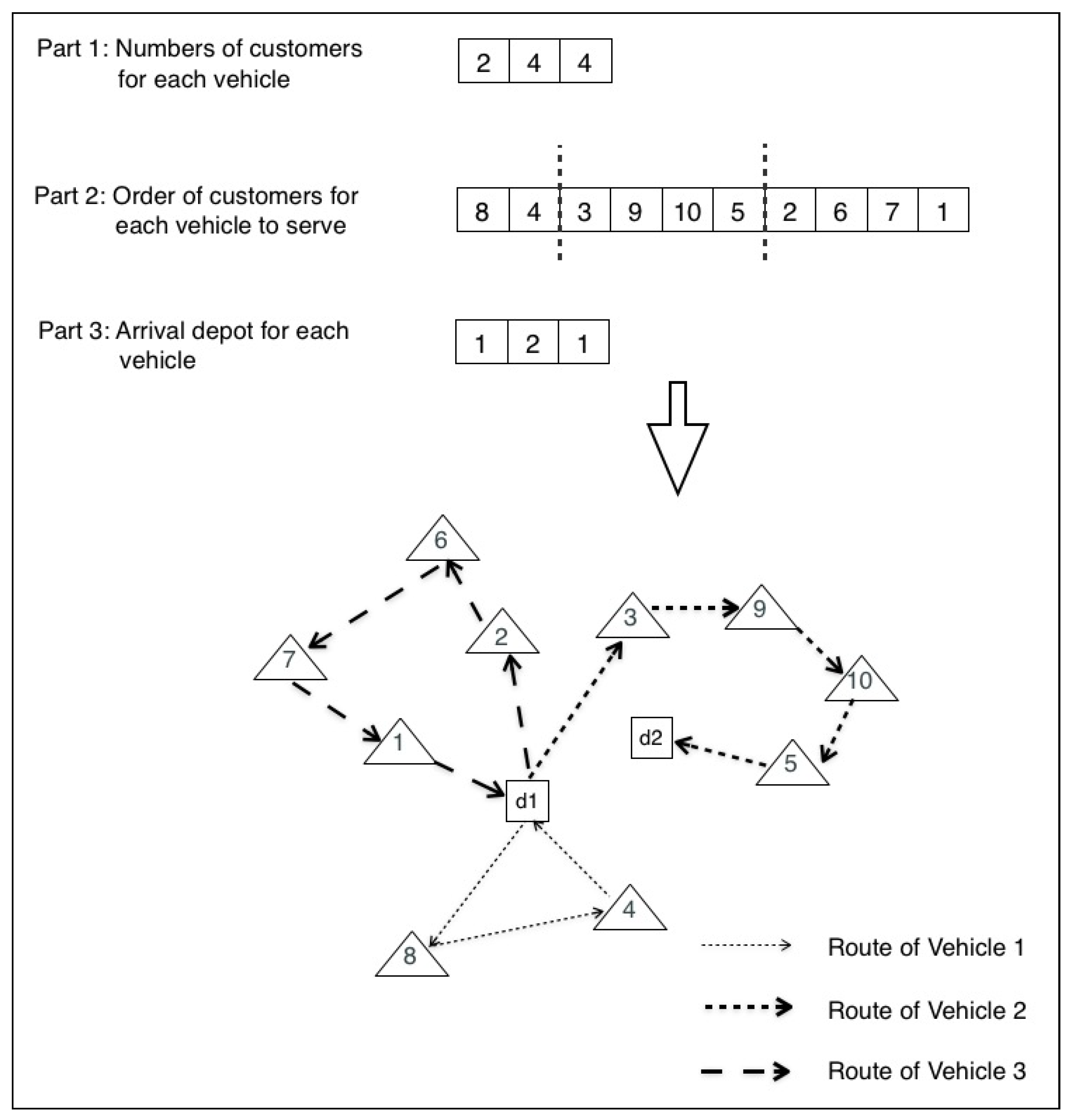
Solutions are represented by chromosomes. By analyzing the proposed problem, we find that the factors which can affect the objective values are: (1) assignment of each customer to exactly one vehicle; (2) the sequence of customers to be served by each vehicle; and (3) arrival depot of each vehicle. Therefore, in two heuristics, a solution is composed of three decision parts: (i) the first part is composed by the numbers of customers served by vehicles; (ii) the second part is the order of customers to be served by each vehicle; and (iii) the third part is the arrival depot of each vehicle.

Figure 1 illustrates the chromosome representation. Assume that there are 10 customers and 3 vehicles, and all vehicles depart from depot 1. The chromosome in Figure 1 shows that vehicle 1 serves 2 customers (8, 4) in order and arrives at depot 1, vehicle 2 serves 4 customers (3, 9, 10, 5) in order and then arrives at depot 2, and vehicle 3 serves 4 customers (2, 6, 7, 1) in order and arrives at depot 1.

4.3.2. Evaluation and Feasibility Check

The evaluation step is to determine fitness values of an individual. For our problem, evaluation procedure corresponds to the computation of total energy consumption and total tardiness of a solution. A chromosome must be translated into the routes of vehicles before evaluation.

Consider a chromosome S mentioned above. The route of each vehicle can be obtained accordingly as shown in Figure 1. If a vehicle serves no customer, the energy consumption and tardiness of this vehicle are set to be zero. Otherwise, let vector $pat{h}_k$ represents the route of vehicle k. For instance, $pat{h}_2=\{1,3,9,10,5,2\}$ denotes the route of vehicle 2 in Figure 1, where the first and the last element represent the departure depot and arrival depot of vehicle 2. The cumulative energy consumption $R_{ik}$ of vehicle k before it loads at a vertex $i\in N_0\cup N_1$ is detailed in constraints (10)–(17), and the tardiness $L_{ik}$ of vehicle k at a customer $i\in N_1$, is defined by constraints (18)–(23). The calculation of two fitness values, i.e., total energy consumption and total tardiness, are given by (1) and (2).

After a solution is generated, it is possible that this solution is infeasible, which violates some constraints provided by the formulation in Section 3. Feasibility check procedure is to ensure the feasibility of the problem. We can find that by using the solution representation in Section 4.3.1, constraints (3)–(8) and (24)–(25) are immediately satisfied, and constraints (10)–(23) correspond to the definition of cumulative energy consumption and tardiness. Therefore, the feasibility check procedure mainly focuses on checking whether the capacity constraint (9) is violated. If the feasibility check is not passed for a solution, that is, the load of at least one vehicle exceeds its capacity in the solution, then a very large penalty will be added to both of its fitness values in order to discard this solution through the non-dominated sorting procedure.

4.3.3. Population Initialization

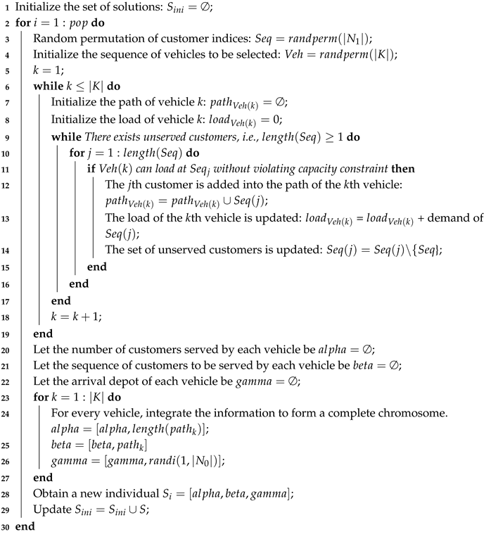
The initial population includes several feasible solutions. To generate an initial solution in $H_1$, firstly the indices of customers are sorted randomly, and based on that a vehicle is selected at random to serve customers one after another until its capacity limit is reached. Then for remaining unserved customers, another vehicle is chosen, and the same operation is repeated until each customer is served by exactly one vehicle. The arrival depot of each vehicle is randomly selected, after which the routes of all vehicles are determined and then coded by the solution representation method. The framework of population initialization in $H_1$ is illustrated in Algorithm 2.

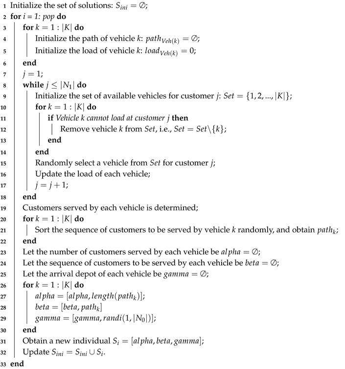
Population initialization in $H_2$ is shown in Algorithm 3. For each customer, there is an initial set of available vehicles, which can serve this customer without violating the capacity constraint. From every customer 1 to $|N_1|$, after the vehicle that serves each customer is randomly selected from the set of available vehicles, the load of this vehicle and the available vehicles for the next customer are updated. Then the sequence of customers served by each vehicle is randomly arranged, arrival depot of each vehicle is selected at random, and routes of all vehicles are determined and coded by solution representation method.

Algorithm 2:Population initialization in $H_1$.

Input: Problem parameters and population size $pop$

Algorithm 3:Population initialization in $H_2$.

Input: Problem parameters and population size $pop$

4.3.4. Selection

After the non-dominated sorting procedure is completed, initial solutions are sorted into different non-dominated ranks and their crowding distances are computed. It is implied that between two individuals with different ranks, the one with lower rank is preferred, when they are of the same front, the one with larger crowding distance is selected.

4.3.5. Genetic Operators

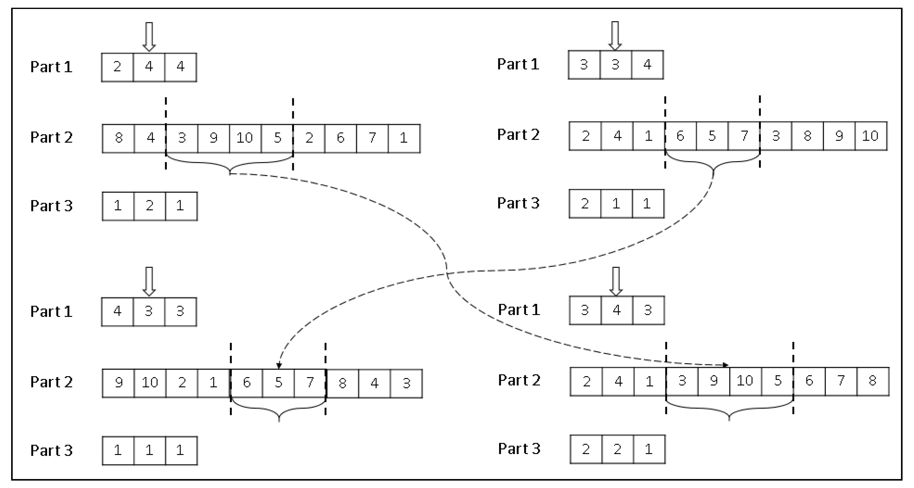
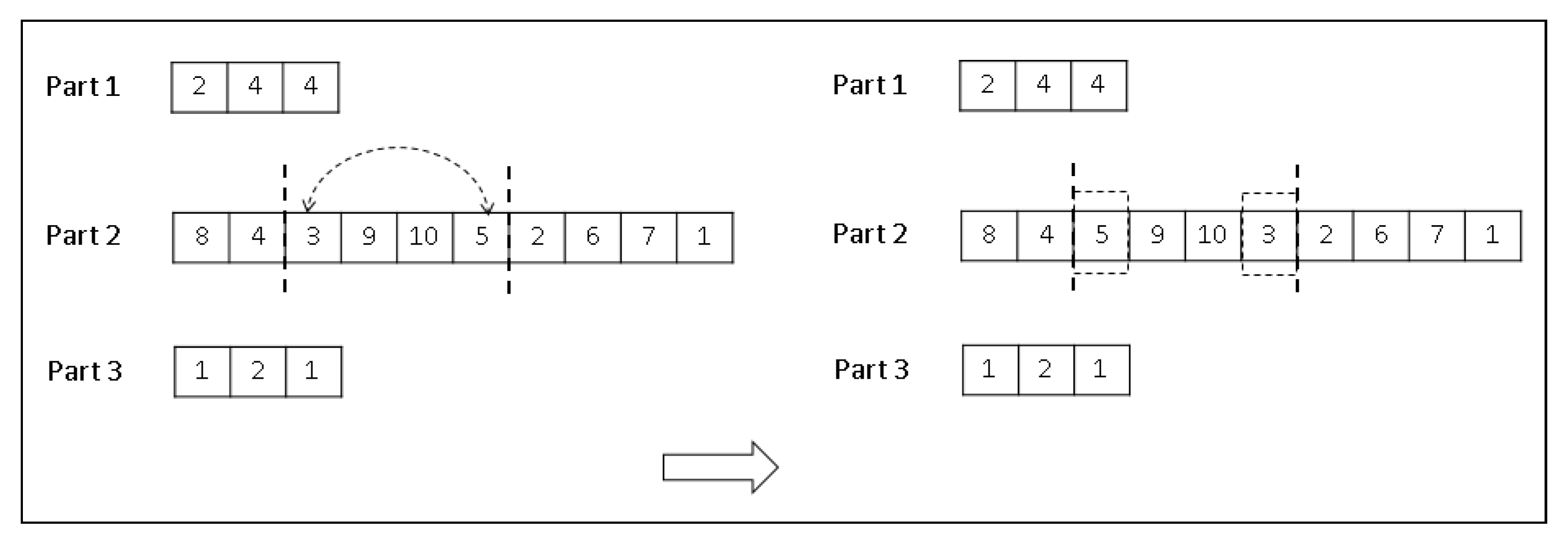
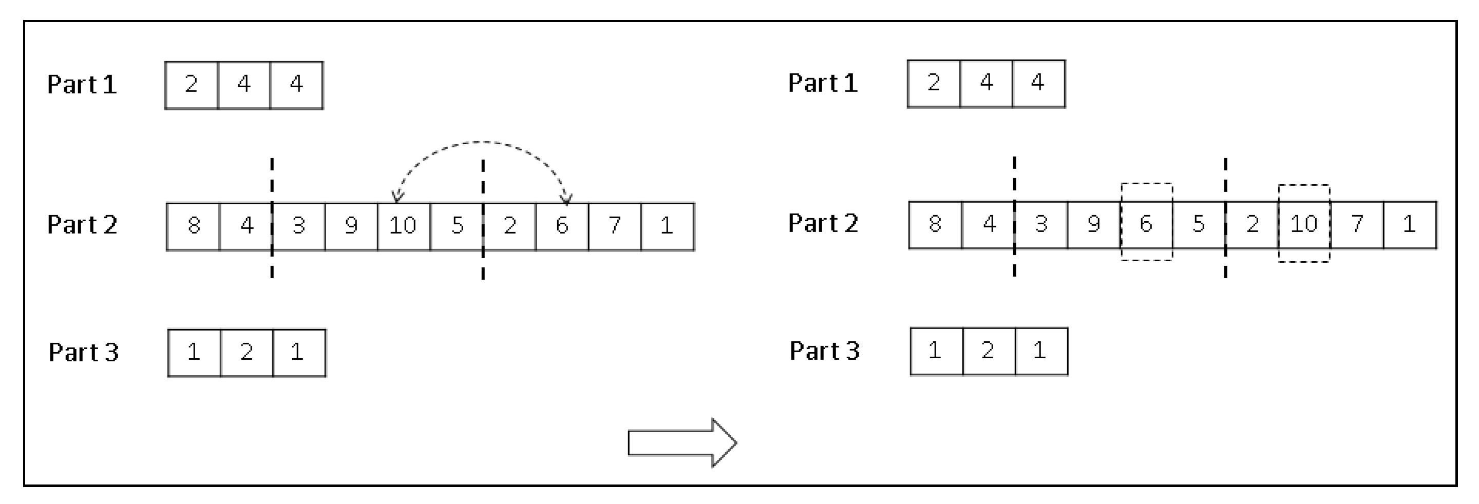
Genetic operators, including crossover and mutation procedure, are performed for reproducing offspring in each generation. The crossover procedure of $H_1$ is shown in Figure 2. We randomly choose a vehicle and exchange its routes between two parent solutions and assign remaining vehicles randomly for the unserved customers. For mutation procedure, there are two ways: (i) exchanging the sequences of two customers in the route of one certain vehicle, which is shown in Figure 3; and (ii) exchanging two customers served by different vehicles as shown in Figure 4.

In terms of crossover procedure in $H_2$, we focus on preserving similarities between two parental solutions. For each vehicle, if it serves the same customer in two parental solutions, then the customer will be still served by this vehicle in the offspring solutions. In addition, we randomly assign the remaining customers to vehicles, then arrange the sequence of customers to be served by each vehicle at random. There are two methods for mutation: (i) exchanging the sequences of two customers in the route of a certain vehicle as shown in Figure 3; and (ii) changing the terminal depots for vehicles by selecting a new depot randomly.

4.3.6. Recombination

During each iteration, the population which combines current solutions and offspring solutions will be updated. Population is sorted into various non-dominated ranks {F${}_1$, F${}_2$, …, F${}_t$, …} by non-dominated sorting procedure. Solutions in F${}_1$ are updated into the renewed population if the population size does not exceed $pop$. Then solutions in F${}_2$ are added into the renewed population as long as the population size is no more than $pop$, and so on. The operation will not be stopped until the population size exceeds $pop$ by adding the solutions in front F${}_t$. To maintain several $pop$ solutions, solutions in front F${}_t$ are selected by the selection procedure described in Section 4.3.4.

5. Computational Experiments

In this section, the performance of proposed methods is evaluated by 100 randomly generated instances, which includes small-, medium-, and large-size ones. All algorithms were coded in MATLAB R2014b. All computational experiments were conducted on a PC with 3.60 GHz processor and 8.00 GB RAM under windows 10 operating system. For the augmented $ϵ$-constraint method, CPLEX 12.6 is used to solve single-objective problems, computation time for each single-objective optimization and total computational time are limited within 7200 s and 36,000 s respectively.

For two NSGA-II-based heuristics, a preliminary analysis was conducted to fine-tune the parameters, which is presented in

Table 1. Parameters for heuristics.

Parameter	Value (${\mathit{H}}_1$)	Value (${\mathit{H}}_2$)
Population size ($pop$)	500	500
Generation number ($gen$)	20	20
Crossover probability	0.6	0.7
Mutation_1 probability	0.3	0.2
Mutation_2 probability	0.1	0.1

. Population size and generation number are set to be 500 and 20 respectively. In computational experiments, tournament size is set to be $0.5\times pop$ as in line with the classic NSGA-II in Deb et al. [56].

5.1. Data Generation

For small-size and medium-size instances, the data set is derived from instances for VRPTW proposed by Solomon [57]. Solomon’s benchmark problems have been grouped into three different types: C, R, and RC. Each type of data includes 8 to 12 instances with a central depot, 100 customers, homogeneous vehicles, and different time windows. Customers in type R are uniformly and randomly distributed, and those in type C have been clustered. Problems of RC-type are mixtures of both random and clustered locations. Time windows in sets of ’R1’, ’C1’ and ’RC1’ are narrow, while those in sets of ’R2’, ’C2’ and ’RC2’ are wider. Euclidean distances and traveling times are numerically identical.

We set the curb weight of each vehicle $w_k=\rho V_k$ with $\rho =0.15$ as in Kara et al. [43]. For instance, with $\left|N\right|$ customers, $\left|D\right|$ depots and $\left|K\right|$ vehicles, data set of customers are derived from the original benchmark problem R-101 (Solomon [57]) by considering the first $\left|N\right|$ customers. Euclidean coordinates of the depots are generated by considering the first $\left|D\right|$ depots detailed in

Table 2. Information of Depots and Vehicles in small- and medium- size problems.

Depote	$D_1$	$D_2$	$D_3$	$D_4$	$D_5$	$D_6$	$D_7$	$D_8$	$D_9$	$D_{10}$
X	27	35	29	40	20	22	30	40	38	42
Y	51	35	53	68	80	84	55	20	37	48
Vehicle	$T_1$	$T_2$	$T_3$	$T_4$	$T_5$	$T_6$	$T_7$	$T_8$	$T_9$	$T_{10}$
Capacity	200	150	130	170	120	250	280	190	270	240
Vehicle	$T_{11}$	$T_{12}$	$T_{13}$	$T_{14}$	$T_{15}$	$T_{16}$	$T_{17}$	$T_{18}$	$T_{19}$	$T_{20}$
Capacity	320	450	430	470	500	450	480	490	470	340
Vehicle	$T_{21}$	$T_{22}$	$T_{23}$	$T_{24}$	$T_{25}$	$T_{26}$	$T_{27}$	$T_{28}$	$T_{29}$	$T_{30}$
Capacity	420	450	430	570	500	450	380	410	370	340
Vehicle	$T_{31}$	$T_{32}$	$T_{33}$	$T_{34}$	$T_{35}$	$T_{36}$	$T_{37}$	$T_{38}$	$T_{39}$	$T_{40}$
Capacity	420	330	430	370	400	350	480	410	370	440
Vehicle	$T_{41}$	$T_{42}$	$T_{43}$	$T_{44}$	$T_{45}$	$T_{46}$	$T_{47}$	$T_{48}$	$T_{49}$	$T_{50}$
Capacity	420	430	530	470	400	450	480	510	570	540

, where the coordinates of the first 7 depots are in line with Dondo and Cerdá [28] and those of the last 3 depots are randomly generated. The capacities of vehicles are generated by considering the first $\left|K\right|$ vehicles in Table 2. Without loss of generality, departure depot for each vehicle is randomly assigned.

For large-size instances, data set is derived from Homberger’s instances of type S-R1-800. The generation of data is same as the method detailed above. Solomon’s instances and Homberger’s instances are available online at http://neo.lcc.uma.es/vrp/vrp-instances/capacitated-vrp-with-time-windows-instances/.

5.2. Performance Metrics

Since the output of a bi-objective optimization is a set of non-dominated solutions, solution quality is less straightforward. As stated in Liu et al. [58], an ideal bi-objective method has two features: (i) it can find a set of solutions close to the optimal Pareto front; and (ii) solutions have a large diversity. To evaluate the performance of the approaches, three widely used metrics, which are cardinality, hyper-volume ratio and average e-dominance, are introduced (Cheng et al. [59]).

Cardinality ($\mathcal{Q}$): this metric measures the number of non-dominated solutions obtained by each method (Van Veldhuizen and Lamont [60]). A larger $\mathcal{Q}$ implies a better solution set.

The hyper-volume Ratio ($\mathcal{H}$): This measure calculates the ratio of the hyper-volume ($HV$) of a solution set A and a reference set R, which is denoted as $H{V}_A$ and $H{V}_R$, separately. It is calculated as Equation (31):

$$\begin{array}{c}\hfill \mathcal{H}=H{V}_A/H{V}_R.\end{array}$$

(31)

The reference solution set can either be the exact Pareto front or a set of high quality non-dominated solutions. $HV$ implies the size of dominated space for a set of solutions (Zitzler et al. [61,62]). This indicator calculates the volume of a given region H. For bi-objective problems, $HV$ is equal to the union of the rectangle shaped by the nadir point and each point in the set of non-dominated solutions, the volume of overlapped area is only calculated once. A larger value of this metric implies a better set of solutions.

Average e-dominance ($\mathcal{D}$): this measure implies the average distance between a solution set A and the reference set R, which is shown in Equation (32). The closer the value of $\mathcal{D}$ to 1 implies a better performance.

$$\begin{array}{c}\hfill \mathcal{D}=\frac{1}{\left|R\right|}\sum _{x_R\in R}e(x,x_R),\end{array}$$

(32)

where,

$$\begin{array}{c}\hfill e(x,x_R)=\underset{x\in A}{min}max\left\{\frac{f_1(x)}{f_1(x_R)},\frac{f_2(x)}{f_2(x_R)}\right\}.\end{array}$$

5.3. Results and Discussion

Computational results obtained are reported in

Table 3. Computational results for small-size instances.

Set	($\left|\mathit{N}\right|,\left|\mathit{D}\right|,\left|\mathit{K}\right|$)	Augmented $\mathit{ϵ}$-Constraint Method		${\mathit{H}}_1$				${\mathit{H}}_2$
		$\mathcal{Q}$	CT	$\mathcal{Q}$	$\mathcal{H}$	$\mathcal{D}$	CT	$\mathcal{Q}$	$\mathcal{H}$	$\mathcal{D}$	CT
1	(5,1,1)	3	6.5	3	1.000	1.000	15.1	3	1.000	1.000	3.8
2	(5,1,2)	3	10.9	3	1.000	1.000	22.5	3	1.000	1.000	4.1
3	(5,1,3)	4	13.8	4	1.000	1.000	24.2	4	1.000	1.000	4.4
4	(5,1,4)	3	17.5	3	1.000	1.000	28.5	3	1.000	1.000	4.6
5	(5,2,2)	5	16.4	5	1.000	1.000	24.1	5	1.000	1.000	4.1
6	(5,2,3)	3	25.5	3	1.000	1.000	28.3	3	1.000	1.000	4.5
7	(5,2,4)	2	81.6	2	1.000	1.000	29.3	2	1.000	1.000	4.6
8	(6,1,1)	6	17.3	6	1.000	1.000	15.5	6	1.000	1.000	3.8
9	(6,1,2)	6	24.6	6	1.000	1.000	22.2	6	1.000	1.000	4.1
10	(6,1,3)	4	34.6	4	1.000	1.000	26.8	4	1.000	1.000	4.3
11	(6,1,4)	4	46.7	4	1.000	1.000	28.0	4	1.000	1.000	4.2
12	(6,2,2)	8	42.3	7	1.028	0.981	23.2	7	0.999	0.955	4.5
13	(6,2,3)	3	86.7	3	1.000	1.000	27.3	3	1.000	1.000	4.3
14	(6,2,4)	2	537.5	2	1.000	1.000	28.8	2	1.000	1.000	4.7
15	(7,1,1)	6	20.5	6	1.000	1.000	15.2	6	1.000	1.000	4.0
16	(7,1,2)	10	142.6	11	0.843	1.315	23.4	11	1.000	1.316	4.2
17	(7,1,3)	12	1336.1	7	0.903	1.110	26.6	8	0.954	1.109	4.5
18	(7,1,4)	8	491.9	7	0.734	1.546	26.7	7	0.774	1.001	4.7
19	(7,2,2)	15	162.4	11	0.821	1.107	27.8	15	0.999	1.158	4.3
20	(7,2,3)	6	420.6	5	0.728	1.028	23.6	5	0.729	1.039	4.5
21	(7,2,4)	5	6727.1	4	0.859	0.978	27.4	4	0.948	1.099	4.7
22	(8,1,1)	5	79.9	7	0.813	1.013	28.3	6	0.853	1.043	3.9
23	(8,1,2)	14	585.6	14	0.963	1.381	15.3	13	0.993	1.235	4.3
24	(8,1,3)	13	2095.6	12	0.929	1.135	23.4	14	0.920	1.130	4.6
25	(8,1,4)	13	15,447.1	11	0.929	1.212	26.9	8	0.757	1.052	4.8
26	(8,2,2)	18	11,497.6	8	0.612	1.318	27.8	17	0.980	1.291	4.3
27	(8,2,3)	8	12,326.1	9	0.353	2.997	24.1	13	1.014	1.240	4.6
28	(8,2,4)	10	16,209.9	3	0.714	1.006	27.0	5	0.731	1.006	4.8
29	(9,1,1)	6	804.3	8	0.998	1.212	15.7	4	1.000	1.011	3.9
30	(9,1,2)	12	8179.8	13	0.726	1.398	24.0	8	0.991	1.240	4.3
31	(9,1,3)	6	14,913.9	13	0.664	1.307	27.5	9	0.790	1.094	4.7
32	(9,1,4)	6	16,278.0	7	0.476	1.055	28.3	6	1.000	1.025	4.9
33	(9,2,2)	14	9962.1	9	1.244	1.388	24.5	16	0.824	1.175	4.4
34	(9,2,3)	4	31,429.1	8	0.606	1.263	27.4	3	0.616	1.067	4.7
35	(9,2,4)	6	36,000.0	2	0.737	1.003	28.4	7	0.778	1.069	4.9
36	(10,1,1)	12	7174.1	11	0.776	1.185	15.7	9	0.984	1.224	4.0
37	(10,1,2)	15	18,367.6	6	0.541	1.420	24.0	9	0.917	1.067	4.4
38	(10,1,3)	10	22,393.4	7	0.769	1.205	27.7	11	0.966	1.321	4.8
39	(10,1,4)	7	28,547.6	12	0.993	1.198	28.4	9	0.810	1.469	5.0
40	(10,2,2)	11	29,842.2	9	1.216	1.386	25.1	18	1.012	1.296	4.2
41	(10,2,3)	12	34,639.8	7	1.288	1.351	28.3	7	1.364	1.163	4.8
42	(10,2,4)	9	36,000.0	8	0.898	1.354	28.7	9	0.928	1.387	5.1
43	(11,1,1)	10	36,000.0	9	1.124	1.488	15.7	6	1.074	1.325	4.2
44	(11,1,2)	12	36,000.0	5	0.759	1.431	23.6	11	1.363	1.083	4.6
45	(11,2,2)	8	36,000.0	8	1.068	1.590	24.5	6	1.089	1.048	4.6
Average		7.978	10,467.7	6.956	0.891	1.208	24.551	7.444	0.959	1.103	4.438

,

Table 4. Computational results for medium-size instances.

Set	($\left|\mathit{N}\right|,\left|\mathit{D}\right|,\left|\mathit{K}\right|$)	Reference	${\mathit{H}}_1$				${\mathit{H}}_2$
		$\mathcal{Q}$	$\mathcal{Q}$	$\mathcal{H}$	$\mathcal{D}$	CT	$\mathcal{Q}$	$\mathcal{H}$	$\mathcal{D}$	CT
46	(20,2,3)	7	5	0.834	1.114	28.3	8	0.858	1.156	5.9
47	(20,3,4)	14	10	0.843	1.204	29.2	13	1.004	1.204	6.3
48	(25,2,3)	6	7	0.632	1.189	28.9	5	1.006	1.259	7.6
49	(25,3,4)	13	3	0.834	0.918	29.7	18	0.932	1.138	7.4
50	(30,2,3)	6	9	0.187	1.148	28.8	6	1.000	1.085	9.8
51	(30,3,4)	6	9	0.544	1.053	29.5	10	0.934	1.138	9.8
52	(35,2,5)	6	11	0.145	1.157	30.4	6	1.000	1.109	10.7
53	(35,3,6)	12	8	0.593	1.106	31.1	14	0.972	1.077	8.9
54	(40,2,5)	16	10	0.692	1.115	31.0	15	1.051	1.183	14.3
55	(40,3,6)	14	14	1.000	1.085	31.4	16	1.028	1.297	13.8
56	(45,2,5)	15	5	0.171	1.409	31.3	15	1.000	1.178	4.6
57	(45,3,6)	16	9	0.787	1.118	32.2	16	0.995	1.115	4.2
58	(50,2,7)	15	10	0.998	1.041	32.5	10	0.990	1.064	15.4
59	(50,3,8)	9	11	0.932	1.124	33.4	8	0.970	1.129	14.2
60	(55,2,7)	10	6	0.835	1.098	33.1	9	0.948	1.024	17.5
61	(55,3,8)	6	9	0.538	1.076	33.2	6	1.000	1.061	16.2
62	(60,2,7)	11	5	0.907	0.978	33.2	18	0.861	1.071	21.3
63	(60,3,8)	15	20	0.648	1.095	33.2	14	0.999	1.117	19.1
64	(65,3,9)	11	9	0.837	1.002	34.5	11	1.000	1.111	20.0
65	(65,4,10)	3	3	0.786	1.175	34.6	3	1.000	1.085	17.5
66	(70,3,9)	5	5	0.651	1.174	35.0	5	1.000	1.023	24.9
67	(70,4,10)	6	9	0.498	1.016	35.5	6	1.000	1.059	21.2
68	(75,3,9)	15	4	0.861	1.024	34.6	16	0.898	1.083	28.7
69	(75,4,10)	14	7	0.969	0.998	35.6	20	0.811	1.062	24.9
70	(80,3,11)	15	12	0.855	1.025	38.1	15	0.928	1.082	25.1
71	(80,4,12)	11	7	0.734	1.013	35.7	11	0.923	1.059	22.4
72	(85,3,11)	9	26	0.628	1.113	35.7	9	1.000	1.115	31.2
73	(85,4,12)	13	11	0.867	1.099	36.6	6	1.252	1.062	29.2
74	(90,4,11)	19	14	0.955	1.076	36.5	13	0.974	1.066	27.2
75	(90,5,12)	8	7	0.626	1.043	36.6	9	0.981	1.045	32.9
76	(95,5,13)	17	12	0.900	1.048	38.1	12	0.986	1.024	32.8
77	(95,6,14)	10	12	0.639	1.062	31.2	9	1.000	1.053	30.4
78	(100,5,13)	14	9	0.752	1.050	38.1	13	0.937	1.043	32.6
79	(100,6,14)	12	11	0.819	1.164	37.8	12	0.976	1.055	32.7
Average		11.147	9.382	0.721	1.092	33.421	11.088	0.977	1.101	19.412

and

Table 5. Computational results for large-size instances

Set	($\left|\mathit{N}\right|,\left|\mathit{D}\right|,\left|\mathit{K}\right|$)	Reference	${\mathit{H}}_1$				${\mathit{H}}_2$
		$\mathcal{Q}$	$\mathcal{Q}$	$\mathcal{H}$	$\mathcal{D}$	CT	$\mathcal{Q}$	$\mathcal{H}$	$\mathcal{D}$	CT
80	(200,5,20)	9	7	0.879	1.048	47.9	9	0.762	1.089	182.2
81	(200,6,22)	16	16	1.000	1.059	48.2	14	0.789	1.047	170.9
82	(250,5,22)	12	14	0.713	1.050	54.4	13	0.920	1.056	312.0
83	(250,6,25)	15	10	0.863	0.998	54.2	15	0.976	1.023	238.5
84	(300,6,25)	12	10	0.874	1.025	60.1	11	0.898	1.011	353.9
85	(300,7,27)	14	14	0.970	1.024	62.1	10	0.781	1.042	338.7
86	(350,7,27)	13	7	0.854	1.022	67.4	7	0.743	1.032	572.8
87	(350,8,30)	6	3	0.475	1.027	68.7	8	0.534	1.014	424.8
88	(400,8,30)	11	10	0.999	1.011	74.8	6	1.002	1.010	631.1
89	(400,9,32)	11	10	0.645	1.017	74.1	6	0.816	1.008	543.1
90	(450,9,34)	18	4	0.664	1.238	83.1	18	0.987	1.017	487.9
91	(450,10,35)	16	10	0.751	1.210	83.7	16	0.962	1.023	478.7
92	(500,10,36)	16	16	0.546	1.033	91.7	5	0.712	1.028	922.9
93	(500,8,37)	10	10	1.044	1.045	92.4	7	1.012	1.008	883.8
94	(550,9,39)	9	5	0.750	1.243	102.7	13	0.824	1.098	777.5
95	(550,10,40)	8	7	0.865	1.147	101.7	12	0.820	1.067	1012.0
96	(600,9,42)	10	10	1.000	1.013	111.2	9	0.516	1.039	1188.0
97	(650,9,43)	15	11	0.979	1.011	119.4	12	0.594	1.012	1337.9
98	(700,9,45)	11	11	0.986	1.013	131.0	13	0.592	1.034	1710.1
99	(750,9,47)	4	8	0.852	1.005	130.6	8	0.634	1.046	1953.4
100	(800,10,50)	8	8	1.000	1.004	153.2	15	0.463	1.045	2080.3
Average		11.619	9.571	0.843	1.059	86.314	10.809	0.778	1.045	790.500

. For each instance, we run each algorithm 30 times independently and obtain the average value of these results (Cheng et al. [59]).

Table 3 represents the computational results of the small-size instances in which the number of customers ranges from 5 to 11. Since augmented $ϵ$-constraint method direct uses CPLEX and it can obtain the optimal Pareto fronts, which is selected as the reference set. It is understandable that both $\mathcal{H}$ and $\mathcal{D}$ value of the reference set itself are equal to 1, therefore the values of these two indicators of augmented $ϵ$-constraint method are omitted in Table 3. By comparing the value of $\mathcal{Q}$ of the methods, it can be seen that on average the performance of $H_1$ is a bit worse in terms of the number of non-dominated solutions. Meanwhile, it also can be seen that the average value of $\mathcal{H}$ of $H_2$ is larger and closer to 1 compared with that of $H_1$, which implies that the solutions yielded by $H_2$ have similar quality to the exact Pareto font in terms of dominated space on average. Besides, according to the computational results, we can find that the average $\mathcal{D}$ value of $H_2$ is closer to 1, indicating that the average distance from solutions of $H_2$ to the reference set is smaller than that of $H_1$. Moreover, $H_2$ performs better in terms of computational time. For small-size instances, concluding, $H_2$ is much more efficient than $H_1$.

In the meantime, CPLEX loses its power to solve the problem exactly as it scales up, even failing to obtain optimal solutions for instances with more than 12 customers. Then, for the medium-size and large-size instances, the reference solution set is formed by selecting the non-dominated solutions from the combination of the two fronts obtained by the heuristics. Both algorithms can obtain approximate solutions for instances with 20 to 100 customers within 40 s.

Table 4 presents the computational results of the medium-size instances. The average computational time of $H_1$ is about 1.72 times that of $H_2$, which shows that $H_2$ performs better in terms of the computational time. Furthermore, it can be seen that the average number of non-dominated solutions yielded by $H_1$ is slightly less than that obtained by $H_2$. By comparing $\mathcal{H}$ values of two heuristics, we can find that the solutions yielded by $H_2$ have higher quality than $H_1$ on average. Besides, there is little difference between the average $\mathcal{D}$ values of two heuristics, which implies that the distance between the solutions obtained by the heuristics is small. For medium-size instances, to conclude, $H_2$ performs better than $H_1$ in terms of computation time, the number of non-dominated solutions. and the solution quality.

Computational results of large-size instances with 200 to 800 customers are reported in Table 5. It can be obtained that the computational time of $H_2$ increases much faster than $H_1$ as the problem scales up, which implies that $H_1$ is relatively stable and performs better for large-size instances in terms of computational time. The quality of solutions obtained by $H_1$ is higher than that of $H_2$ in terms of the average value of $\mathcal{H}$. However, the average number of solutions obtained by $H_1$ is less than that yielded by $H_2$. Moreover, we can find that the average $\mathcal{D}$ value of solutions of $H_1$ is slightly larger than that of $H_2$.

By comparing the results of two methods under different sizes of problems, we can find that, on average: (1) two heuristics are much more efficient than the augmented $ϵ$-constraint method incorporating with CPLEX in terms of computational time; (2) for small-size and medium-size instances, $H_2$ performs better than $H_1$ in terms of solution quality and computational time; (3) for large-size instances, $H_1$ outperforms $H_2$ in terms of computational time and the solution quality; and (4) for large-size instances, $H_2$ can help obtain more non-dominated solutions than $H_1$.

6. Conclusions

This paper investigated a bi-objective VRP with soft time windows and multiple depots, which aims to minimize total energy consumption and customer dissatisfaction simultaneously. A bi-objective mixed-integer linear programming model is presented for the problem. Then augmented $ϵ$-constraint method are adopted to obtain the exact optimal Pareto front for small-size problems, and two NSGA-II-based heuristics are designed to obtain approximate Pareto solutions for medium- and large-size problems. Computational experiments are conducted. The results show that $H_2$ performs relatively better than $H_1$ for small- and medium-size problems. For large-size problems, $H_2$ could find more Pareto solutions, while $H_1$ is able to obtain approximate Pareto fronts with better convergence in less computation time.

In addition, the property of the investigated problem is not fully explored, which may be the main limitation of this study.

For future research, several interesting issues may be addressed. Firstly, some other factors that may affect the objectives may be considered, such as the traffic conditions and the acceleration of vehicles. Besides, we may extend the study to other variants of the investigated problem, e.g., periodic VRP and pickup and delivery problems. Moreover, we also can combine the proposed method with other heuristics to develop more efficient solutions.